Evaluation of the Influence of Field Conditions on Aerial Multispectral Images and Vegetation Indices

Abstract

Remote sensing is a method used for monitoring and measuring agricultural crop fields. Unmanned aerial vehicles (UAV) are used to effectively monitor crops via different camera technologies. Even though aerial imaging can be considered a rather straightforward process, more focus should be given to data quality and processing. This research focuses on evaluating the influences of field conditions on raw data quality and commonly used vegetation indices. The aerial images were taken with a custom-built UAV by using a multispectral camera at four different times of the day and during multiple times of the season. Measurements were carried out in the summer seasons of 2019 and 2020. The imaging data were processed with different software to calculate vegetation indices for 10 reference areas inside the fields. The results clearly show that NDVI (normalized difference vegetation index) was the least affected vegetation index by the field conditions. The coefficient of variation (CV) was determined to evaluate the variations in vegetation index values within a day. Vegetation index TVI (transformed vegetation index) and NDVI had coefficient of variation values under 5%, whereas with GNDVI (green normalized difference vegetation index), the value was under 10%. Overall, the vegetation indices that include near-infrared (NIR) bands are less affected by field condition changes.

1. Introduction

In recent years, many studies have illustrated how unmanned aerial vehicles (UAVs) or drones can be used in crop monitoring and remote sensing in agriculture [1]. During the last decade, camera-equipped drones have evolved to become effective tools for crop and agroecosystem monitoring. Typically, agricultural drones are designed to carry different types of cameras [2]. Depending on the measurements, different camera technologies are being used, including RGB, multispectral, hyperspectral, and thermal cameras. There are obvious differences between the camera technologies, especially regarding image resolution and costs. Multiple cameras or other sensors, such as LiDAR, can be used for simultaneous monitoring for more extensive data sets [3,4]. A typical application of UAVs involves measuring crop diseases, the phenotypic traits of plants, such as crop height [5], and mildew in a vine field [6].

Another application for agricultural drones involves crop yield prediction, which can be conducted by calculating a vegetation index or multiple vegetation indices [7]. Qi et al. [8] estimated peanut (Arachis hypogaea) chlorophyll content by multispectral drone photography and calculated eight vegetation indices. They used machine learning (namely neural networks) for chlorophyll content estimation. Machine learning is increasingly being used for processing UAV image data [9] and recognizing plants from image data, such as weeds, and in invasive plant detection [10]. Satellites are actively being used for crop monitoring and their imaging data can be useful in agricultural crop production. The image resolutions of satellite data are typically lower than in drone imaging; satellite availability and coverage are still limited.

In general, most of the research studies focus on analyzing the correlation between imaging data and crop properties. Regarding aerial imaging in agricultural crop production, there seems to be two areas under special interest: (1) biomass or crop yield prediction by using vegetation indices and (2) weed or plant detection. In many studies, the vegetation index is the main property calculated for the crop. There is also growing interest in monitoring phenotypic traits by UAVs (but then the vegetation index is not necessarily a useful property). At times, plant-specific indices are derived from conventionally used vegetation indices to better describe plant-growing dynamics; for instance, Cao et al. [11] developed a wide-dynamic-range vegetation index for sugar beets. As the UAV studies are typically conducted with hyperspectral or multispectral cameras, the reflectance conditions may have an importance influence on the results. There have been studies on how the atmosphere affects the spectral bands on multi/hyperspectral images taken with satellites and drones. One hypothesis of this study is that different field and weather conditions influence the images taken by multispectral cameras and, therefore, the vegetation index values.

Vegetation indices are created by combining reflectance values from multiple spectral bands. Vegetation indices are used to minimize disturbances that can be caused by external factors [12,13,14]. For example, small aerosols in the atmosphere can cause disturbances in the multispectral images by absorbing and refracting the radiation coming from the sun. However, the atmospheric effects on drone images are very small when flying under 100 m [15]. Vegetation indices are typically used to evaluate different crop properties, such as biomass or nitrogen content [14,16,17]. There have also been studies where vegetation chlorophyll content have been estimated by using different vegetation indices [18]. One of the most used vegetation indices is NDVI (normalized difference vegetation index) [19]. NDVI has been studied as a health indicator of vegetation; it can also be used in estimating crop density because vegetation and bare soil have different NDVI values [20,21]. SARVI (soil adjusted and atmospherically resistant vegetation index) is an example of a vegetation index that mitigates the disturbances that are caused by the atmosphere and soil [12,13].

Vegetation indices can be used separately to evaluate crop properties, but in most research studies, more accurate crop models have been built by simultaneously using multiple indices and spectral bands. Multilinear regression and neural networks are especially used in combining the data from multiple vegetation indices for creating a model that can estimate different crop properties [16,22,23,24].

Because vegetation indices are widely used to describe crop properties in research evaluations, it is important to understand the influences of field conditions on the measurements. There have only been a few studies where multiple vegetation indices were compared, focusing on how they were affected by the different weather conditions during the growing season. In particular, the northern conditions can present challenges due to low solar elevation angles and changing weather conditions. The objective of this study was to measure and analyze how different field and weather conditions affect the multispectral camera’s reflectance and vegetation index values in northern latitudes. Aerial imaging measurements were done in multiple fields, different times of the day, different stages of the growing season, and in two different years. The measured imaging data were processed for identifying the underlying factors influencing the spectral data. Index values were calculated for 15 different vegetation indices. The results were analyzed to understand the lighting and in-field condition influences on the reflectance values. The results from this study will help researchers understand how different field and weather conditions affect the multispectral images and vegetation indices. These types of results will increase the overall understanding of the usability of different vegetation indices regarding the field conditions. They will also help researchers plan future UAV measurements so that the multispectral images can be taken at optimal conditions.

2. Materials and Methods

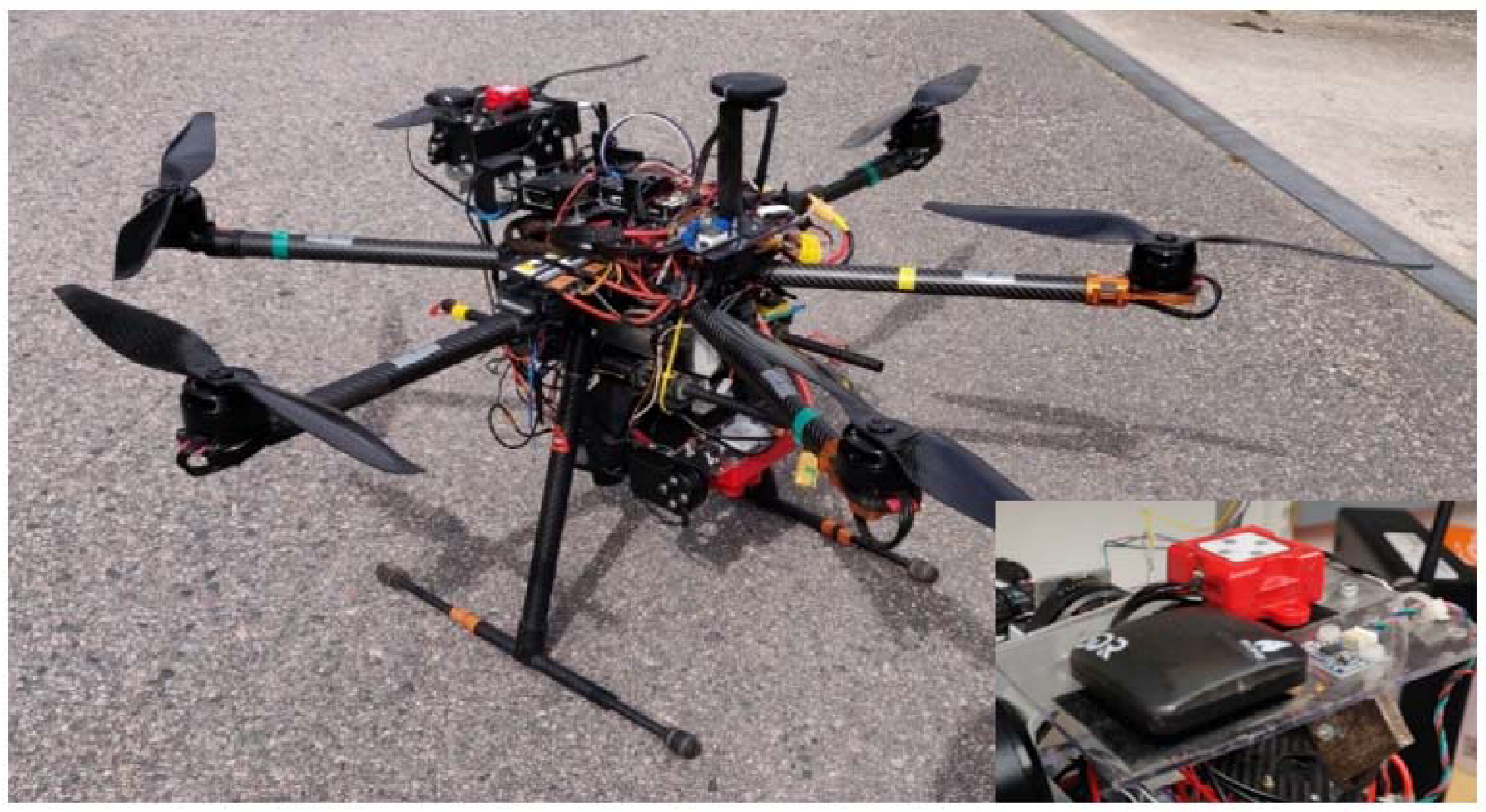
2.1. Custom-Built Unmanned Aerial Vehicle (UAV)

A custom-built hexacopter was developed for the research. The UAV is presented in Figure 1. The drone frame is a Tarot T960 that has a diameter of approximately one meter. The drone has six brushless motors (T-Motor U7 2.0 420 KV) with 18-inch (45.7 cm) propellers (Tarot 1855). Each motor has its own electronic speed controller (ESC) (T-motor T80A). The flight controller is a Pixhawk 2 cube. The whole drone was powered by one 14,000 mAh LiPo battery with six cells in series, resulting in nominal voltage of 22.2 V. The drone weight is 10 ± 0.5 kg (including battery weight, cameras, and their gimbals); the estimated flight time was 7 min, which left approximately a 30% charge in the battery after a flight mission. This was done to ensure a longer lifespan of the batteries and to prevent voltage drops during the flights.

Automatic flight missions were used to take images from the crops. These flight missions were planned with the Mission Planner software. The flights were planned to have a side-overlap of 80% for good coverage of the crop. The camera manufacturer recommends an overlap of over 75% for good results. A multispectral camera was triggered to take pictures in one second intervals. The target speed for the drone was 6 m/s and the flight altitude was set to 50 m, which resulted in 43.5 m × 32.6 m footprints in multispectral images.

2.2. Multispectral Camera

The images were taken with a Micasense Rededge 3 multispectral camera. It can take images from five different spectral bands (green (560 nm), blue (475 nm), red (668 nm), Rededge (717 nm), and near-infrared (NIR, 840 nm)). The multispectral camera had its own gimbal, which made imaging processing more robust. The camera’s light sensor was attached to a separate gimbal, as seen in Figure 1, which reduced the error caused by the sensor tilting away from the sun, which can create a shadow on the sensor.

Calibration images were taken before every flight according to the camera manufacturer’s own reflectance panel. This panel had specific reflectance values for each spectral band that could be used in Pix4D software to calibrate drone images.

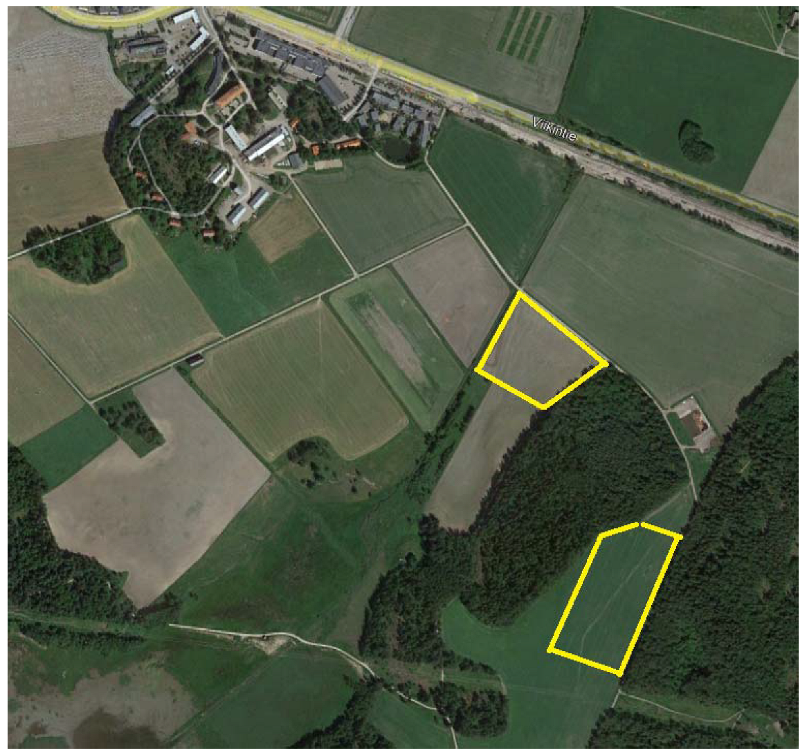
2.3. Research Fields

Research fields were located at the Viikki Research Farm, the University of Helsinki (Figure 2). In 2019 and 2020, images were taken in the Mölylä field (located at 60°13’08.4”N and 25°01’39.6”E) and Koirasuo field (located at 60°12’56.2”N and 25°01’50.2”E), respectively. Soil samples were taken on 21 October 2019 from both fields for cultivation purposes. Both fields had the same soil types (silt clay loam and fine sandy till). Koirasuo had higher organic matter content (6–20%) compared to Mölylä (3–12%). The pH values were very similar on both fields (Koirasuo 5.6–5.9 and Mölylä 5.7–6).

On the fields, there were 10 fixed locations approximately 8 m² in size from which the vegetation index values were calculated. Figure 3 illustrates the image data acquired from the measurement points on the fields. The fields were sown on 28 April 2019 (Mölylä) and 7 May 2020 (Koirasuo). The crop fields were harvested on 21 August 2019 and 28 September 2020, respectively.

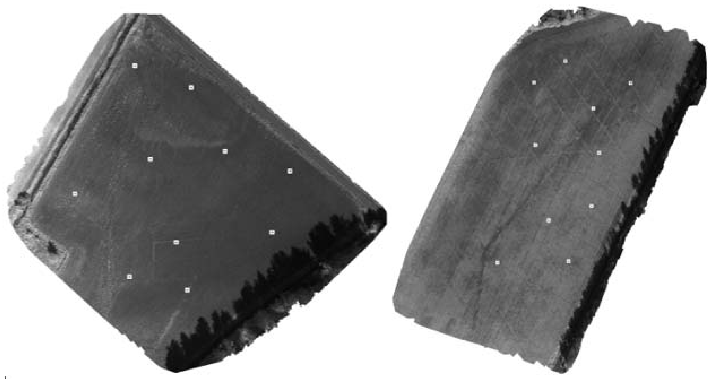
2.4. Field Measurements

This article presents the results from measurements made of a spring barley (Hordeum vulgare L.) field in 2019 and 2020. Drone images were taken on five different days as presented in

Table 1. Zadoks value for barley during the research time.

Date	17.7.2019	31.7.2019	28.6.2020	15.7.2020	1.8.2020
Zadoks value	83	87	69	83	86

. Images were taken at 8:00, 12:00, 16:00, and 20:00 (accurate flight times are presented in Appendix A,

Table A1. The accurate flight times for each measurement flight made in 2019 and 2020.

Flight Day	1. Flight	2. Flight	3. Flight	4. Flight
17.7.2019	8:00–8:15	11:45–12:00	15:51–16:06	19:40–19:55
31.7.2019	7:50–8:05	11:56–12:11	15:35–15:50	19:31–19:46
28.6.2020	8:06–8:31	12:12–12:34	15:56–16:17	19:47–20:10
15.7.2020	7:45–8:05	11:52–12:14	15:45–16:06	19:33–19:53
1.8.2020	7:45–8:08	11:57–12:17	15:36–15:57	19:22–19:42

). The field measured in 2019 was located in an open place so there were no large shadows on the field. During the 2020 measurements, the location changed, and the drone images were taken on a field that was located between two forests (Figure 2). These forests caused shadows on the field and on some of the measurement points. Due to the technical difficulties with the drone and the weather conditions, only two measurement days were made in 2019 and three days in 2020. Table 1 presents the Zadoks value of barley [25] for days when the drone images were taken.

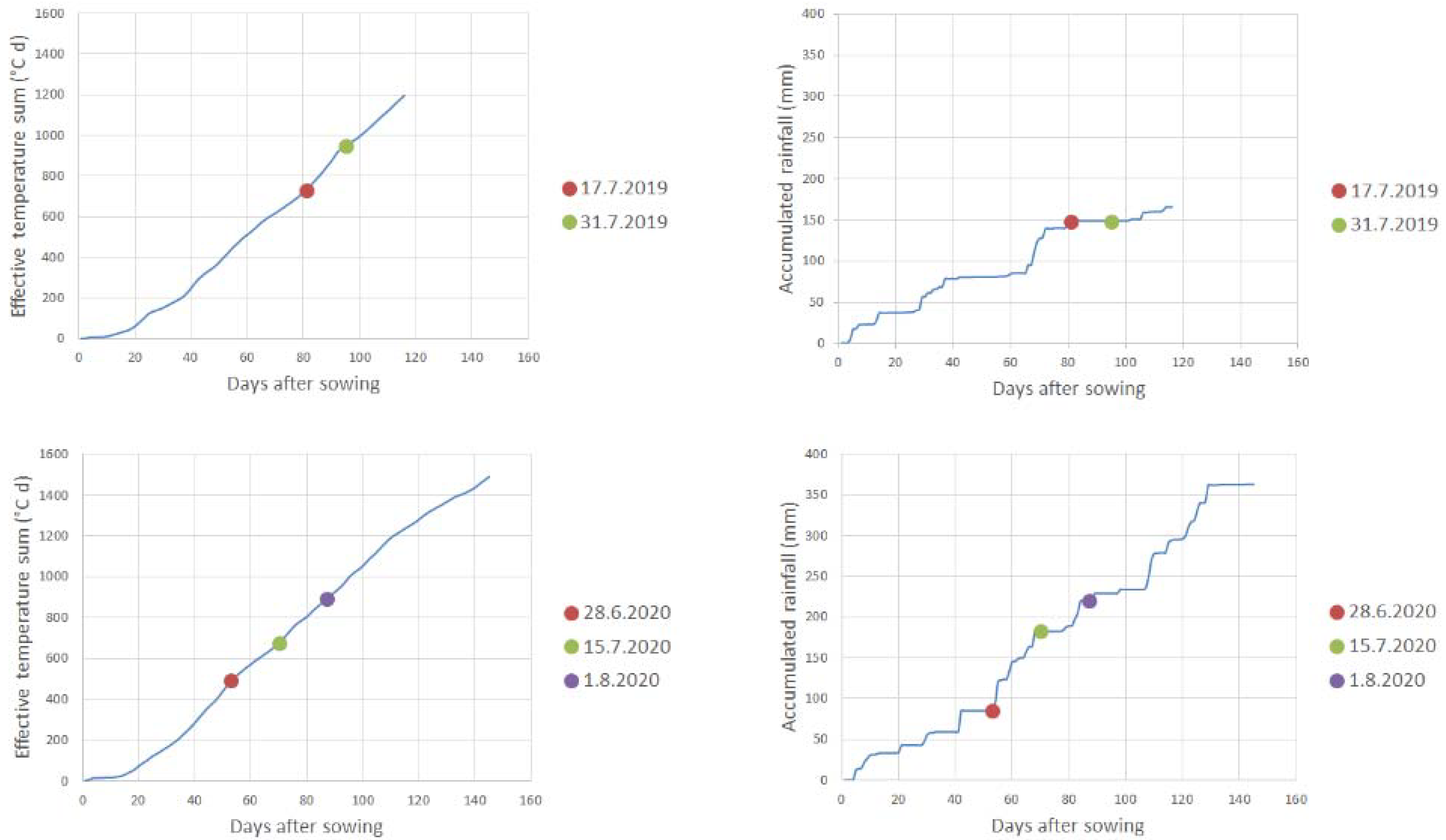
2.5. Weather Condition Measurements and Data

During the drone flights, the solar radiation was measured with total radiation PYR and photosynthetically active radiation (PAR) sensors. The PYR sensor (pyranometer) was LP02 and it measured radiation between 285 and 3000 nm. The PAR sensor was Apogee QSO-S, which measured radiation at wavelengths of 400–700 nm. A Campbell Scientific CR1000 datalogger was used to log the radiation values from the PYR and PAR sensors. The datalogger saved radiation values every 10 s. The radiation measurements started a few minutes before the drone started the flight and ended a few minutes after the drone landed.

The precipitation and air temperature data were measured at Kumpula, the Helsinki weather station, and can be freely downloaded from the Finnish Meteorological Institute’s website [26]. These weather measurement data were used to calculate the accumulated rainfall and effective temperature sum (above 5 °C) for the growing season (Figure 4).

2.6. Vegetation Indices

A total of 15 different vegetation indices were calculated from the 5 different spectral bands of the multispectral data.

Table 2. Vegetation indices and their equations that were used in this study. M-MTCI index was modified from the original MTCI index to fit the spectral bands of the used camera. The wavelengths for the five spectral bands: green (560 nm), blue (475 nm), red (668 nm), Rededge (717 nm), and near-infrared (NIR, 840 nm).

Index	Name	Equation	Source
DVI	Differenced vegetation index	$\mathrm{NIR}-\mathrm{RED}$	[27]
ExG	Excess green index	$2\times \mathrm{Green}-\mathrm{Red}-\mathrm{Blue}$	[28]
GEMI	Global environment monitoring index	$\eta \left(1-0.25\eta \right)-\frac{\mathrm{Red}-0.125}{1-\mathrm{Red}}$ where $\eta =\frac{(2\left({\mathrm{NIR}}^2-{\mathrm{Red}}^2\right)+1.5\mathrm{NIR}+0.5\mathrm{Red}}{\left(\mathrm{NIR}+\mathrm{Red}+0.5\right)}$	[29]
GNDVI	Green normalized difference vegetation index	$\frac{\mathrm{NIR}-\mathrm{Green}}{\mathrm{NIR}+\mathrm{Green}}$	[30]
GRVI	Green–red vegetation index	$\frac{\mathrm{Green}-\mathrm{Red}}{\mathrm{Green}+\mathrm{Red}}$	[31]
M-MTCI	Modified MERIS terrestrial chlorophyll index	$\frac{\mathrm{NIR}-\mathrm{Rededge}}{\mathrm{Rededge}-\mathrm{Red}}$	[32]
MSAVI2	Modified soil adjusted vegetation index	$\frac{2\times \mathrm{NIR}+1-\sqrt{{\left(2\times \mathrm{NIR}+1\right)}^2-8\left(\mathrm{NIR}-\mathrm{Red}\right)}}{2}$	[33]
NDRE	Normalized difference red edge index	$\frac{\mathrm{NIR}-\mathrm{Rededge}}{\mathrm{NIR}+\mathrm{Rededge}}$	[14]
NDVI	Normalized difference vegetation index	$\frac{\mathrm{NIR}-\mathrm{Red}}{\mathrm{NIR}+\mathrm{Red}}$	[19]
OSAVI	Optimized soil adjusted vegetation index	$1.16\ast \frac{\mathrm{NIR}-\mathrm{Red}}{\mathrm{NIR}+\mathrm{Red}+0.16}$	[34]
RGBVI	Red–green blue vegetation index	$\frac{{\mathrm{Green}}^2-\left(\mathrm{Blue}\ast \mathrm{Red}\right)}{{\mathrm{Green}}^2+\left(\mathrm{Blue}\ast \mathrm{Red}\right)}$	[35]
RI	Redness index	$\frac{\mathrm{Red}-\mathrm{Green}}{\mathrm{Red}+\mathrm{Green}}$	[36]
RVI	Ratio vegetation index	$\frac{\mathrm{Red}}{\mathrm{NIR}}$	[37]
TVI	Transformed vegetation index	$\sqrt{\mathrm{NDVI}+0.5}$	[38]
VIN	Vegetation index number	$\frac{\mathrm{NIR}}{\mathrm{Red}}$	[37]

presents the list of the vegetation indices with a description, calculation equation, and corresponding literature reference. One of the vegetation indices was modified from the original equation to suit the spectral bands of the multispectral camera (MTCI index). These modifications are presented in Table 2.

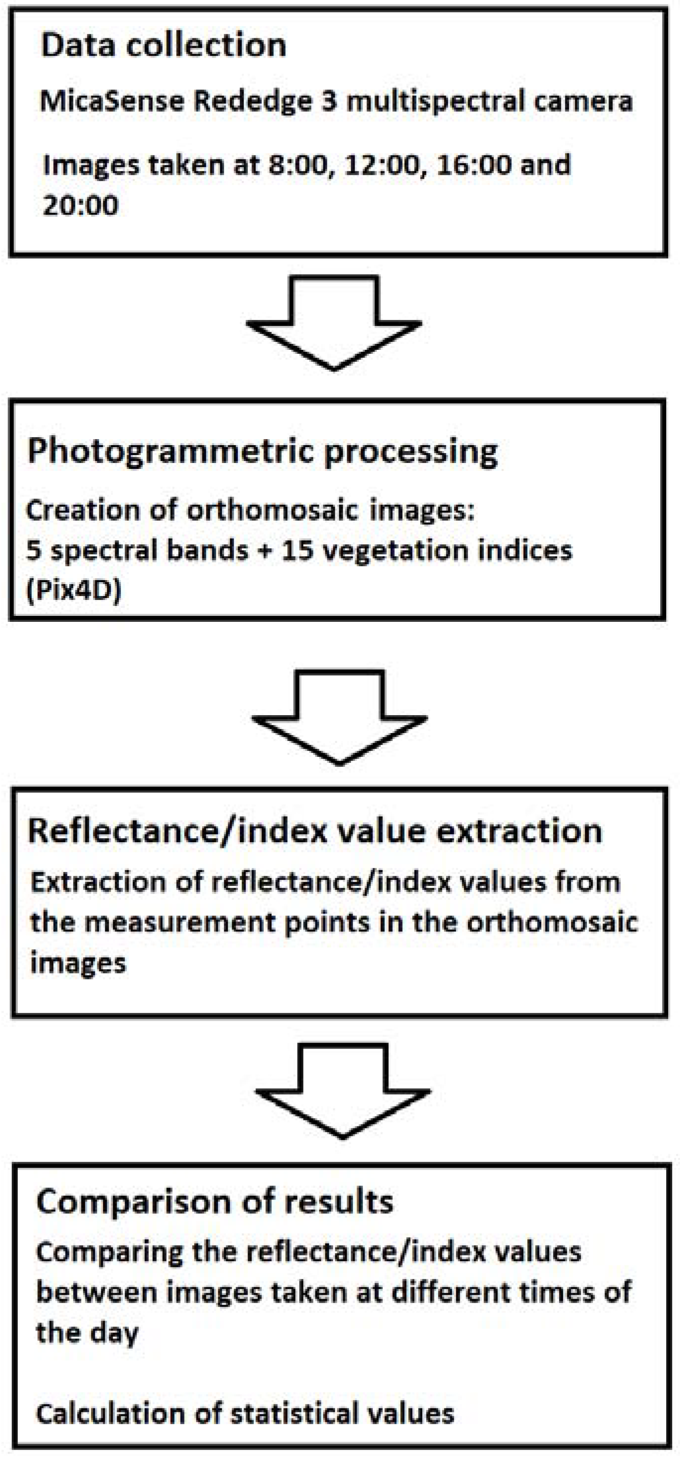
2.7. Image Data Processing

Multispectral images were processed with Pix4D software. This software created orthomosaic maps from each spectral band and vegetation index for the whole field area. When processing the multispectral images, the Ag multispectral template (which generates reflectance, index, classification, and application maps) was used on Pix4D. A DSM (digital surface model) was created using the inverse-distance weighting method. The software also used noise filtering and the surface smoothing setting was set to sharp when creating the DSM. From this DSM, a reflectance map was created for each spectral band. The software used values from the image metadata and the images from the calibration panel to correct the pixel values for the reflectance maps.

The resolutions of these orthomosaic maps were 3.4 cm/pixel. The 10 measurement points were identified from the orthomosaic maps with the help of ground control points (GCP) that were placed around the field. The coordinates of each measurement point were saved for later data processing. There was five GCP around the fields, which were also used to synchronize coordinates with other maps. All the orthomosaic images were processed with MATLAB software. The MATLAB code was used to calculate the reflectance and VI index values of an area of 8 m² for each measurement point. The whole data processing procedure is presented in Figure 5.

For the 28 June 2020 measurements, one measurement point was left out because erroneous data were observed in the multispectral images taking over an area of the field. The NIR reflectance values were 1.9 for this specific measurement point. All calculations for this one day (28 June 2020) were made from nine measurement points while the other days had ten measurement points.

To compare the variations between vegetation indices, the standard deviation (SD) (1) and coefficient of variation (CV) (2) values were calculated with the following equations:

$$SD=\sqrt{\frac{\sum \left|x-\overline{x}\right|}{n}}$$

(1)

$$\mathrm{CV}=\frac{SD}{\overline{x}\left(Mean\right)}$$

(2)

where x is a value in the dataset and $\overline{x}$ is the mean of the data set.

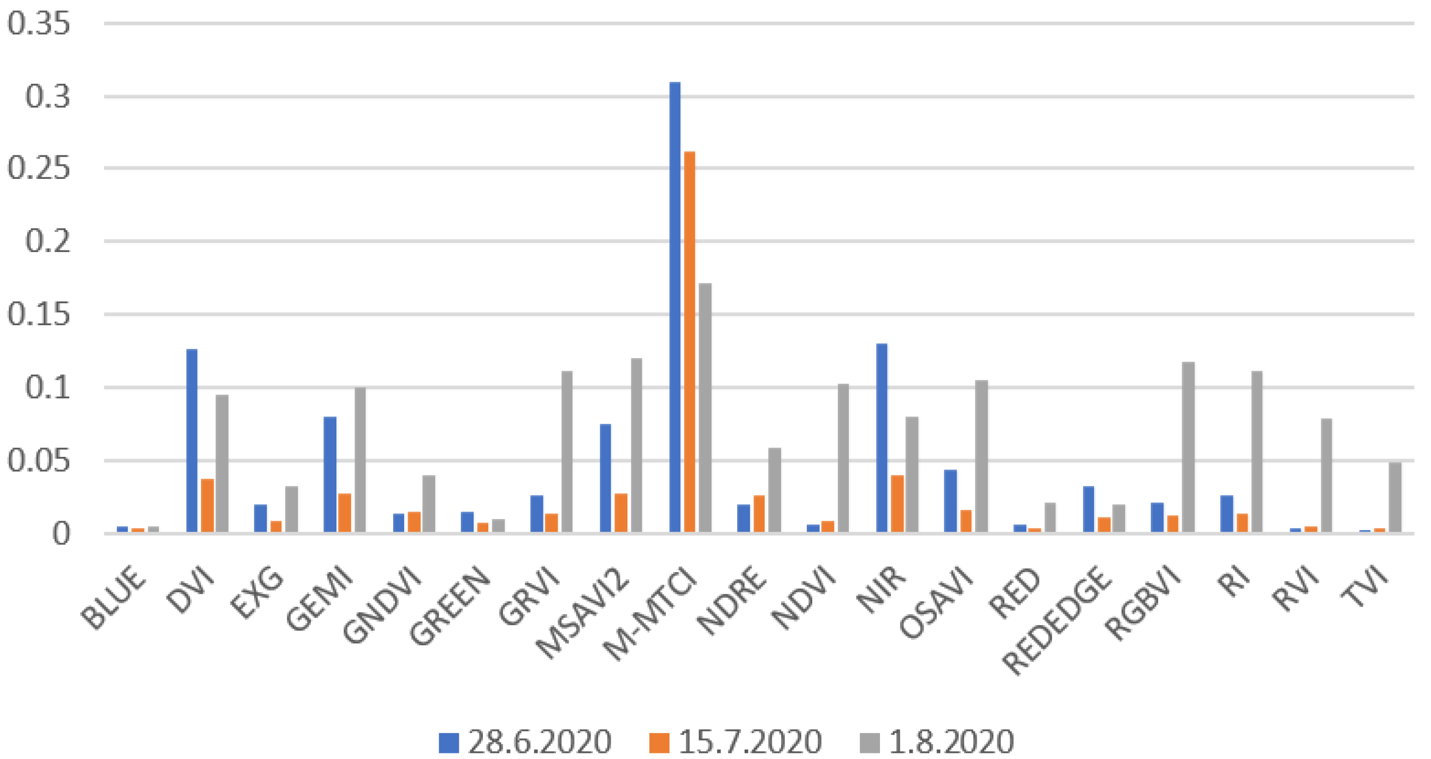
2.8. Variation in Vegetation Indices

The vegetation indices have different maximum and minimum values depending on their equations. Because of this, the coefficient of variation values were calculated to compare different vegetation indices with each other. The first step was to calculate each measurement point’s (Figure 3) reflectance/index values for each flight (8:00, 12:00, 16:00, and 20:00 flights). The second step was to calculate the coefficient of variation values for each measurement point between the different flight times for each spectral band/vegetation index. The last step was to calculate the average coefficient of variation from these 10 measurement points to present the vegetation index variation on one day. The calculation process is presented in Equation (3).

$$A=\left[\begin{array}{cccc}{k}_{1,1}& \dots & \dots & k_{1,j}\\ \dots & \dots & \dots & \dots \\ \dots & \dots & \dots & \dots \\ k_{i,1}& \dots & \dots & k_{10,4}\end{array} \right]\Rightarrow CV=mean\left(\frac{SD\left(A\right)}{mean\left(A\right)}\right)$$

(3)

where k is the vegetation index value, i is the number of the measurement point, and j corresponds to the flight event (time of the day). SD stands for standard deviation. In this study, there were 10 measurement points (i = 10) and four flight events at 8:00, 12:00, 16:00, and 20:00 (j = 4).

3. Results

3.1. Comparison of Vegetation Indices

Comparison of vegetation indices are represented in

Table 3. Coefficient of variation value for each vegetation index for every measurement day; 28 June had nine measurement points from which the coefficient of variation values were calculated. The other measurement days had ten points.

	Date	17.7.2019	31.7.2019	28.6.2020	15.7.2020	1.8.2020
Vegetation index	DVI	0.235	0.365	0.322	0.296	0.411
	EXG	0.213	0.534	0.346	0.353	0.318
	GEMI	0.108	0.205	0.149	0.179	0.209
	GNDVI	0.043	0.028	0.041	0.073	0.087
	GRVI	0.213	−0.495	0.084	0.092	−2.991
	MSAVI2	0.178	0.311	0.188	0.239	0.313
	M-MTCI	0.082	0.134	0.107	0.161	0.167
	NDRE	0.059	0.085	0.045	0.074	0.101
	NDVI	0.038	0.045	0.015	0.015	0.038
	OSAVI	0.089	0.174	0.117	0.141	0.187
	RGBVI	0.066	0.488	0.045	0.039	0.076
	RI	−0.213	0.495	−0.084	−0.092	2.991
	RVI	0.168	0.055	0.173	0.131	0.077
	TVI	0.012	0.011	0.005	0.005	0.010
	VIN	0.171	0.058	0.164	0.128	0.088

. The coefficient of variation values describe the variations in the vegetation indices within a day. Based on the results of Table 3, NDVI and TVI were least affected by the changes in solar radiation compared to other vegetation indices (changes were under 5% unit). For GNDVI, the changes were under 10% unit.

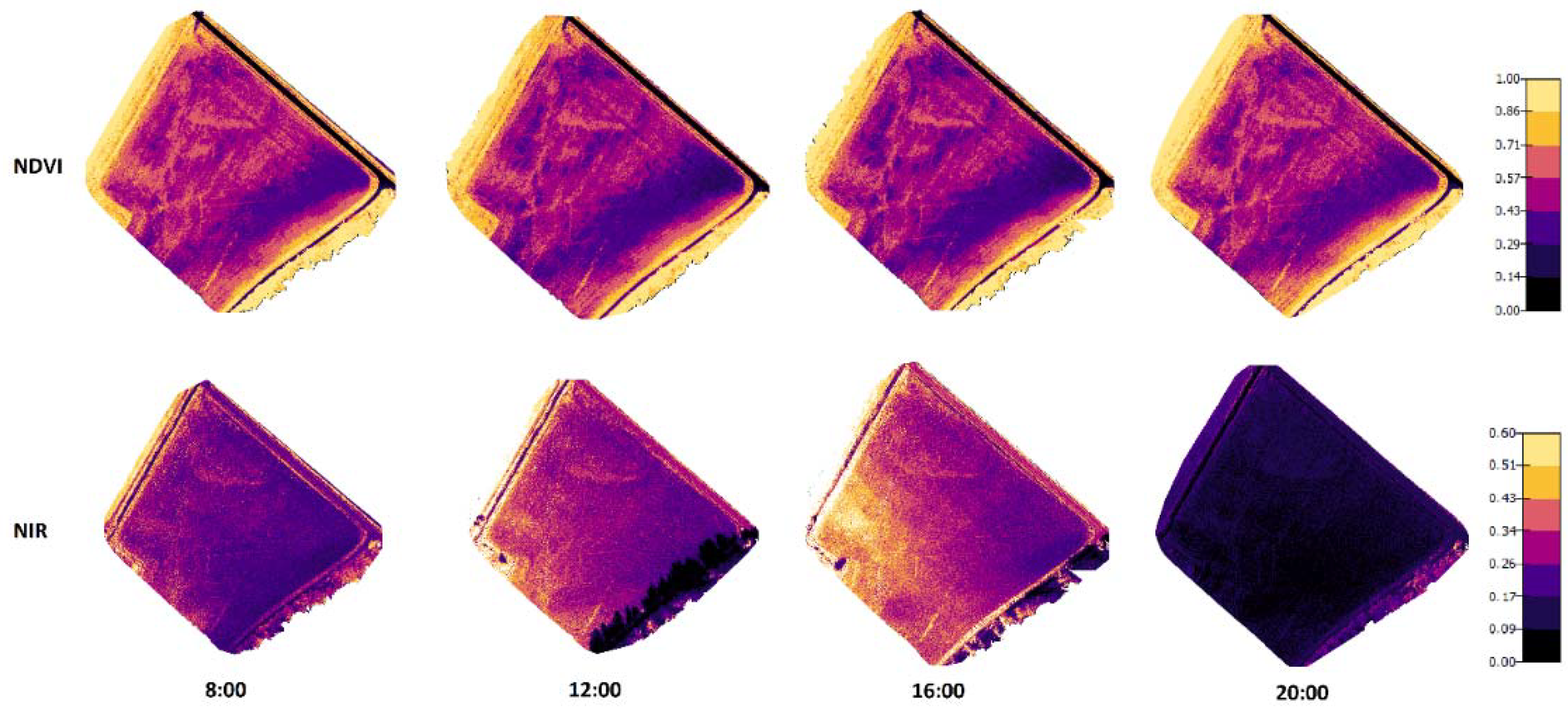
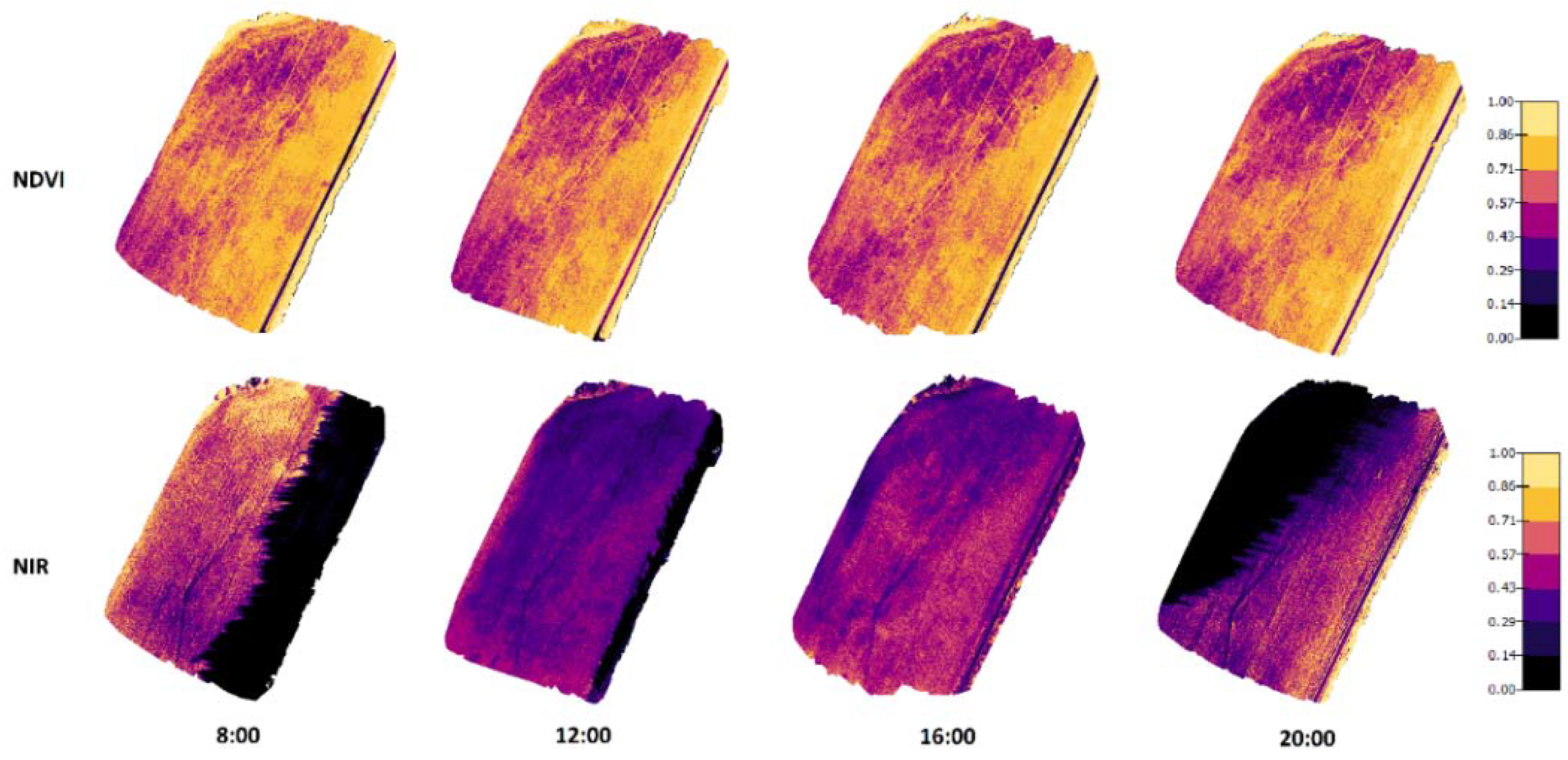
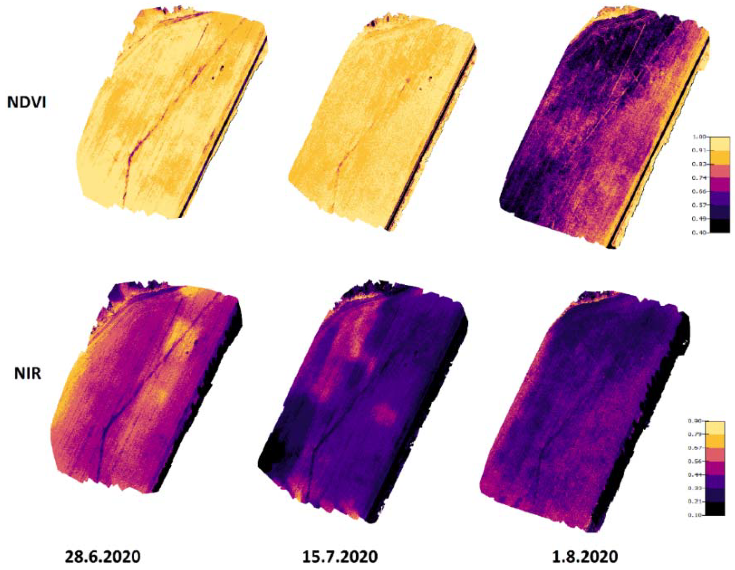
3.2. Orthomosaic Maps

Figure 6 and Figure 7 present the orthomosaic maps (geometrically correct aerial images) that were created from NIR and NDVI values of the crops in the two test fields. When comparing the NIR values in the images taken in 2019, there were noticeable dependencies on the lighting conditions and crop properties. On the other hand, the NDVI values were practically not influenced by the changing lighting conditions during the day, but different areas could be recognized in the figures with different crop properties.

The results presented in Figure 7 (created from the data recorded in 2020) have similar results to the 2019 measurements. There were significant shadows appearing in NIR images taken at 8:00 and 20:00. In these shadowed areas that existed on the east side in the morning and the west side in the evening, the NIR reflectance values were remarkably lower. Again, the NDVI values did not change a lot at different times, even the shadows did not have noticeable effects on the NDVI values.

Figure 8 presents NIR and NDVI maps from the 2020 measurements. From these images, the development of NIR and NDVI values can be seen during the growing season. NDVI values were quite high on 28 June and 15 July because the leaf areas were at their highest compared to the 1 August results when the crop started to ripen. NIR values were higher on 28 June compared to 15 July and 1 August. Higher NIR values for the 28 June measurements may have been caused by the rainless period in July causing dryer conditions (Figure 4). For the other two days, there were longer rain periods before the drone flights.

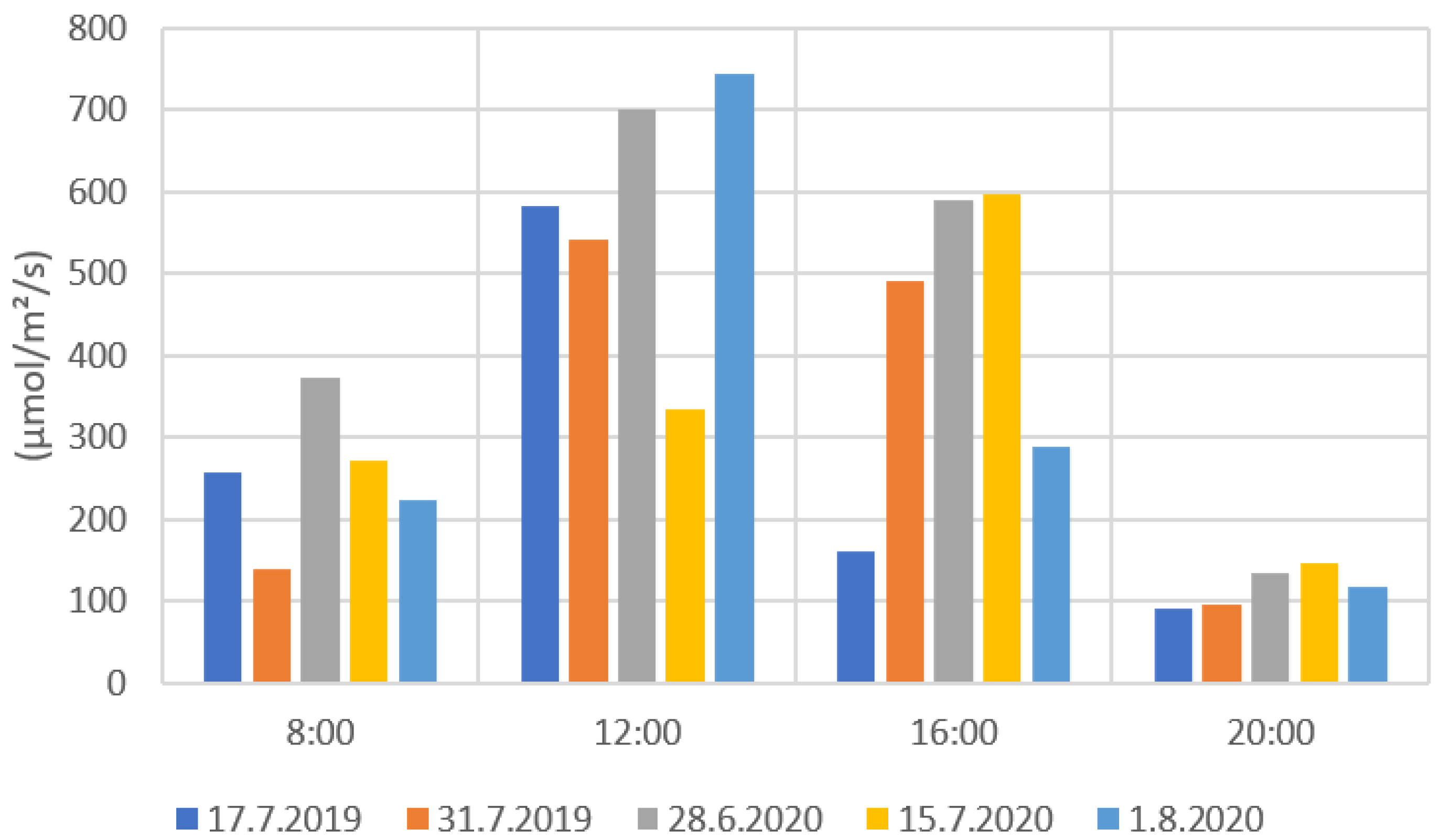
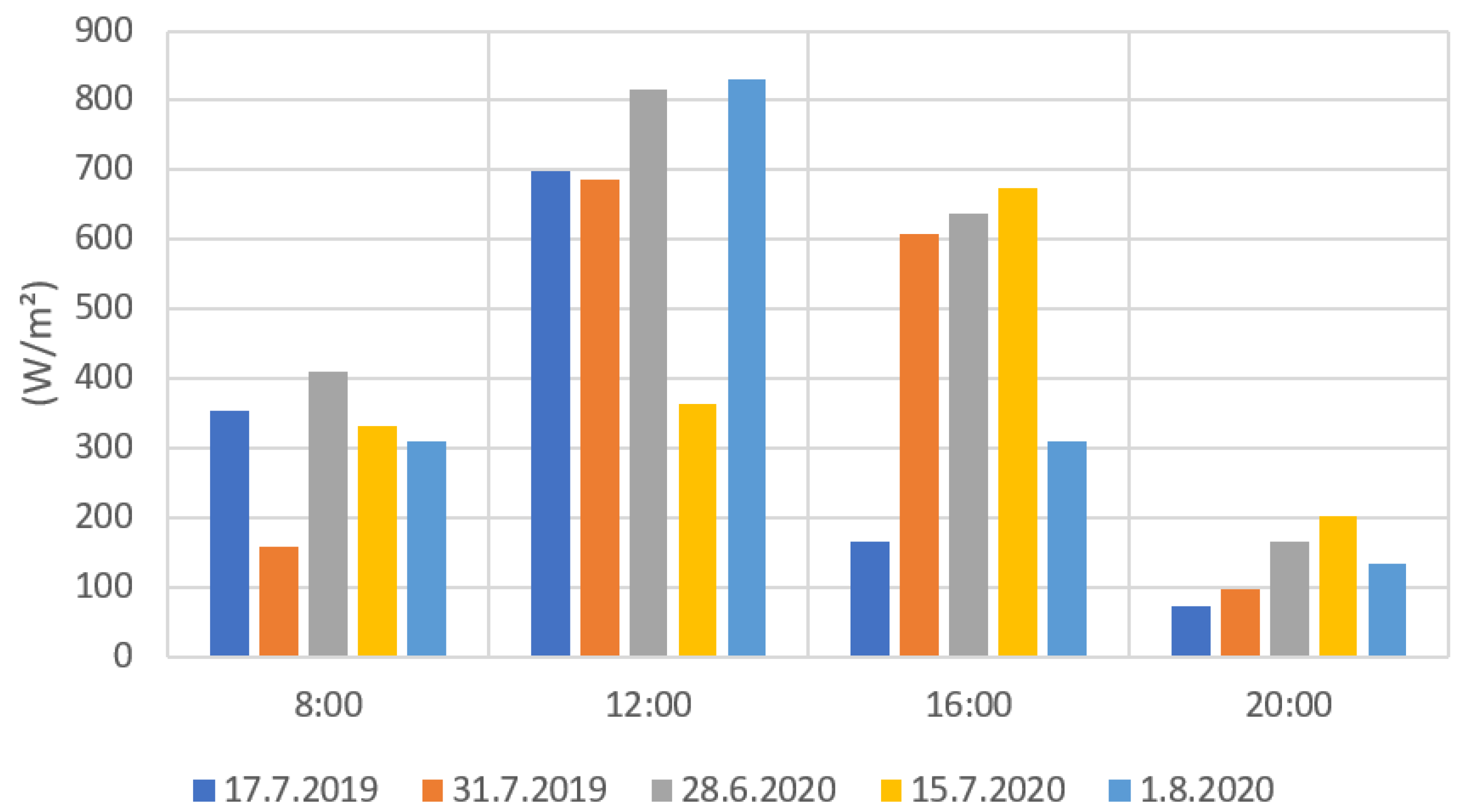
3.3. Solar Radiation

Figure 9 and Figure 10 present the results from the ground level solar radiation measurements during the drone flights. Both radiation values were notably higher during the measurements at 12:00 and 16:00 than at 8:00 and 20:00. The much lower radiation values in some measurements (e.g., 31 July 2019 at 12:00) were caused by the clouds preventing radiation to reach the ground. When comparing Figure 9 and Figure 10, the PYR and PAR results are very similarly distributed. This is due to that the measuring range of the PAR sensor being part of the measuring range of the PYR sensor. The PYR sensor measures radiation coming from a wider spectrum. The solar elevation has a clear effect on the solar radiation values. The 8:00 and 20:00 radiation values were clearly lower when the sun’s elevation values were also low (Appendix B,

Table A2. Solar position values for different flight days. Values were calculated using the NOAA ESRL (National Oceanic and Atmospheric Administration, Earth System Research Laboratories) calculator found on the internet: https://gml.noaa.gov/grad/solcalc/azel.html (accessed on 1 October 2021).

Date	Time		Solar Declination (Degrees)	Solar Azimuth (Degrees)	Solar Elevation (Degrees)	Solar Zenith Angle (Degrees)
17.7.2019		8	21.24	86.24	22.54	67.46
		12	21.21	144.22	47.14	42.86
		16	21.18	229.35	43.42	46.58
		20	21.15	283.79	16.62	73.38
31.7.2019		8	18.33	85.68	18.81	71.19
		12	18.29	148.92	45.07	44.93
		16	18.25	223	42.17	47.83
		20	18.21	280.27	15.22	74.78
28.6.2020		8	23.25	86.95	25.33	64.67
		12	23.24	153.47	51	39.00
		16	23.23	232.81	44.54	45.46
		20	23.22	286.92	17.22	72.78
15.7.2020		8	21.44	82.96	20.88	69.12
		12	21.42	146.46	47.84	42.16
		16	21.39	227.73	44.16	45.84
		20	21.36	282.47	17.62	72.38
1.8.2020		8	17.89	84.87	17.83	72.17
		12	17.85	149.45	44.72	45.28
		16	17.81	223.13	41.67	48.33
		20	17.77	278.16	15.93	74.07

).

3.4. Influence of the Crop on the Vegetation Indices

Figure 11 presents the standard deviation values calculated between the 10 measurement points. These results show the variations in reflectance/vegetation indices values caused by changes in the vegetation in the different areas of the field. The standard deviation values from different spectral bands/vegetation indices cannot always be compared with each other because their maximum and minimum values can vary a lot. Based on the growing stage, it seems that many of the vegetation indices (EXG, GEMI, GNDVI, GRVI, MSAVI2, NDRE, NDVI, OSAVI, RGBVI, RI, RVI, and TVI) reflected large in-field variations in crops on the last day of measurements (Figure 11). Some of the indices (blue, DVI, green, NIR, Rededge) did not show any regularities for the in-field variations. When looking at the five spectral bands, NIR had the largest standard deviation values and the most sensitive band of the multispectral camera to changes in the vegetation. NDVI’s deviation values were lower on 28 June and 15 July compared to the 1 August values. Higher deviations on the 1 August measurements could have been due to the ripened vegetation and the effect of the soil, which was more clearly visible at this time of the crop growth stage.

4. Discussion

Most of the aerial imaging research focuses on creating indicative values from the data acquired by a drone (to be used in crop monitoring) [18,39]. In many cases, multispectral or hyperspectral cameras are being used in data collections [40]. The purpose of this study was to delve deeper into multispectral imaging and analyze how the spectral bands and vegetation indices are affected by external factors. When taking images with a drone, there are multiple factors that can affect the values on multispectral images. Atmospheric effects have very low influences on drone images taken under 100 m of altitude [15].

Based on the measurements and analyzed results of this research, a couple of factors were found to affect the multispectral imaging. In the 2020 measurements, some of the measurement points were affected by shadows caused by the tree line. The NIR maps were clearly affected by the shadows, which resulted in lower reflectance values on the NIR spectral band, while the shadows did not have visual effects on the NDVI figures, being ratios of reflectance bands (Figure 7). This can be a problem, especially in Nordic conditions, where the sun elevation is low and the fields are located near forest areas. During the 8:00 measurements, dew occasionally formed on the vegetation. This could have also affected the multispectral images and the coefficient of variation values because wet and dry vegetations have different spectral values [41]. Another factor that may have affected the multispectral images was the soil surface. At the end of the growing season, the crop was ripened, and the soil surface had a greater effect on the multispectral images. The reflectance values from the soil surfaces were different than from the crops, and may have caused irregularities in the images [2]. Moreover, the changes in the soil moisture could have affected the multispectral images [42]. These kinds of disturbances could have affected the standard deviation values calculated in the results section.

The camera technology could affect the changes in values of the spectral bands and vegetation indices. The center wavelength, bandwidth, and other technical specs vary between cameras [2]. In Deng et al.’s [2] research, they compared two multispectral cameras. When they took images from the calibration panel, there were differences in the reflectance values between the cameras and between the images that were taken in cloudy and sunny weather. Therefore, it is crucial to carry out the calibration measures in the same field conditions as the measurements to ensure the correct image calibrations.

The colored maps in Section 3.2 illustrate well how the values of the vegetation indices change over time. The images were divided into five categories, but by adding more categories it will be possible to see smaller differences in the images. Figure 8 presents how NIR and NDVI values changed on the field during the growing season. Hassan et al. [7] studied changes in the NDVI values of wheat (Triticum aestivum) during the growing season. The results showed how the NDVI value of wheat increased up to the booting growth stage; after that, it started to decrease. In Yeom et al.’s [43] research, cotton and sorghum vegetation NDVI values increased at the beginning of the growing season and started to decrease after a certain growth stage. Similar results could be seen in this study with NDVI values of barley (Figure 8).

From the radiation measurements, it is possible to estimate the cloudiness of the weather for each measurement day. For example, in Figure 9 and Figure 10, the 15 July PYR and PAR measurements at 12:00 showed much lower values compared to other days at the 12:00 measurements. Lower PYR and PAR values indicated that there were clouds blocking the sun’s radiation when the drone images were taken. Similar results could be seen on 17 July 2019 and 1 August 2020 with the 16:00 measurements. In Finland, the field conditions can be challenging for drone imaging. Generally, in the northern latitudes, the sun’s elevation angle remains low during the growing season, and the radiation comes from a rather narrow angle. This is clearly visible in the 2020 measurements (Figure 7) when shadows were formed on the fields that were located near forests. Therefore, it would be beneficial to use vegetation indices that are the least affected by the changes in solar radiation and field conditions in general. These indices would also help to create models for crop monitoring that would not be so sensitive to changes in solar conditions.

From the standard deviation values in Section 3.4, it is possible to see how different vegetation indices and spectral bands reacts to changes in vegetation. Some of the vegetation indices, such as RGBVI and NDVI, had larger deviation values at the end of the growing season (Figure 11). The same phenomenon can be seen in NDVI maps in Figure 8. Toward the end of the growing season, there may have been more variations in the field due to crop ripening (and because the soil was more visible and could have affected the multispectral images). Marino and Alvino [39] used data clustering to classify wheat yields. In their research, they calculated the standard deviation for NDVI at three different crop stages. The results show how standard deviation values grow at the end of the growth season, which are in agreement with the results of this study (Figure 11).

Section 3.1 summarizes how much the vegetation indices are affected by the different weather conditions. The spectral bands were clearly affected by the weather conditions, but these effects could decrease by calculating different vegetation indices. Hashimoto et al. [44] simulated the reflectance and vegetation index values for paddy field monitoring. With the NDVI simulations, the values seemed to change very little or hardly at all when the sun’s zenith angle changed. The amount of diffused light had greater impact on NDVI values compared to the zenith angle. Red and NIR had greater changes in reflectance values when the zenith angle changed in the simulation. This study had similar results with NDVI, which was one of the least affected vegetation indices by the weather conditions (Table 3).

Some research studies have examined how the solar zenith angle affects the reflectance values of the spectral bands and vegetation indices. Ishihara et al. [45] measured how sunlight conditions affected NDVI and GRVI values. The largest changes in NDVI values were measured for rice where the values varied from 0.3 to 0.5 (when the zenith angle varied between 15 and 60°). For other crops (and for other measurement days) the variations in NDVI values were smaller. GRVI varied at the highest from 0.3 to 0.5 for rice. However, NDVI performed better than GRVI, which was also found in this study. In Li et al.’s [46] research, they measured how BRF (bi-directional reflectance) values changed with different solar zenith angles and viewing angles. At a 675 nm wavelength (red spectral band) the largest changes in BRF values from different zenith angles varied between 0.06 and 0.20 for sunflowers. At a 850 nm wavelength (NIR spectral band) the largest changes varied between 0.3 and 0.47 for sunflowers. The viewing angle affected the BRF values; the greatest was from 0.06 to 0.20 for a 675 nm wavelength and 0.15 to 0.45 for a 850 nm wavelength. The results clearly show how the solar zenith and the viewing angle affect the reflected values for these two spectral bands. In this study, similar results were found for NIR and red spectral bands. The difference in this study is that orthomosaic maps were used instead of individual multispectral images. Therefore, the measurement point values are a combination from multiple pictures taken from different viewing angles. The Pix4D software used to create orthomosaic maps does not have bidirectional reflectance distribution functions (BRDF).

Currently, there are very few studies that compare the field condition effects and vegetation indices. The advantage of this research is that multiple vegetation indices were compared. Most of the research focused on using one or multiple vegetation indices to describe the crop properties, such as yield or chlorophyll content at the time when the pictures were taken [8,17]. Further research could be conducted on how these different factors affect the reflectance and vegetation index values.

5. Conclusions

Multispectral image and weather data were collected during two growing seasons. From the multispectral images, 15 vegetation indices were calculated for a more detailed inspection. This study examined how the vegetation indices and values of spectral bands changed on the field at different times of the day. Among the vegetation indices, NDVI was minorly affected by the field conditions, and the mean and standard deviation values for NDVI were similar between different measurements. NDVI and TVI performed the best out of the vegetation indices, with coefficients of variation value under 5%.

Overall, the results analysis clearly indicates that in Nordic conditions, the lighting conditions should be carefully considered when carrying out aerial imaging with multispectral cameras. It was also concluded that vegetation indices respond differently to the changes in lighting conditions due to large variations involving the use of spectral bands when calculating vegetation indices. It was observed that the NIR spectral band was positively impacted by mitigating the changes caused by the field conditions. Further research could (and should) be conducted on how the changes in spectral reflectance values could be automatically corrected. This could help improve the accuracy of vegetation indices that are used for specific tasks, such as soil moisture monitoring. Multiple vegetation indices could also be tested on how different weather conditions affect their values.

References

1. Kim, J.; Kim, S.; Ju, C.; Son, H.I. Unmanned Aerial Vehicles in Agriculture: A Review of Perspective of Platform, Control, and Applications. IEEE Access 2019, 7, 105100–105115. [Google Scholar] [CrossRef]
2. Deng, L.; Mao, Z.; Li, X.; Hu, Z.; Duan, F.; Yana, Y. UAV-based multispectral remote sensing for precision agriculture: A comparison between different cameras. ISPRS J. Photogramm. Remote Sens. 2018, 146, 124–136. [Google Scholar] [CrossRef]
3. Shendryk, Y.; Sofonia, J.; Garrard, R.; Rist, Y.; Skocaj, D.; Thorburn, P. Fine-scale prediction of biomass and leaf nitrogen content in sugarcane using UAV LiDAR and multispectral imaging. Int. J. Appl. Earth Obs. Geoinf. 2020, 92, 102177. [Google Scholar] [CrossRef]
4. Xu, X.; Fan, L.; Li, Z.; Meng, Y.; Feng, H.; Yang, H.; Xu, B. Estimating Leaf Nitrogen Content in Corn Based on Information Fusion of Multiple-Sensor Imagery from UAV. Remote Sens. 2021, 13, 340. [Google Scholar] [CrossRef]
5. Xie, T.; Li, J.; Yang, C.; Jiang, Z.; Chen, Y.; Guo, L.; Zhang, J. Crop height estimation based on UAV images: Methods, errors, and strategies. Comput. Electron. Agric. 2021, 185, 106155. [Google Scholar] [CrossRef]
6. Kerkech, M.; Hafiane, A.; Canals, R. Vine disease detection in UAV multispectral images using optimized image registration and deep learning segmentation approach. Comput. Electron. Agric. 2020, 174, 105446. [Google Scholar] [CrossRef]
7. Hassan, M.A.; Yang, M.; Rasheed, A.; Yang, G.; Reynolds, M.; Xia, X.; Xiao, Y.; He, Z. A rapid monitoring of NDVI across the wheat growth cycle for grain yield prediction using a multi-spectral UAV platform. Plant Sci. 2019, 282, 95–103. [Google Scholar] [CrossRef]
8. Qi, H.; Wu, Z.; Zhang, L.; Li, J.; Zhou, J.; Jun, Z.; Zhu, B. Monitoring of peanut leaves chlorophyll content based on drone-based multispectral image feature extraction. Comput. Electron. Agric. 2021, 187, 106292. [Google Scholar] [CrossRef]
9. Mazzia, V.; Comba, L.; Khaliq, A.; Chiaberge, M.; Gay, P. UAV and Machine Learning Based Refinement of a Satellite-Driven Vegetation Index for Precision Agriculture. Sensors 2020, 20, 2530. [Google Scholar] [CrossRef] [PubMed]
10. Qian, W.; Huang, Y.; Liu, Q.; Fan, W.; Sun, Z.; Dong, H.; Wan, F.; Qiao, X. UAV and a deep convolutional neural network for monitoring invasive alien plants in the wild. Comput. Electron. Agric. 2020, 174, 105519. [Google Scholar] [CrossRef]
11. Cao, Y.; Li, G.L.; Luo, Y.K.; Pan, Q.; Zhang, S.Y. Monitoring of sugar beet growth indicators using wide-dynamic-range vegetation index (WDRVI) derived from UAV multispectral images. Comput. Electron. Agric. 2020, 171, 105331. [Google Scholar] [CrossRef]
12. Kaufman, Y.; Tanre, D. Atmospherically resistant vegetation index (ARVI) for EOS-MODIS. IEEE Trans. Geosci. Remote Sens. 1992, 30, 261–270. [Google Scholar] [CrossRef]
13. Huete, A.; Justice, C.; Liu, H. Development of vegetation and soil indices for MODIS-EOS. Remote Sens. Environ. 1994, 49, 224–234. [Google Scholar] [CrossRef]
14. Fitzgeralda, G.; Rodriguezb, D.; O’Learya, G. Measuring and predicting canopy nitrogen nutrition in wheat using a spectral index—The canopy chlorophyll content index (CCCI). Field Crops Res. 2010, 116, 318–324. [Google Scholar] [CrossRef]
15. Guo, Y.; Senthilnath, J.; Wu, W.; Zhang, X.; Zeng, Z.; Huang, H. Radiometric Calibration for Multispectral Camera of Different Imaging Conditions Mounted on a UAV Platform. Sustainability 2019, 11, 978. [Google Scholar] [CrossRef]
16. Näsi, R.; Viljanen, N.; Kaivosoja, J.; Alhonoja, K.; Hakala, T.; Markelin, L.; Honka-vaara, E. Estimating Biomass and Nitrogen Amount of Barley and Grass Using UAV and Aircraft Based Spectral and Photogrammetric 3D Features. Remote Sens. 2018, 10, 1082. [Google Scholar] [CrossRef]
17. Viljanen, N.; Honkavaara, E.; Näsi, R.; Hakala, T.; Niemeläinen, O.; Kaivosoja, J. Novel Machine Learning Method for Estimating Biomass of Grass Swards Using a Photogrammetric Canopy Height Model, Images and Vegetation Indices Captured by a Drone. Agriculture 2018, 8, 70. [Google Scholar] [CrossRef]
18. Wu, C.; Niu, Z.; Tang, Q.; Huang, W. Estimating chlorophyll content from hyperspectral vegetation indices: Modeling and validation. Agric. For. Meteorol. 2008, 148, 1230–1241. [Google Scholar] [CrossRef]
19. Rouse, J.W.; Haas, R.H.; Schell, J.A.; Deering, D.W. Monitoring Vegetation Systems in the Great Plains with ERTS. In Third ERTS-1 Symposium; NASA SP-351: Washington, DC, USA, 1974; pp. 309–317. [Google Scholar]
20. Carlson, T.; Ripley, D.A. On the relation between NDVI, fractional vegetation cover, and leaf area index. Remote Sens. Environ. 1997, 62, 241–252. [Google Scholar] [CrossRef]
21. Suab, S.A.; Syukur, M.S.B.; Avtar, R.; Korom, A. Unmanned aerial vehicle (uav) derived normalised difference vegetation index (ndvi) and crown projection area (cpa) to detect health conditions of young oil palm trees for precision agriculture. In Proceedings of the 6th International Conference on Geomatics and Geospatial Technology (GGT 2019), Kuala Lumpur, Malaysia, 1–3 October 2019. [Google Scholar]
22. Lu, J.; Cheng, D.; Geng, C.; Zhang, Z.; Xiang, Y.; Hu, T. Combining plant height, canopy coverage and vegetation index from UAV-based RGB images to estimate leaf nitrogen concentration of summer maize. Biosyst. Eng. 2021, 202, 42–54. [Google Scholar] [CrossRef]
23. Maimaitijiang, M.; Sagana, V.; Sidikea, P.; Hartling, S.; Esposito, F.; Fritschid, F. Soybean yield prediction from UAV using multimodal data fusion and deep learning. Remote Sens. Environ. 2020, 237, 111599. [Google Scholar] [CrossRef]
24. Noguera, M.; Aquino, A.; Ponce, J.M.; Cordeiro, A.; Silvestre, J.; Arias-Calderon, R.; Marcelo, M.; Jordao, P.; Andujar, J.M. Nutritional status assessment of olive crops by means of the analysis and modelling of multispectral images taken with UAVs. Biosyst. Eng. 2021, 211, 1–18. [Google Scholar] [CrossRef]
25. Zadoks, J.C.; Chang, T.T.; Konzak, C.F. A decimal code for the growth stages of cereals. Weed Res. 1974, 14, 415–421. [Google Scholar] [CrossRef]
26. Finnish Meteorological Institute. Precipitation Amount and Air Temperature. Available online: https://en.ilmatieteenlaitos.fi/download-observations (accessed on 1 October 2021).
27. Richardson, A.J.; Wiegand, C.L. Distinguishing vegetation from soil background information. Photogramm. Eng. Remote Sens. 1977, 43, 1541–1552. [Google Scholar]
28. Woebbecke, D.M.; Meyer, G.E.; Von Bargen, K.; Mortensen, D.A. Color Indices for Weed Identification Under Various Soil, Residue, and Lighting Conditions. Trans. ASAE 1995, 38, 259–269. [Google Scholar] [CrossRef]
29. Pinty, B.; Verstraete, M.M. GEMI: A non-linear index to monitor global vegetation from satellites. Vegetatio 1992, 101, 15–20. [Google Scholar] [CrossRef]
30. Gitelson, A.; Merzlyak, M. Quantitative estimation of chlorophyll a using reflectance spectra: Experiments with autumn chestnut and maple leaves. J. Photochem. Photobioliology B Biol. 1994, 22, 247–252. [Google Scholar] [CrossRef]
31. Tucker, C. Red and photographic infrared linear combinations formonitoring vegetation. Remote Sens. Environ. 1979, 8, 127–150. [Google Scholar] [CrossRef]
32. Dash, J.; Curran, P. The MERIS terrestrial chlorophyll index. Int. J. Remote Sens. 2004, 25, 5403–5413. [Google Scholar] [CrossRef]
33. Qi, J.; Chehbouni, A.; Huete, A.; Kerr, Y.; Sorooshian, S. A modified soil adjusted vegetation index. Remote Sens. Environ. 1994, 48, 119–126. [Google Scholar] [CrossRef]
34. Rondeaux, G.; Steven, M.; Baret, F. Optimization of soil-adjusted vegetation indices. Remote Sens. Environ. 1996, 55, 95–107. [Google Scholar] [CrossRef]
35. Bendig, J.; Yu, K.; Aasen, H.; Bolten, A.; Bennertz, S.; Broscheit, J.; Gnyp, M.; Bareth, G. Combining UAV-based plant height from crop surface models, visible and near infrared vegetation indices for biomass monitoring in barley. Int. J. Appl. Earth Obs. Geoinf. 2015, 39, 79–87. [Google Scholar] [CrossRef]
36. Escadafal, R.; Huete, A.R. Étude des propriétés spectrales des sols arides appliquée à l’amélioration des indices de végétation obtenus par télédétection. CR Acad. Sci. 1991, 312, 1385–1391. [Google Scholar]
37. Pearson, R.L.; Miller, L.D. Remote mapping of standing crop biomass for estimation of the productivity of the shortgrass prairie, Pawnee National Grasslands, Colorado. In Proceedings of the 8th International Symposium on Remote Sensing of the Environment II, Ann Arbor, MI, USA, 2–6 October 1972; pp. 1355–1379. [Google Scholar]
38. Rouse, J.W.; Haas, R.H.; Schell, J.A.; Deering, D.W.; Harlan, J.C. Monitoring the Vernal Advancement and Retrogradation (Greenwave Effect) of Natural Vegetation; Report RSC 1978-4; Texas A&M University, Remote Sensing Center: College Station, TX, USA, 1974. [Google Scholar]
39. Marino, S.; Alvino, A. Vegetation Indices Data Clustering for Dynamic Monitoring and Classification of Wheat Yield Crop Traits. Remote Sens. 2021, 13, 541. [Google Scholar] [CrossRef]
40. Candiago, S.; Remondino, F.; De Giglio, M.; Dubbini, M.; Gattelli, M. Evaluating Multispectral Images and Vegetation Indices for Precision Farming Applications from UAV Images. Remote Sens. 2015, 7, 4026–4047. [Google Scholar] [CrossRef]
41. Zhang, F.; Zhou, G. Estimation of vegetation water content using hyperspectral vegetation indices: A comparison of crop water indicators in response to water stress treatments for summer maize. BMC Ecol. 2019, 19, 18. [Google Scholar] [CrossRef]
42. Weidong, L.; Bareta, F.; Xingfaa, G.; Qingxib, T.; Lanfenb, Z.; Bingb, Z. Relating soil surface moisture to reflectance. Remote Sens. Environ. 2002, 81, 238–246. [Google Scholar] [CrossRef]
43. Yeom, J.; Jung, J.; Chang, A.; Ashapure, A.; Maeda, M.; Maeda, A.; Landivar, J. Comparison of Vegetation Indices Derived from UAV Data for Differentiation of Tillage Effects in Agriculture. Remote Sens. 2019, 11, 1548. [Google Scholar] [CrossRef]
44. Hashimoto, N.; Saito, Y.; Maki, M.; Homma, K. Simulation of Reflectance and Vegetation Indices for Unmanned Aerial Vehicle (UAV) Monitoring of Paddy Fields. Remote Sens. 2019, 11, 2119. [Google Scholar] [CrossRef]
45. Ishihara, M.; Inoue, Y.; Ono, K.; Shimizu, M.; Matsuura, S. The Impact of Sunlight Conditions on the Consistency of Vegetation Indices in Croplands—Effective Usage of Vegetation Indices from Continuous Ground-Based Spectral Measurements. Remote Sens. 2015, 7, 14079–14098. [Google Scholar] [CrossRef]
46. Li, W.; Jiang, J.; Weiss, M.; Madec, S.; Tison, F.; Philippe, B.; Comar, A.; Baret, F. Impact of the reproductive organs on crop BRDF as observed from a UAV. Remote Sens. Environ. 2021, 259, 112433. [Google Scholar] [CrossRef]
Figure 1. Custom-built drone with a Tarot T960 frame. The multispectral camera light sensor had a separate gimbal (small figure). This solution minimizes disturbances that are caused by shadows forming on the sensor when the drone is flying away from the sun.
Remotesensing 14 04792 g001
Figure 2. Research fields are marked with yellow stripes on the picture. The upper field is named Mölylä and the other field is Koirasuo. The picture is from Google Earth, June 2020.
Remotesensing 14 04792 g002
Figure 3. Orthomosaic pictures from the NIR spectral band. In the images, the multiple white squares are the ten measurement points of the crop properties. The image of the Mölylä field (left) was taken on 31 July 2019 at 12:00 and the image of the Koirasuo field (right) on 1 August 2020 at 12:00.
Remotesensing 14 04792 g003
Figure 4. Accumulated rainfall (mm) and effective temperature sum (°C d) for both measurement years. The effective temperature sum was calculated by measuring the average temperature of each day, subtracting 5 °C from it, and summing the positive differences with each other. The flight days are marked as dots.
Remotesensing 14 04792 g004
Figure 5. Process diagram of the work steps in this study.
Remotesensing 14 04792 g005
Figure 6. Orthomosaic maps for NDVI and NIR values of the Mölylä field at four measurement times. The measurements were taken on 31 July 2019 when the crop growth stage on spring barley was 87 (Zadoks value).
Remotesensing 14 04792 g006
Figure 7. Orthomosaic maps for NDVI and NIR values in Koirasuo field at four different measurement times. The measurements were taken on 1 August 2020 when the crop growth stage for spring barley was 86 (Zadoks value).
Remotesensing 14 04792 g007
Figure 8. NIR and NDVI development on Koirasuo field during the growing season in 2020. The Zadoks values were 69 (28.6), 83 (15.7), and 86 (1.8). The orthomosaic maps were created from pictures taken at 12:00.
Remotesensing 14 04792 g008
Figure 9. PYR radiation measurement results for each flight date.
Remotesensing 14 04792 g009
Figure 10. PAR radiation measurement values for each flight date.
Remotesensing 14 04792 g010
Figure 11. Standard deviations between the ten (15.7 and 1.8.2020) and nine (28.6.2020) measurements points for each spectral band/vegetation index. These values were calculated from 16:00 measurements. Zadoks values were 69 (28.6), 83 (15.7), and 86 (1.8). VIN vegetation index standard deviation values were not included in this image because they were so large and made it difficult to read other values. VIN standard deviation values for 16:00 measurements were 2.41 (28 June 2020), 1.20 (15 July 2020), and 1.71 (1 August 2020).
Remotesensing 14 04792 g011