Detection of Waste Plastics in the Environment: Application of Copernicus Earth Observation Data

Abstract

The detection of waste plastics in the marine and terrestrial environment using satellite Earth Observation data offers the possibility of large-scale mapping and reducing on-the-ground manual investigation. In addition, costs are kept to a minimum by utilizing free-to-access Copernicus data. A Machine Learning-based classifier was developed to run on Sentinel-1 and -2 data. In support of the training and validation, a dataset was created with terrestrial and aquatic cases by manually digitizing varying landcover classes alongside plastics under the sub-categories of greenhouses, plastic, tyres and waste sites. The trained classifier, including an Artificial Neural Network and post-processing decision tree, was verified using five locations encompassing these different forms of plastic. Although exact matchups are challenging to digitize, the performance has generated high accuracy statistics, and the resulting land cover classifications have been used to map the occurrence of plastic waste in aquatic and terrestrial environments.

1. Introduction

The presence of plastics in the environment is of increasing concern and a pressing environmental issue, with incorrect disposal resulting in the contamination of marine, terrestrial and airborne environments. In addition, when plastics are exposed to ambient solar radiation, they slowly disintegrate into microplastics and release greenhouse gases, methane and ethylene [1]. Some facts of concern are that [2]: half of all manufactured plastics have been made in the last 15 years, and production has increased exponentially, from 2.3 million tons in 1950 to 448 million tons by 2015. Additionally, the mass of plastics is twice that of animate creatures inhabiting planet earth [3]. With an awareness of how plastic harms the environment, its mapping and recovery is an increasing focus alongside using less plastic in our everyday lives.

The everyday use of plastic bags and other single-use plastic products is widespread in many countries. Additionally, countries can have specific sources of plastics; e.g., in Nigeria, the packaging of drinking water in plastic is omnipresent [4]. Combined with this, waste management can be a significant problem due to a lack of recycling infrastructure, trained workforce, and other related factors. In addition, where facilities are available illegal fly-tipping can occur when those involved try to avoid disposal fees, e.g., the fly-tipping statistics for England in 2020/21 compared to 2019/20 showed a 16% increase with the primary source being household waste [5]. Additional concerns have arisen concerning waste materials being wrapped in plastics and disguised as other forms of legal waste, such as silage bales, which increases the difficulty of illegal waste detection and regulation enforcement [6,7].

In agriculture, plastics have become indispensable and are highly visible when used for crop protection and shading, such as greenhouses and ground covering films, and large plastic bales holding silage—termed plasticulture. However, in Europe, there are often inefficient management schemes, with data on the use of plastics in agriculture challenging to obtain [8].

Stockpiles of waste tyres have been identified as a significant danger to human and environmental health [6]. Before the introduction of the European Union’s Waste Framework Directive (2008/98/EC) [9], it was estimated over a billion tyres existed in poorly managed or unmanaged stockpiles across Europe [10]. Globally, it is estimated that one billion end-of-life tyres are created annually, and approximately four billion are in stockpiles and landfills [11].

The environmental harm caused by waste plastics is not only to the location where the plastics are used/dumped, as they can end up in waterways that take them out to sea. During their transport in aquatic systems, fresh plastics are gradually broken down into microplastics (<5 mm in diameter) and nanoplastics (<1 μm) [12]. It is estimated that about 150 million tonnes of plastic debris circulate in the world’s oceans [13].

Earth Observation (EO) data have the potential to detect plastics as they have a spectral signature that can be separated from the surrounding land cover types. For plastic waste floating on water, both Biermann et al. [14] and Themistocleous et al. [15] used indices derived from Sentinel-2 data; the Floating Debris Index and Plastic Index use the near-infrared (NIR) and red bands. The advantage of floating plastic is that the plastics are bright compared to the background, which is no longer true when plastics are on land as the background landcover can also have variable bright targets such as reflective roofs. Additionally, separating the detection of waste from the intended presence of plastics in the terrestrial environment can be difficult as it is present in greenhouses, synthetic turf and on the rooves of buildings as plastic roof tiles. However, the bright surface signatures of windrows (litter accumulation due to convergence zones in the ocean) may not only be due to the accumulation of plastics [16].

Amongst 33 polymers reported in the Indian coastal environment, polyethylene and polypropylene were the most dominant type in the sediment, water, and biota [17]. In plasticulture, polyethylene is popular as it’s a white semitransparent plastic with a spectral reflectance strongly influenced by the soil/vegetation characteristics it covers. However, plastic-mulched farmland is brighter, smoother (because it reduces soil roughness) and drier (it has low vapor and air permeability and low water absorbability) than other classes. So, the reflectance of plastic-mulched farmland has higher reflectance values in the shortwave infrared (SWIR) bands [18]. Levin et al. [19] used absorption features at 1218 and 1732 nm to detect plastic features associated with plasticulture. Similarly, for floating plastic waste, Goddijn-Murphy and Dufaur [20] noted absorption peaks at around 1140 and 1680 nm.

Guffogg et al. [21] noted that an obstacle for spectral detection on some beaches was that a large percentage of the plastic debris was shoes, predominantly flip flops, with polyurethane foam not having received as much focus as other plastics. They found that between 2–8%, depending on the plastic polymer, of a unit area must be covered in plastics before the material can be spectrally separated from a non-contaminated area only containing sand.

The detection of municipal or illegal waste sites on land has received less attention, although they are a recognized source of poorly managed marine pollution. Page et al. [22] is the previous version of this paper’s approach, which classified tyre and plastic waste in Scotland using Sentinel-1 and Sentinel-2 data. Kruse et al. [23] focused on plastic aggregation sites across Indonesia. They found that the centres of 19% of waste sites in Southeast Asia are located within 200 m of a waterway or waterbody listed on OpenStreetMap, and more than half are within 750 m. Gill et al. [24] used Landsat thermal data due to the heat generation in landfills; in comparison to the immediate surroundings, higher Land Surface Temperature (LST) values of a few Kelvin were reported within the study landfill site [25]. They developed an analytical framework for screening illegal dump sites using night-time light from Suomi VIIRS satellite imagery as a proxy. Karimi et al. [26] combined night-time light imagery with LST and modified soil adjusted index alongside vector layers for highways, railways and disposal sites. The night-time satellite imagery was used to determine populated areas [26].

Considering the approaches implemented previously, the objective of this study was to develop a method for automatically detecting a variety of plastic waste across aquatic and terrestrial environments from EO satellite data to provide a viable approach for repeatable, cost-effective, and large-scale monitoring. More specifically, this study assessed the suitability of a Sentinel-1 and -2 synergy product for plastic waste detection using a Keras implemented Sequential model to define an Artificial Neural Network (ANN); Keras is a high-level API that runs on top of TensorFlow for this Python implementation.

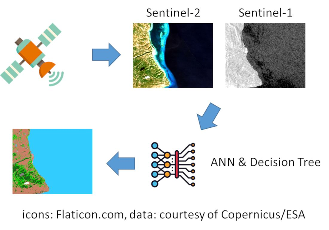
2. Materials and Methods

In this study, five test sites have been used to showcase the accuracy of the detection of plastics in different environments. A classifier has been developed with a pre-processing step that processes the input satellite data such that it is suitable for the stack of layers supplied to the Neural Network classifier. Then, a post Neural Network Decision Tree is applied to refine the generated land cover classification before several accuracy measures are used to understand the classifier’s ability to detect plastic waste within different scenarios.

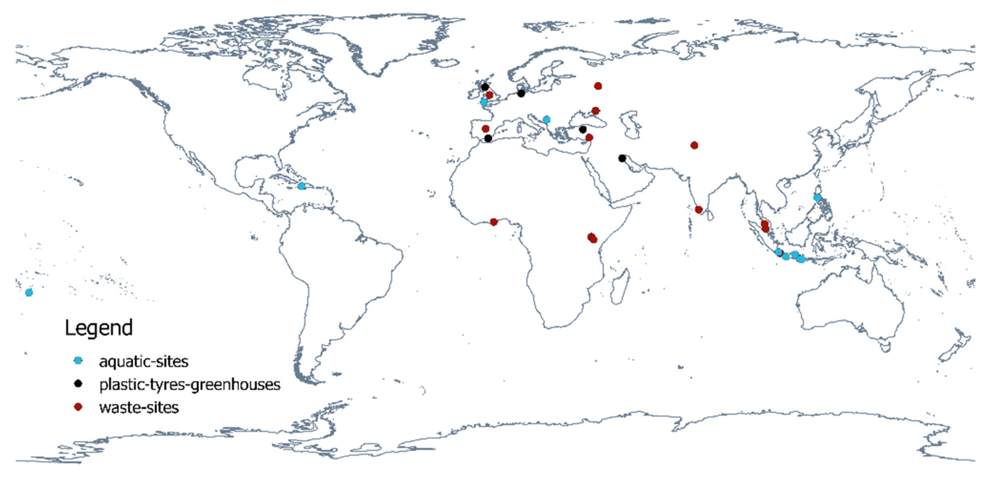
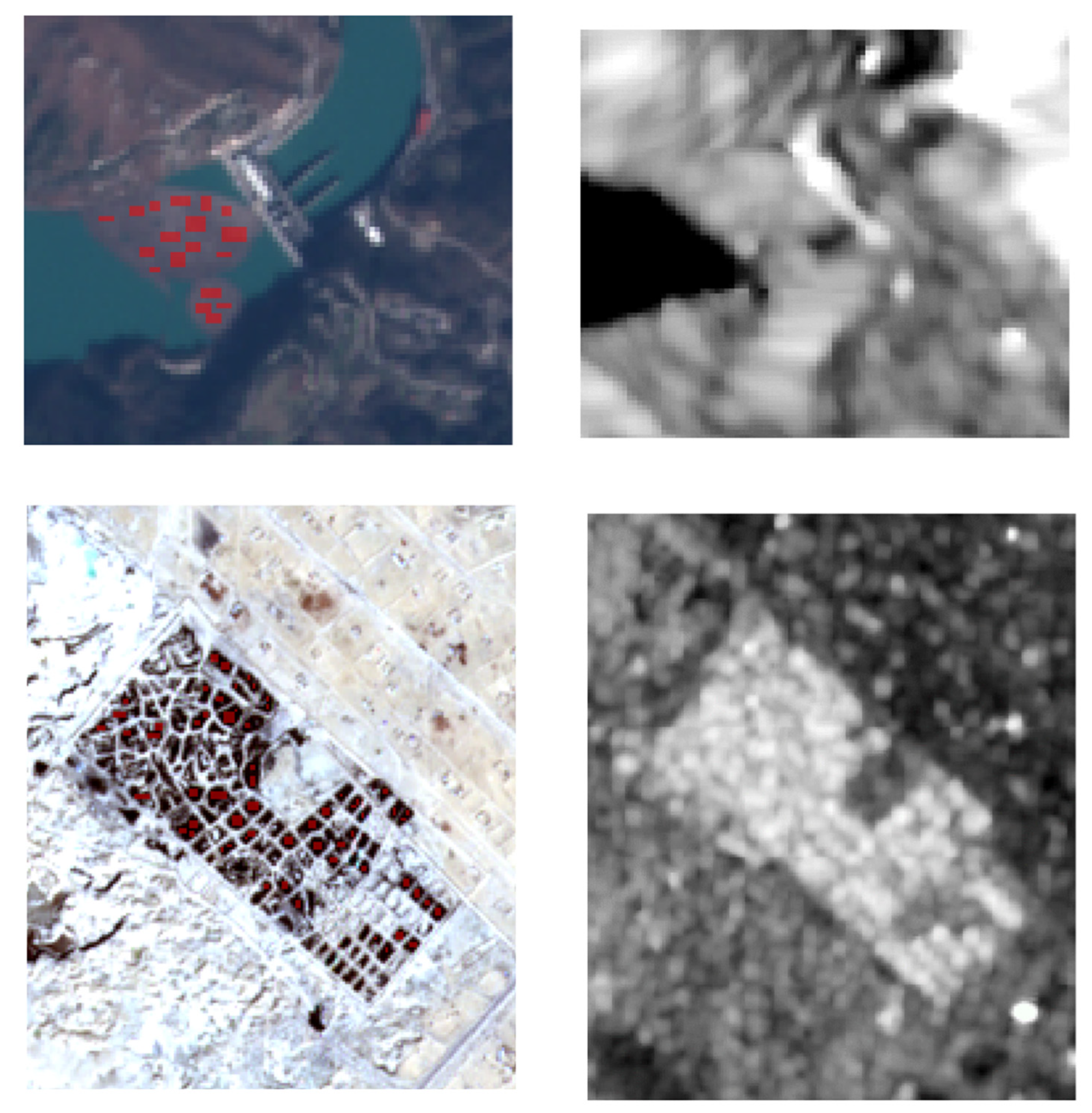
2.1. Test Sites and Input Satellite Products

Five test sites with different types of plastic pollution are being used to demonstrate the performance of the developed classifier for automatically detecting plastic waste. The Sentinel-1 Interferometric Wide Swath (IW) Ground Range Detected High Resolution (GRDH) and Sentinel-2 Level-2A (L2A, atmospherically corrected) files used for the plastic waste detection are shown in

Table 1. Test site locations with Sentinel-1 IW GRDH and Sentinel-2 Level 2A files as date/time and (for Sentinel-2) tile.

Test Site (Co-Ordinates)	Sentinel-1 IW GRDH	Sentinel-2 L2A
Višegrad Dam (43°45′35.62″N 19°17′15.68″E)	S1A 20210302T163318	S2A 20210302T09303 T34TCP *
Solo River Mouth (6°50′57.89″S 112°34′33.44″E)	S1A 20210218T220906 & 20210218T220931 **	S2A 20210227T023641 T49MFN
Srinagar Landfill (34°7′28.81″N 74°47′11.60″E)	S1A 20211031T005910	S2A 20211029T053941 T43SDT
Tyre Graveyard (29°15′24.42″N 47°40′22.96″E)	S1A 20201228T024734 & 20201228T024709 **	S2A 20201226T073321 T38RQT
Almería Greenhouses (36°43′6.72″N 2°45′12.82″W)	S1A 20210408T061050	S2A 20210505T105031 T30SWF

* Processed from Level 1C to Level 2A as there were issues using the online Level 2 file. ** Two Sentinel-1 files merged to cover the area of interest for the test site fully

.

The Sentinel-2 files are from 2021, so they have a relatively consistent processing version between themselves and the training data. Version 2.09 became active on 4 February 2020 with improvements in the NO DATA masking, then version 3.00 on 30 March 2021 had improved geometry and masks. There was a major upgrade to version 4.0 on 25 January 2022, when the format and radiometry changed [27]. There will be a reprocessing activity in the future, so all files have consistent processing.

Sentinel-1B suffered an anomaly on 23 December 2021, so utilizing data before that date offered the opportunity to match either the Sentinel-1A or B missions. However, as shown in Table 1, Sentinel-1 was chosen in all cases. Most of the Sentinel-1 files are version 3.31, with the Srinagar Landfill file being version 3.40 [28], which is not significantly different and is not expected to affect the results.

2.1.1. Višegrad Dam, Bosnia-Herzegovina

The Drina River and its tributaries, located on the border between Bosnia and Serbia, filled with trash when weeks of wet winter weather pulled plastic bottles, rusty barrels, used tires, old furniture, and other rubbish into the water [29]. This trash built up at the Višegrad Dam, piling up faster than the authorities could clear it out, so it was detectable from space in March 2021.

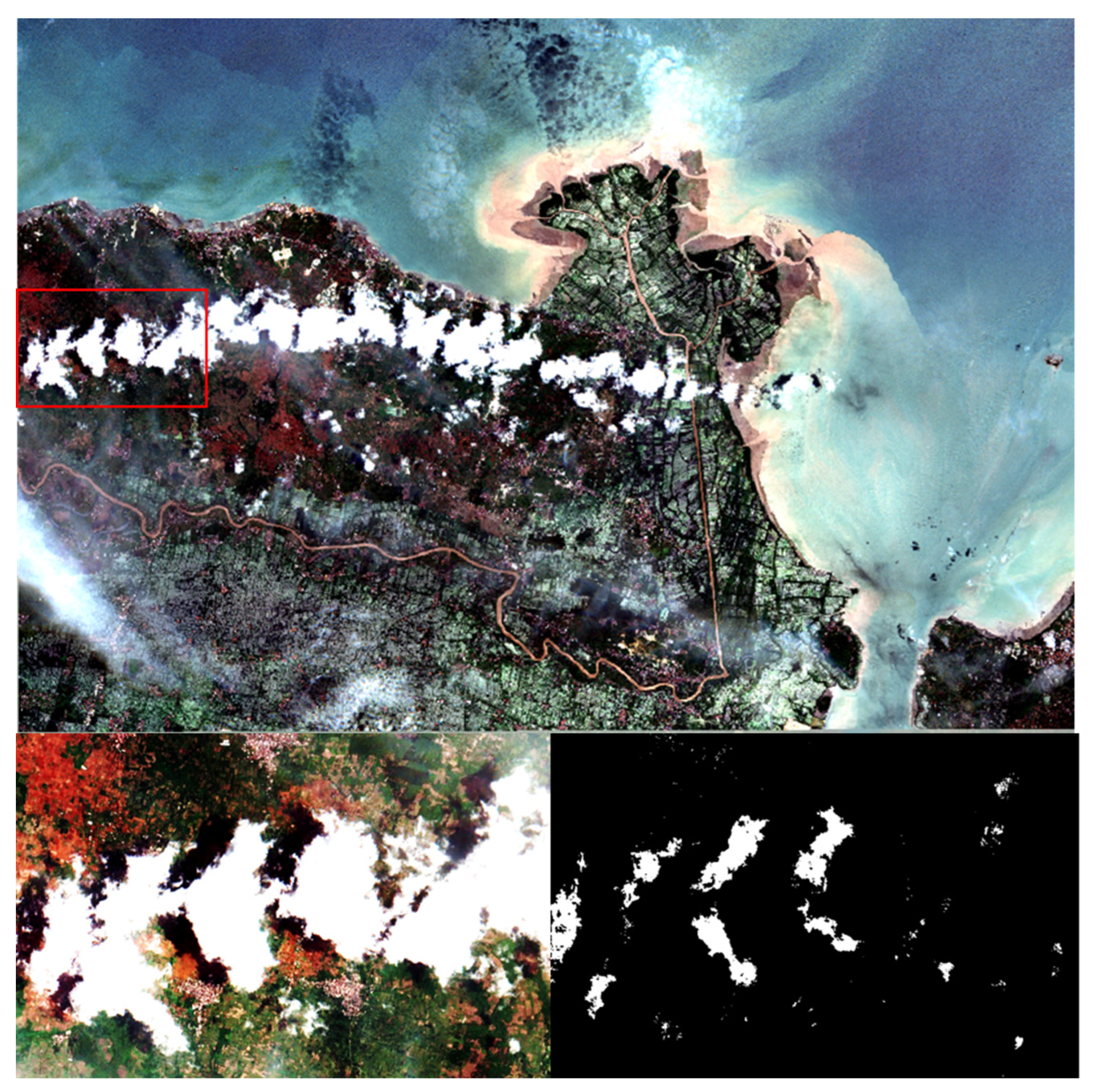
2.1.2. Solo River Mouth, Indonesia

In 2020 it was reported that the Solo River in East Java, Indonesia, was polluted by plastic waste. In the dry season, rubbish covers the surface of the river, making it difficult for fishers to go to sea, while in the rainy season, trash drifts into the sea until it ends up on the beaches in Bali [30].

2.1.3. Srinagar Landfill, India

In 2021, the overflowing landfill site in Srinagar, the capital of Indian-administered Kashmir, was reported to pose a health risk to residents and damage the region’s fragile ecosystem [31].

2.1.4. Tyre Graveyard, Kuwait

Tens of millions of tyres have been held in pits within a graveyard in the Arhiya area, five kilometres south of the city of Jahra [32]. There have been several fires, posing both an environmental and health hazard, so in 2021 the Kuwait government started recycling them.

2.1.5. Almería Greenhouses, Spain

The economy of Almería is dependent on agricultural products, with greenhouses constructed from plastic sheeting producing tons of fruits and vegetables alongside plastic waste. Polyethylene is preferred because of its affordability, flexibility, and ease of manufacturing [33], with the plastics being transparent or translucent with vegetation below. Several papers have focused on detecting the greenhouses themselves, e.g., [34,35,36], while this paper also focuses on the plastic waste between the greenhouses and in abandoned areas.

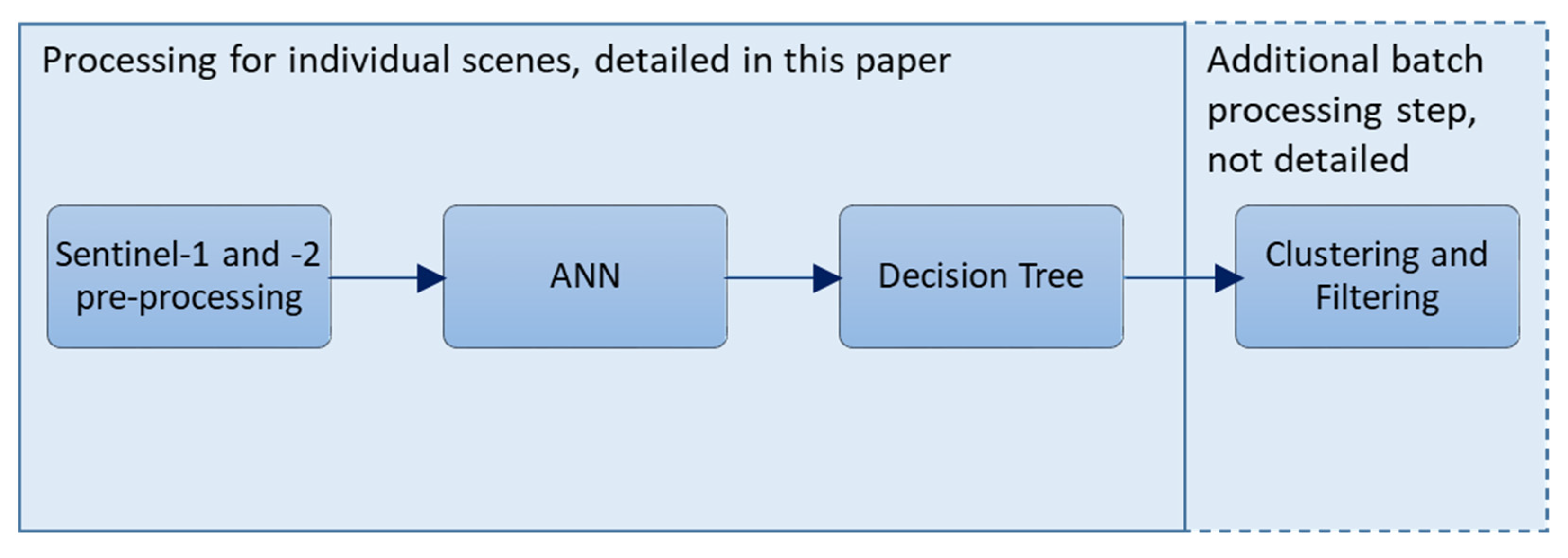
2.2. Classifier Development

All Sentinel files were downloaded through the Copernicus Open Access Hub (https://scihub.copernicus.eu/ (accessed between 2020 and 2022)) and processed using the European Space Agency’s (ESA) open-source Sentinel Application Platform (SNAP) [37] version 7.0.

2.2.1. Pre-Processing

Sentinel-1 Level-1 IW GRDH vertical single polarisation (VV) polarized data were converted to backscatter values using SNAP through: (i) the application of an orbit file to correct for orbital error; (ii) radiometric correction using a Gamma0 coefficient calibration; (iii) Range-Doppler terrain correction through orthorectification against Shuttle Radar Topography Mission (SRTM) 1-arc-second Digital Elevation Model (DEM) data; (iv) the application of a Lee Sigma speckle filter; and (v) conversion to decibels (dB) to produce a non-linear valued output. This workflow is a modified version of the standard SNAP pre-processing workflow to determine the radar backscatter in dB [38], but the thermal noise correction was dropped as it was found to introduce artefacts and is primarily of use for the cross-polarisation channel. The Lee Sigma filtering was included to reduce the speckle while preserving edges [39]. The VV rather than cross-polarisation (VH) data were chosen because they are more sensitive to rough surface scattering [40], and their primary role in the classification process is the separation of water from land.

Sentinel-2 Level-2A data produced by ESA were used to provide bottom-of-atmosphere reflectance imagery. When Level-2A data were unavailable, Level-1C products were atmospherically corrected through the Sen2Cor v2.10 processor [41] available in SNAP.

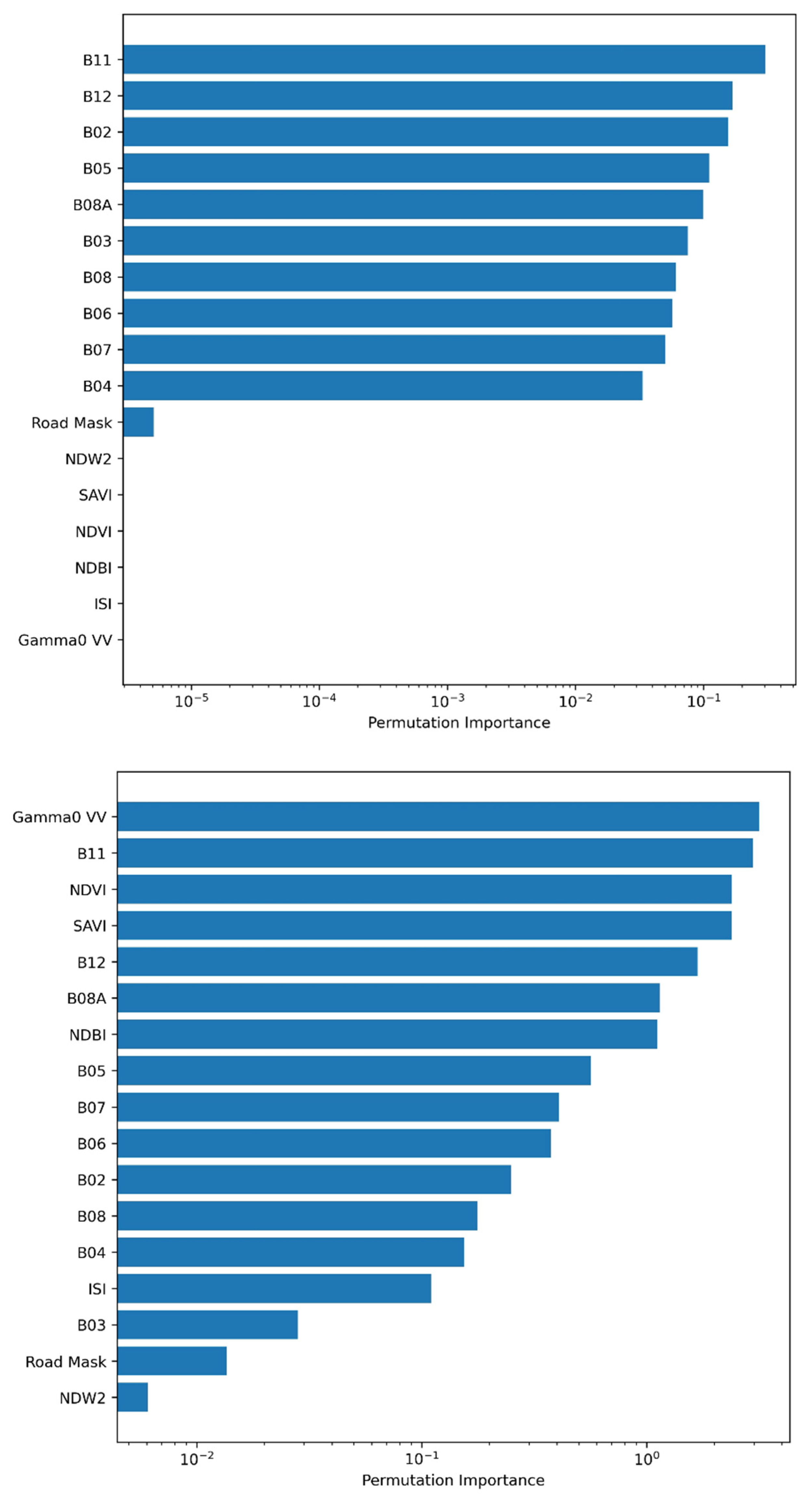
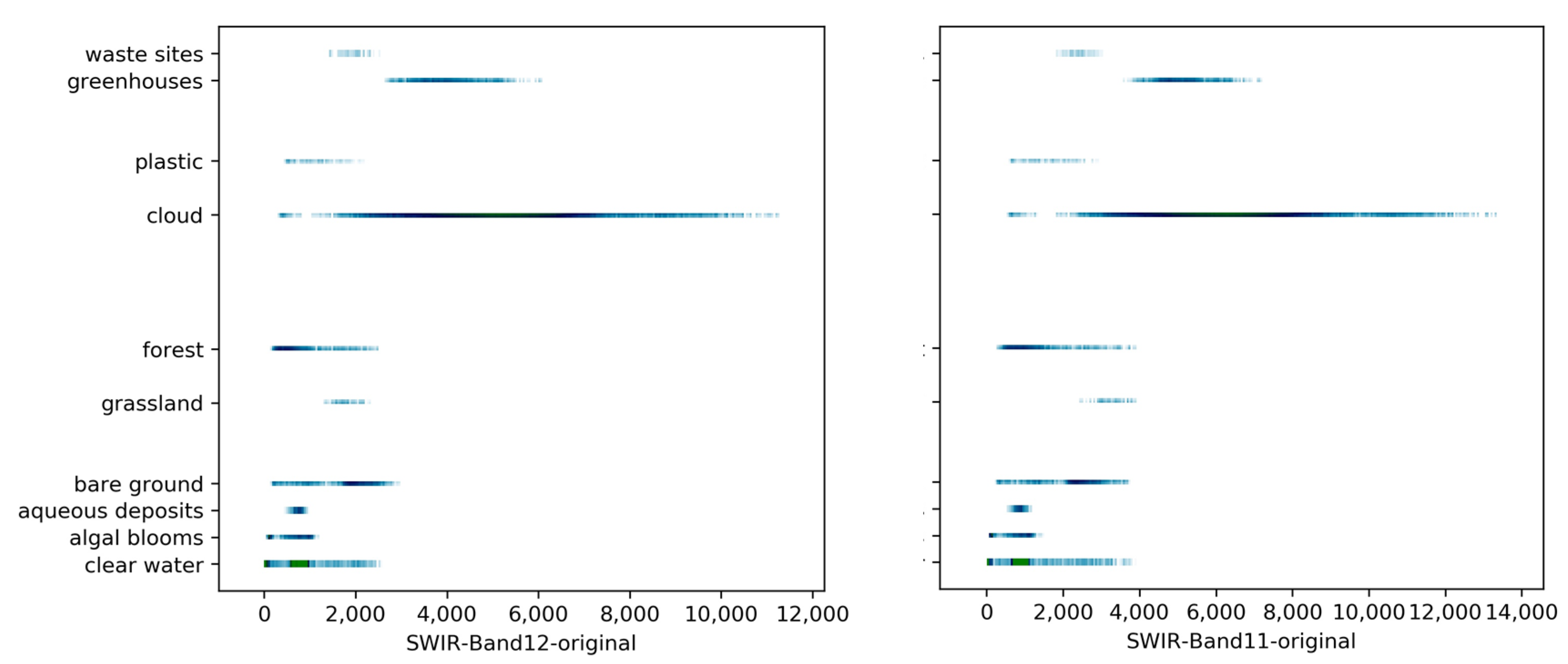
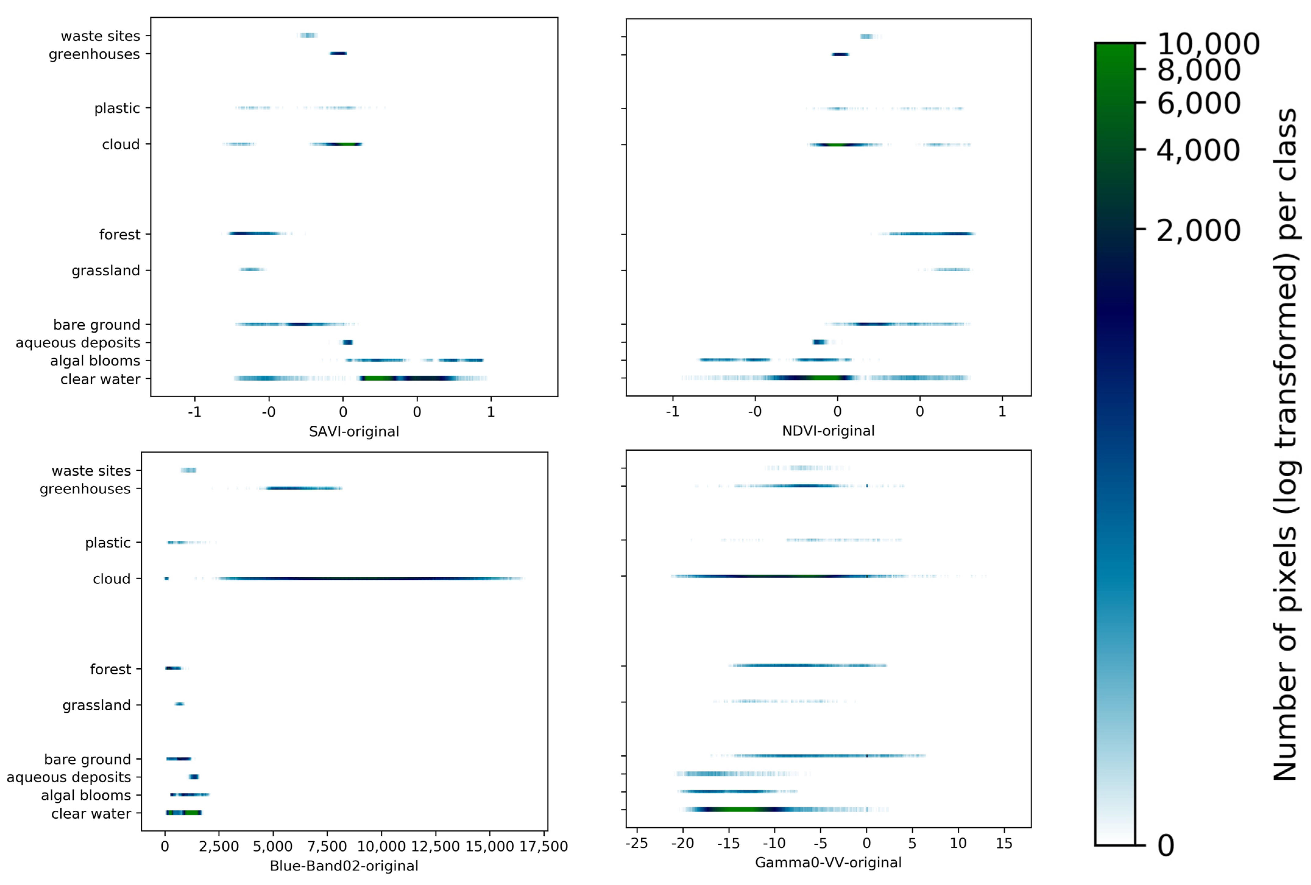
2.2.2. Thematic Indices

A range of optical indices were calculated covering vegetation, biophysical, water and soil thematic groups to aid in the differentiation between land cover types and waste products. The setup started with those used in Page et al. [22] and was adjusted to include additional indices to support the detection of marine plastics alongside waste sites on land.

The normalized difference vegetation index (NDVI) algorithm is a measurement of photosynthetic activity and is strongly correlated with vegetation density and vitality [42]. Designed by Tucker [43], it is based on a high reflectance in the NIR by plant matter in contrast to the strong absorption by chlorophyll-a in the red wavelengths, known as the red edge. For the Sentinel-2 MultiSpectral Instrument (MSI) the chosen bands were band 8 (B08) for the NIR and band 4 (B04) for Red.

$$\mathrm{NDVI}=\frac{\left(\mathrm{NIR}-\mathrm{Red}\right)}{\left(\mathrm{NIR}+\mathrm{Red}\right)}$$

(1)

The soil adjusted vegetation index (SAVI) provides a hybrid between ratio-based and perpendicular indices. It is based on simple radiative transfer and a more coherent theoretical background than other vegetation indices. Developed by Huete [42], it is necessary to use a correction value that varies from 0 for very high vegetation cover to 1 for very low. For use across various land cover types, an intermediate correction value (L) of 0.5 has been used in this instance.

$$\mathrm{SAVI}=\left(1\ast \mathrm{L}\right)\frac{\left(\mathrm{NIR}-\mathrm{Red}\right)}{\left(\mathrm{NIR}+\mathrm{Red}+\mathrm{L}\right)}$$

(2)

The second normalized difference water index (NDWI2) was developed by McFeeters [44] to detect surface waters in wetlands and to allow the measurement of the extent of surface water. The index has reduced errors in separating tyres and plastic from water-dominated pixels. Previous work demonstrated more consistent values for all target land cover classes for NDWI2 compared to its predecessor, NDWI [22], MSI band 3 (B03) was used for Green.

$$\mathrm{NDWI}2=\frac{\left(\mathrm{Green}-\mathrm{Red}\right)}{\left(\mathrm{Green}+\mathrm{Red}\right)}$$

(3)

The Road Mask is based on the approach defined by Fisser [45], which includes the following criteria:

• Visible bands (B02, B03 and B04) > 0.04 to avoid building shadows
• Green/Red ratio (B03/B04) < 0.15 to avoid industry, greenhouses and other surfaces of very high reflectance
• Blue (B02) < 0.4 to be less strict with blue as we target it
• NDVI < 0.7 to avoid vegetation but keep in mind mixed pixels
• NDWI < 0.001 to avoid water [for this work NDWI2 was used
• Normalised Difference Snow Index (NDSI) < 0.0001 to avoid snow
• 0.05 > SWIR (B11) < 0.55

The Normalised Difference Build-Up Index (NDBI) developed by Zha et al. [46] was initially applied to Landsat Thematic Mapper imagery, with MSI B11 used as the SWIR band.

$$\mathrm{NDBI}=\frac{\left(\mathrm{SWIR}-\mathrm{NIR}\right)}{\left(\mathrm{SWIR}+\mathrm{NIR}\right)}$$

(4)

2.2.3. Improved Shadow Masking

Zhou et al. [47] implemented an approach, see Equation (5), to mask cloud shadows in WorldView-3 data in an urban context using the red, green and blue bands. The algorithm was applied to MSI by using the B04, B03 and B02 bands that were first converted into the YCbCr colour space and then the Improved Shadow Index (ISI) was calculated.

$$\mathrm{ISI}=\frac{\mathrm{SI}+\left(1-\mathrm{NIR}\right)}{\mathrm{SI}+\left(1+\mathrm{NIR}\right)}$$

(5)

$$\mathrm{SI}=\frac{\mathrm{Cb}-\mathrm{Y}}{\mathrm{Cb}+\mathrm{Y}}$$

(6)

where Y is the luma component and Cb is the blue-difference chroma component of the Tsai [48] YCbCr model.

To further support the application in aquatic and terrestrial environments as opposed to the original purely urban context, the resulting ISI layer was adjusted using NDWI2; otherwise, all open water pixels were flagged as shadow—as a result, the shadow mask is not triggered over water, but this was not foreseen as an issue as the miss-classification of plastic due to shadow is not an issue encountered over water. Additionally, to account for terrain shadowing, which can also cause misclassification, the terrain slope was calculated from the DEM, SRTM accessed during the Sentinel-1 processing, and high slope pixels were added to the ISI to create a raster layer termed the shadow mask. Figure 1 shows an example of the developed shadow mask applied to an area with clouds. The ISI was used as a layer in the ANN, while the shadow mask was used in the post-processing decision tree that reassigns pixels that the ANN has misclassified.

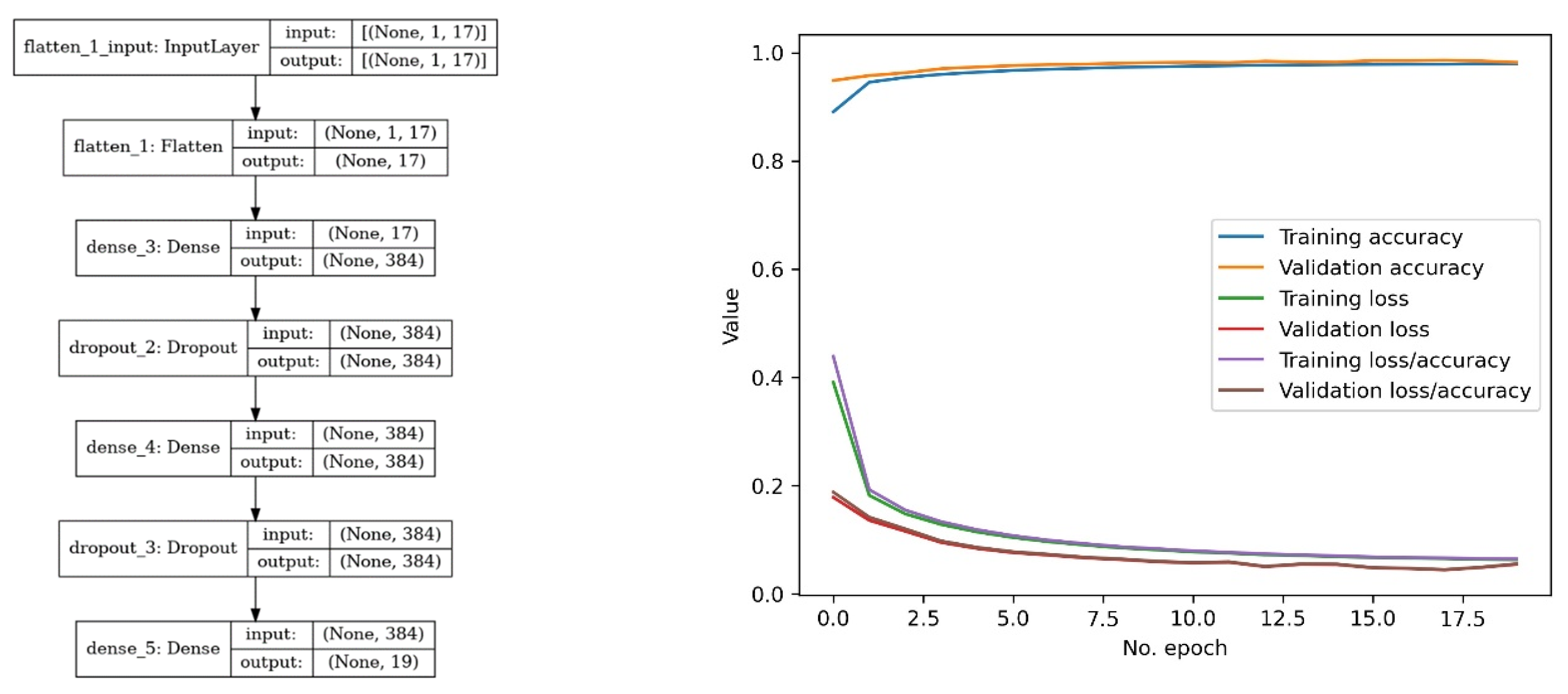
2.2.4. Neural Network

ANNs are mathematical models inspired by the structure and behaviour of the human brain. The multilayer perceptron supervised learning approach has multiple layers with the information transferred from the input layer to the output (feed-forward), and the weights are changed until the simulated outputs are similar to the observed ones [49].

All thematic indices were stacked into one file alongside a subset of Sentinel-2 MSI bands, and the Sentinel-1 Gamma0 VV data. The resulting stack consists of 17 layers (

Table 2. Layers within the classification stack, including the spatial resolution and MultiSpectral Instrument (MSI) band and central wavelength for the Sentinel-2 reflectance bands.

Layer Number	MSI Band Number and Central Wavelength (nm)	Description	Original Spatial Resolution (m)
1	B02 (490)	Blue	10
2	B03 (560)	Green	10
3	B04 (665)	Red	10
4	B05 (705)	Red Edge	20
5	B06 (740)	Red Edge	20
6	B07 (783)	Red Edge	20
7	B08 (842)	NIR	10
8	B08A (865)	Red Edge	20
9	B11 (1610)	SWIR	20
10	B12 (1190)	SWIR	20
11		NDVI	10
12		SAVI	10
13		NDWI2	10
14		Road Mask	10
15		NDBI	10
16		ISI	10
17		Gamma0 VV	5 × 20

). Different Sentinel-2 bands have different spatial resolutions in the original Sentinel datasets, so the coarser spatial resolution band were resampled to 10 m. For Sentinel-2, this occurs just before inclusion in the stack using the SNAP raster resampling tool, and for Sentinel-1 it is included as part of the terrain correction.

An augmented land cover classification is the desired output of the ANN classifier, which is separated into nine classes (see

Table 3. Classification of the land cover types through a tiered approach following CORINE, with an additional Level 2 class for plastics.

Level 1		Level 2		Level 3
1.	Water	1.1.	Clear Water
		1.2.	Algal Blooms
		1.3.	Aqueous Deposits
2.	Land	2.1.	Non-Photosynthetic
		2.2.	Green Vegetation	2.2.1.	Woodland
				2.2.2.	Grassland
		2.3.	Urban	2.3.1.	Industrial
				2.3.2.	Artificial Surfaces
		2.4.	Plastics	2.4.1	Tyres
				2.4.2	Plastic
				2.4.3	Greenhouses
				2.4.4	Waste sites

). These classes are adapted from the CORINE land cover mapping scheme [50], a consistent classification system developed for application in Europe. The classes were modified by adding plastics as an additional Level 2 class and then the different types of plastics (where plural the paper refers to the four Level 3 classes together).

The training/validation dataset used Sentinel-1 and -2 satellite imagery collected over a global set of 30 test sites; see Figure 2. Test sites were accumulated over several years by reviewing peer-reviewed papers, reports and news articles on plastic waste and its detection using remote sensing. Training pixels manually identified using a combination of the high spatial resolution satellite imagery within Google Earth and the Sentinel-2 RGB colour composite. Where the locations of the plastics could not be reliably identified, these land cover classes were not digitized, and the background land cover classes were only digitized so as not to reduce the accuracy of the overall dataset.

For each target class, multiple homogeneous training pixels were taken across the different sites through the digitizing of polygons. Figure 3 shows the digitization for the Višegrad Dam aquatic site and tyre graveyard in Kuwait with the digitized pixels shown as crosses overlaid on the Sentinel-2 pseudo-true colour (left) and SAR backscatter image shown on the right. The fusion of Sentinel-1 and -2 for land cover mapping provides the land surface’s combined spectral and structural characteristics, with the results often having a higher accuracy than using either of the datasets individually [51]. For the Višegrad Dam, the SAR image shows that the floating mass has a higher backscatter than the water before the dam accumulation (top right), and similarly the tyre graveyard also shows higher backscatter for the filled tyre pits compared to the surrounding sand and empty pits (bottom right).

The top 25 sites in

Table A1. Full training/validation dataset in alphabetical order with Sentinel-1 IW GRDH and Sentinel-2 Level 2A files as date/time and (for Sentinel-2) tile.

Test Site	Sentinel-1 IW GRDH	Sentinel-2 L2A
Alexandrov Landfill, Russia	S1B 20200928T033648 S1B 20210502T033646	S2B 20200923T083659 T37VDC S2B 20210511T083559 T37VDC
Almería Greenhouses, Spain	S1A 20210408T061050	S2A 20210505T105031 T30SWF
Chemor Landfill, Malaysia	S1A 20180901T230325	S2A 20181026T032821 T47NQF
Dandora Landfill, Kenya	S1A 20200209T155606	S2B 20200208T074009 T37MBU
Empang River Mouth, Indonesia	S1A 20210225T111520	S2B 20210228T025649 T48MXU
Gioto Landfill, Kenya	S1A 20210603T155640	S2A 20210610T074611 T36MZE
Jakata Landfill, West Java	S1A 20190819T223351	S2B 20190818T025549 T48MYU
Jenjarom, Malaysia	S1A 20190424T225548	S2A 20190424T032541 T47NQD
Kerala Landfill, India	S1A 20210314T004059	S2A 20210314T050651 T43PFM
Kuta Beach, Bali	S1A 20190216T104117	S2B 20190217T021749 T50LKR
Madrid Landfill, Spain	S1A 20211115T061821	S2A 20211114T110321 T30TVK
Manilla, Philippines	S1A 20170313T214633	S2A 20170314T023321 T51PTS
Mucar Port, Java	S1A 20190727T104933	S2A 20190725T022551 T49LHL
PML beach target, England [57]	S1B 20180515T063101	S2B 20180515T112109 T30UVA
Scotland, various sites used for Page et al. [21]	S1B 20180625T063732	S2B 20180627T113319 T30VVH
Serayu River Mouth, Indonesia	S1A 20200613T110629	S2B 20200610T024549 T49MBM
Seyhan, Turkey	S1A 20211210T034252	S2B 20211211T082239 T36SXG
Solo River Mouth, Indonesia	S1A 20210218T220906 & 20210218T220931 **	S2A 20210227T023641 T49MFN
Srinagar Landfill, India	S1A 20211031T005910	S2A 20211029T053941 T43SDT
Tapuhia Landfill, Tonga	S1A 20220220T061455	S2B 20220216T215909 T01KFS
TPA Kabupaten Tangerang, Indonesia [65]	S1A 20210422T223357	S2A 20210424T025541 T48MXU
Landfill, Turkey	S1A 20211026T040642	S2A 20211026T085041 T35TPE
Tyre Graveyard, Kuwait	S1A 20201228T024734 & 20201228T024709 **	S2A 20201226T073321 T38RQT
Višegrad Dam, Bosnia-Herzegovina	S1A 20210302T163318	S2A 20210302T09303 T34TCP *
Walleys Landfill, England	S1B 20200920T062219	S2B 20200921T112119 T30UWD
Additional sites used only for the accuracy assessment
Accra, Ghana	S1A 20220130T181813	S2B 20220126T102209 T30NYM
Ankara Tyre Site, Turkey	S1A 20211027T155127	S2B 20211028T083949 T36TVK
Hamburg, Germany	S1A 20220326T053329	S2A 20220325T102651 T32UNE
Mariupol, Ukraine	S1A 20220111T152022	S2A 20220108T083331 T37TCN
Windrow, Haiti	S1A 20201220T230129	S2B 20201222T153619 T18QYF

* Processed from Level 1C to Level 2A as there were issues using the online Level 2 file. ** Two Sentinel-1 files merged to cover the area of interest for the test site fully.

were used for training/validation, which resulted in the pixel numbers shown in

Table 4. Training sample distribution amongst the classes.

Class	Original Number of Pixels	Original Percentage	Updated Number of Pixels	Updated Percentage
Clear Water	810,210	65.4%	587,792	47.5%
Algal Blooms	10,184	0.8%	27,773	2.2%
Aqueous Deposits	37,924	3.1%	47,191	3.8%
Bare Ground	34,307	2.8%	44,659	3.6%
Murrum Soil	56	0.0%	20,683	1.7%
Sand	9097	0.7%	27,012	2.2%
Grassland	11,513	0.9%	28,703	2.3%
Shrubland	10,341	0.8%	27,882	2.3%
Forest	31,502	2.5%	42,695	3.4%
Cropland	7939	0.6%	26,201	2.1%
Buildings	7038	0.6%	25,570	2.1%
Artificial Surfaces	7519	0.6%	25,907	2.1%
Cloud	247,323	20.0%	193,771	15.6%
Shadow	7387	0.6%	25,815	2.1%
Plastic	667	0.0%	21,111	1.7%
Tyres	351	0.0%	20,889	1.7%
Greenhouses	4163	0.3%	23,558	1.9%
Waste Sites	1143	0.1%	21,444	1.7%
Total number after adjustment	1,238,656 pixels split into 928,992 training pixels and 309,664 validation pixels

. As the original plastics classes of interest have low numbers of pixels, such that they are from 0% to 0.3% of the total pixels to within 1dp, the training/validation dataset has a class imbalance. Therefore, a re-weighting was applied to reduce the number of pixels for the classes with high numbers, such as clear water and clouds, and increased the number of pixels for classes with low numbers through duplication. The decision on which classes had their values decreased versus increased was based on their original percentages; greater or less than 5.6% that equated to the total number of pixels divided by the number of classes. The result is that this approach has reduced the class imbalance, although it remains and should be accounted for when assessing performance.

Different models were tested to investigate the bands that could be used and their relative contribution: Linear Regression, Random Forest and ANN. As it was difficult to understand the different input layer contributions to the ANN output, the relative importance was tested using the two other types of models. Figure 4 shows the resulting layer importance graphs for applying Linear Regression (top) and Random Forest (bottom) models generated using the permutation importance function in the sklearn Python module; it was not possible to apply this function to the ANN due to its model structure that was not compatible. The graphs are log-scaled as the single bands for the Linear Regression model contribute significantly more than the SAR-derived roughness. In contrast, all layers except for the Road Mask significantly contribute to the Random Forest model.

The ANN model, shown in Figure 5 (left), was generated using a Sequential model that creates a deep learning model by adding layers; sequential patterns are important because they can be exploited to improve the prediction accuracy of classifiers. The layers include:

• Flatten is used to flatten all its input into a single dimension.
• Dense implements a regular, deeply connected neural network layer that receives inputs from all neurons in the previous layer and applies a matrix-vector multiplication.
• Dropout reduces the training dataset size so that overtraining does not occur.

The model training used the KerasTuner [52] to iteratively perform testing until the optimal model setup was achieved in terms of the overall accuracy achieved with the resulting Loss function shown in Figure 5 (right) used to diagnose the behaviour of the model. In this case, as should occur, the training and validation plots of loss and accuracy have converged over successive epochs.

Figure 6 shows the confusion matrices generated during the training to indicate the ANN and RF performance across all land cover classes. For the ANN (Figure 6 top), there is some misclassification, but overall, most validation pixels fall on the prime diagonal; a value of 1.0 indicates all validation pixels were assigned to the same class they were digitized according to. A similar result is seen for the Random Forest model (Figure 6 bottom) but with increased confusion between bare ground and tyres.

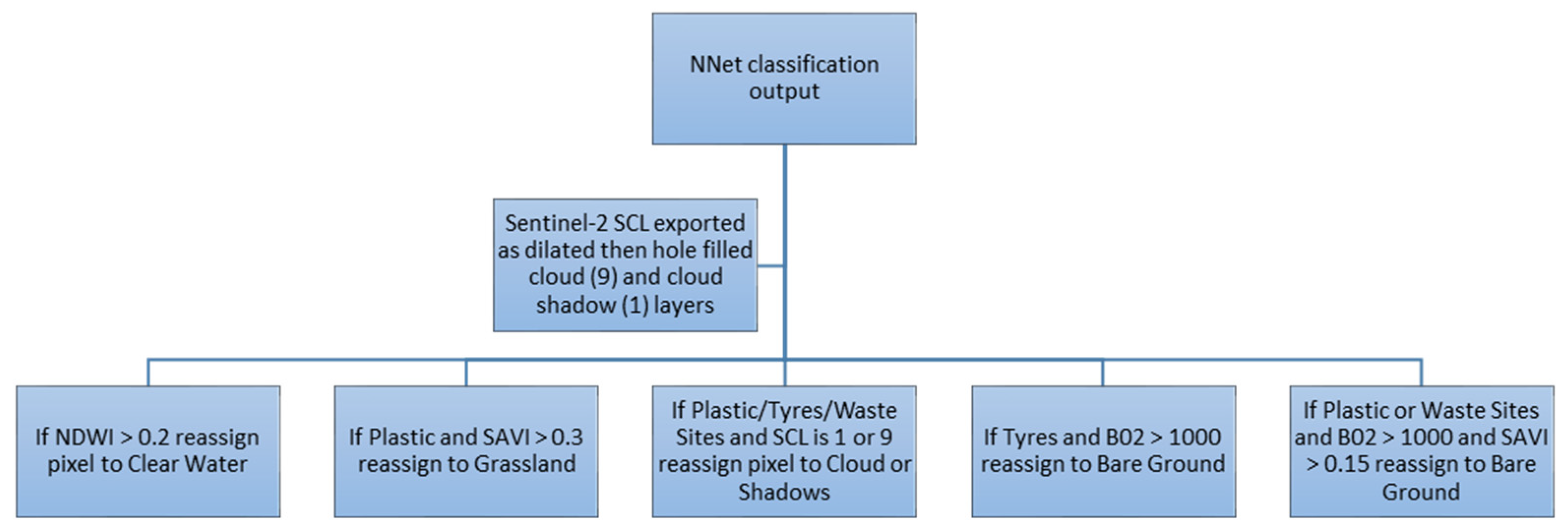
2.2.5. Post Neural Network Decision Tree

The post-ANN decision tree, see Figure 7, was used for reclassification. It was discovered through testing the performance across multiple sites that the ANN could not fully capture a radiometric interpretation of the surface and is also not designed to accept categorical layers.

The Sentinel-2 Scene Classification Layer (SCL) was extracted from the Sentinel-2 L2A file and resampled to 10 m resolution; pixels classified as cloud (value of 9) and cloud shadow (value of 1) were used. Then, the Python multidimensional image processing library (scipy.ndimage) was then applied so the pixel values were extracted as dilated and hole-filled binary layers. This meant that both cloud edges and cloud shadow edges could be captured, which was essential as both can end up misclassified as plastics. Additionally, the previously calculated shadow mask (Section 2.2.3) was used to further exclude pixels influenced by shadow from being classified as plastics and plastic/tyre/waste pixels were reclassified where they had a high NDWI2 value, high SAVI value or high B02 reflectance, as these were found to be frequent misclassifications.

Figure 8 shows the classification results’ differences before (top) and after (bottom) the post-network decision tree. The cloud shadows (grey) have been filled in as the pixels within these are likely to be incorrect. In addition, the number of plastic (red) pixels have been reduced in the top right to what mixed cloud pixels exist. Incorrectly, bare ground cultivated pixels are classified as waste sites (lilac) as the current bare ground training data are not sufficiently capturing the soil’s spectral properties. In the RGB pseudo-true colour composite (Figure 1), the soil appears red, which might alternatively indicate the atmospheric correction is erroneous due to the high aerosol load.

2.3. Accuracy Assessment Methodology

The correctness of a classification can be evaluated by computing the number of correctly recognized class examples (True Positives, TP), the number of correctly recognized examples that do not belong to the class (True Negatives), and examples that either were incorrectly assigned to the class (False Positives, FP) or that were not recognized as class examples (False Negatives, FN) [53]. These four counts constitute a confusion matrix, from which Precision and Recall are calculated and commonly used to evaluate classification performance [54]:

$$\mathrm{Precision}=\frac{\mathrm{TP}}{\left(\mathrm{TP}+\mathrm{FP}\right)}$$

(7)

$$\mathrm{Recall}=\frac{\mathrm{TP}}{\left(\mathrm{TP}+\mathrm{FN}\right)}$$

(8)

Precision (Equation (7)) quantifies the proportion of the predicted positives that were truly positive, while Recall (Equation (8)) is a measure of the proportion of actual positives which were classified correctly. The average of all accuracy values yielded the aggregate average Precision.

As accuracy is not a good metric to use when there is a class imbalance, which we have, the F1-score that assesses the Precision-Recall trade-off has also been calculated [54]; see Equation (9). The F1-score ranges from zero to one, with a high value indicating high classification performance.

$$\mathrm{F}1-\mathrm{score}=\frac{2\ast \mathrm{Precision}\ast \mathrm{Recall}}{\mathrm{Precision}+\mathrm{Recall}}$$

(9)

Additionally, Cohen’s KAPPA coefficient is a statistical measure of agreement that provides a more robust result than percentage agreement calculations [55]. In the equations below, p_o is the observed agreement (percentage of instances classified correctly from the error matrix), and p_e is the expected agreement. The overall expected agreement is calculated using Equation (10), where the expected agreement is calculated for each class, and then these are added together and divided by the total number of pixels.

$$\mathrm{KAPPA}=\frac{\left({\mathrm{p}}_{\mathrm{o}}-{\mathrm{p}}_{\mathrm{e}}\right)}{\left(1+{\mathrm{p}}_{\mathrm{e}}\right)}$$

(10)

$${\mathrm{p}}_{\mathrm{e}}=\frac{\left({\mathrm{expected}}_{\mathrm{class}1}+{\mathrm{expected}}_{\mathrm{class}2}+\dots \right)}{\mathrm{N}}$$

(11)

$${\mathrm{expected}}_{\mathrm{class}1}=\frac{\left({\mathrm{actual}}_{\mathrm{class}1}{\ast \mathrm{estimated}}_{\mathrm{class}1}\right)}{\mathrm{N}}$$

(12)

3. Results

This section showcases the effect of the decision tree, accuracy statistics extracted during the training process and the classification results for the Test sites.

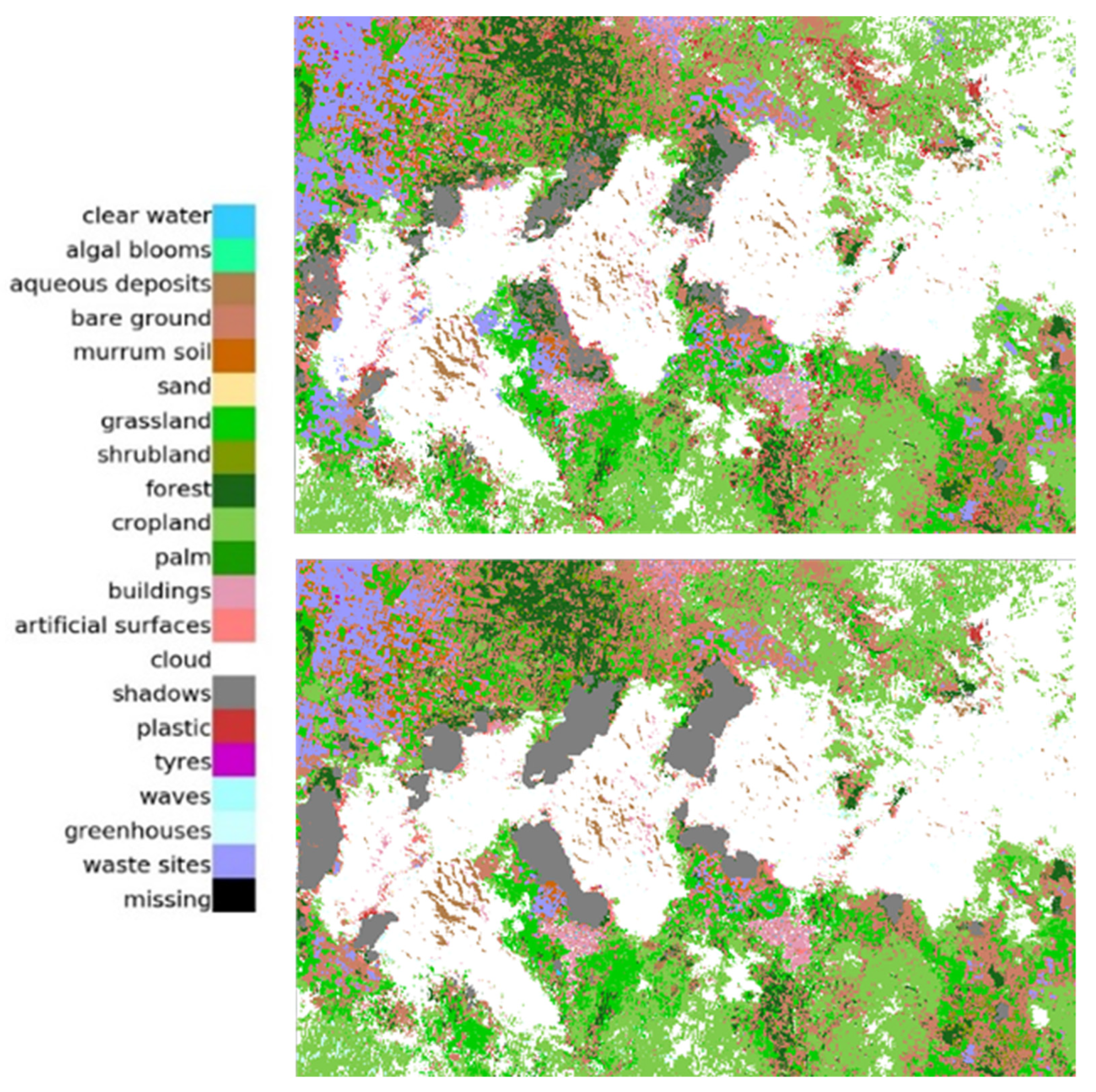
3.1. Decision Tree Impact

Figure 8 and Figure 9 shows the impact of the decision tree on the ANN classification output. For Figure 8, the focus of the example is removing spurious plastics pixels that are caused by cloud shadow. In Figure 9, it is the over classification of bright bare ground incorrectly classified as plastic or waste sites. The determination of the thresholds, shown in Figure 7, was based on analysis of the data held in the training/validation dataset so this biases the accuracy towards locations already encountered.

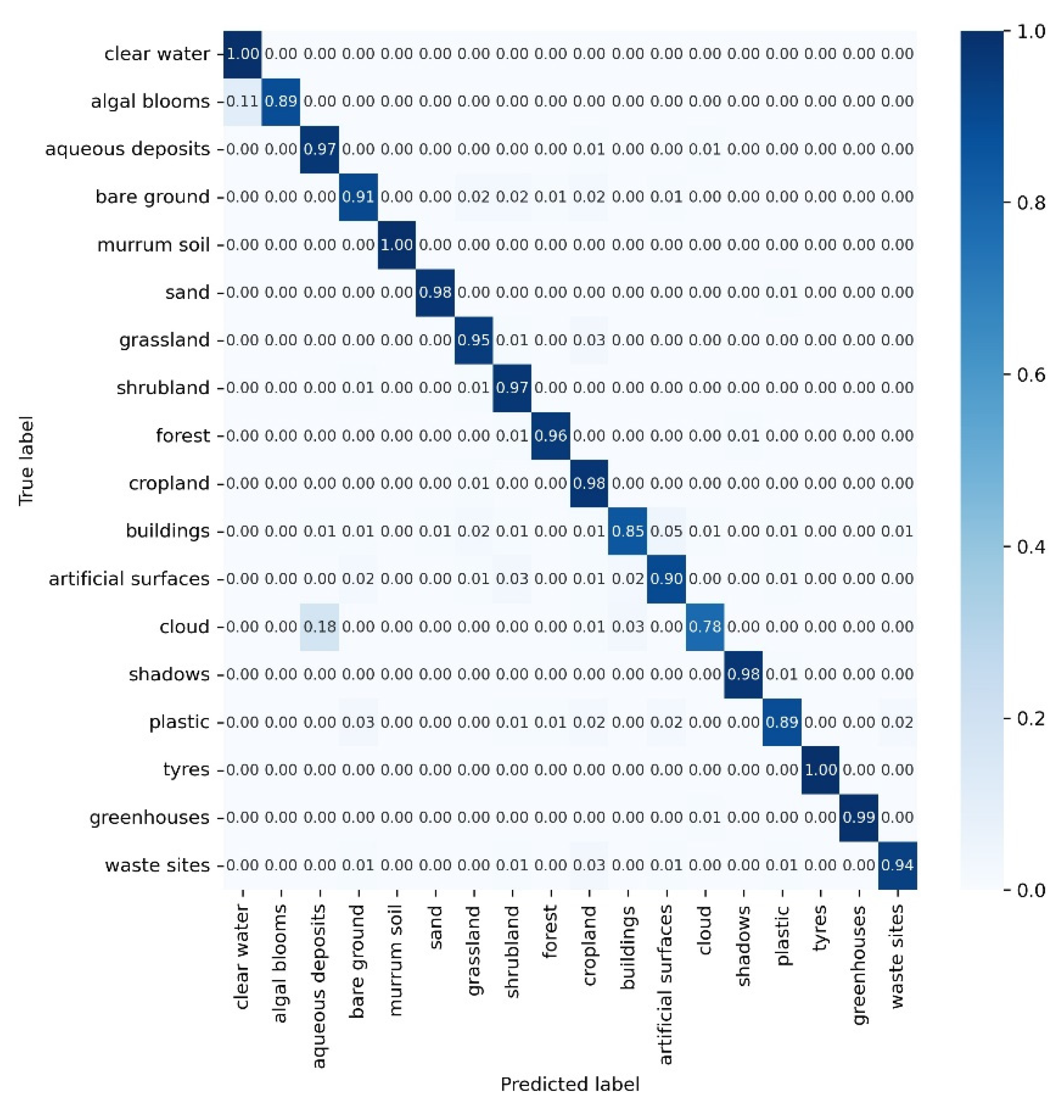
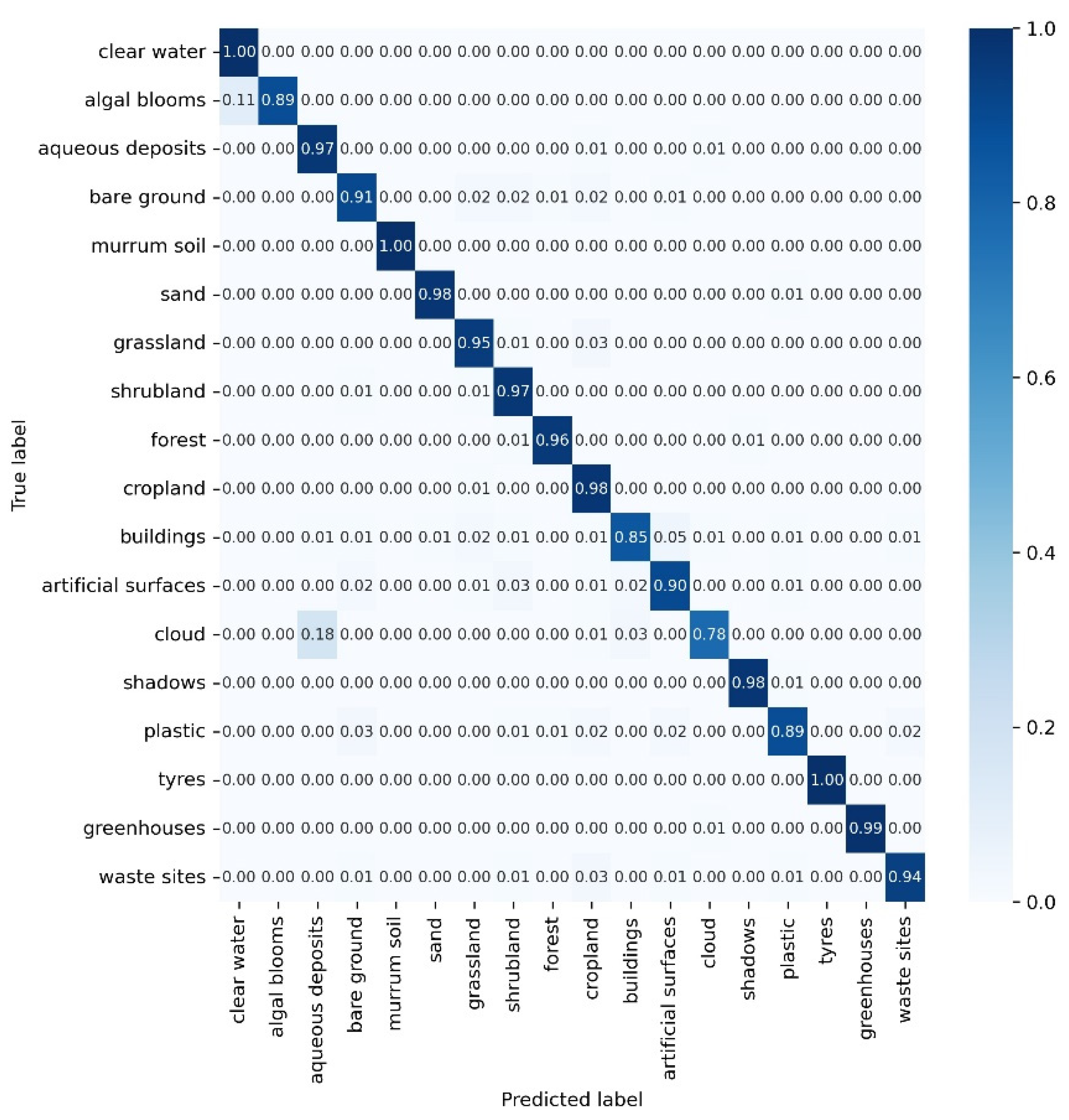
3.2. Accuracy Assessment

The accuracy statistics for the developed classifier are shown in

Table 5. ANN accuracy statistics generated during the training process.

Class	Precision	Recall	F1-Score
Clear Water	0.99	1.00	1.00
Algal Blooms	1.00	0.89	0.94
Aqueous Deposits	0.57	0.89	0.72
Bare Ground	0.95	0.92	0.93
Murrum Soil	1.00	1.00	1.00
Sand	0.99	0.98	0.98
Grassland	0.92	0.95	0.94
Shrubland	0.90	0.97	0.93
Forest	0.96	0.96	0.96
Cropland	0.84	0.98	0.91
Buildings	0.78	0.85	0.82
Artificial Surfaces	0.91	0.90	0.91
Cloud	0.99	0.78	0.88
Shadow	0.99	0.98	0.98
Plastic	0.91	0.90	0.90
Tyres	1.00	1.00	1.00
Greenhouses	0.99	0.99	0.99
Waste Sites	0.95	0.94	0.94
Aggregate average Precision	0.950
KAPPA coefficient	0.860

, with the Precision and Recall alongside F1-score calculated for each class. To improve the robustness of the assessment, an additional five validation sites (shown at the bottom of Table A1) were added that were not included in the iterative model training/validation process and that statistics recalculated; shown in

Table 6. Classifier accuracy statistics after the addition of five validation sites (shown at the bottom of Table A1).

Class	Precision	Recall	F1-Score
Clear Water	0.99	1.00	1.00
Algal Blooms	0.99	0.89	0.94
Aqueous Deposits	0.28	0.97	0.44
Bare Ground	0.97	0.91	0.94
Murrum Soil	0.74	1.00	0.85
Sand	0.99	0.98	0.98
Grassland	0.88	0.95	0.91
Shrubland	0.87	0.97	0.92
Forest	0.95	0.96	0.96
Cropland	0.72	0.98	0.83
Buildings	0.45	0.85	0.59
Artificial Surfaces	0.88	0.90	0.89
Cloud	1.00	0.78	0.88
Shadow	0.96	0.98	0.97
Plastic	0.43	0.89	0.58
Tyres	0.95	1.00	0.97
Greenhouses	0.91	0.99	0.95
Waste Sites	0.74	0.94	0.83
Aggregate average Precision	0.820
KAPPA coefficient	0.897

.

In Table 5, all the Precision values except Aqueous Deposits are high, greater than 0.8, equating to the classifier being correct more than 80% of the time. When the addition validation sites are included, Table 6, all classes remain high (greater than 0.7) except for the Aqueous Deposits, Building and Plastic. These classes have a highly variable spectral shape across the training/validation datasets and so a single class is a generalization of that variability. The Plastic class was strongly influenced by the inclusion of sites such as Haiti with a windrow that was not detected; see Figure 10. The windrow can see be visible seen in the stretched pseudo-colour composite, Figure 10 (bottom left), but is not visible in the unstretched Sentinel-2 pseudo-colour composite or backscatter image.

All the Recall values are also high; the classifier can capture most of the positive predictions. As a result, the F1-scores are high except for those classes with a low Precision, i.e., both Precision and Recall are high. This behaviour is evident in both Table 5 and Table 6, where the classes with low Precision scores have lower F1-scores.

In terms of the overall statistics, the average Precision and KAPPA coefficient were calculated for the aggregate of all the classes, with both also presenting high values of 95% and 0.86 in Table 5. For Table 6, the aggregate Precision has dropped to 0.820 but the KAPPA has increased to 0.897. KAPPA is better at assessing imbalanced class problems, and a value of greater than 0.81 is classified as “Almost Prefect” [56].

Figure 11 shows examples of layer values extracted from the test sites for the Sentinel-2 bands 12 and 11 in the SWIR, SAVI and NDVI vegetation indices, Sentinel-2 band 2 (blue) and the Sentinel-1 Gamma0 VV layers. In terms of importance, these are the top six layers identified when the Random Forest model was executed on the training dataset; see Figure 4 (bottom), and the increased blue darkness followed by green indicates a greater number of pixels as indicated by the legend. For the plastics categories, there is a separation, but the layer pixel ranges do overlap with non-plastic classes. So, for example, greenhouses exist within the range of pixel values seen within clouds.

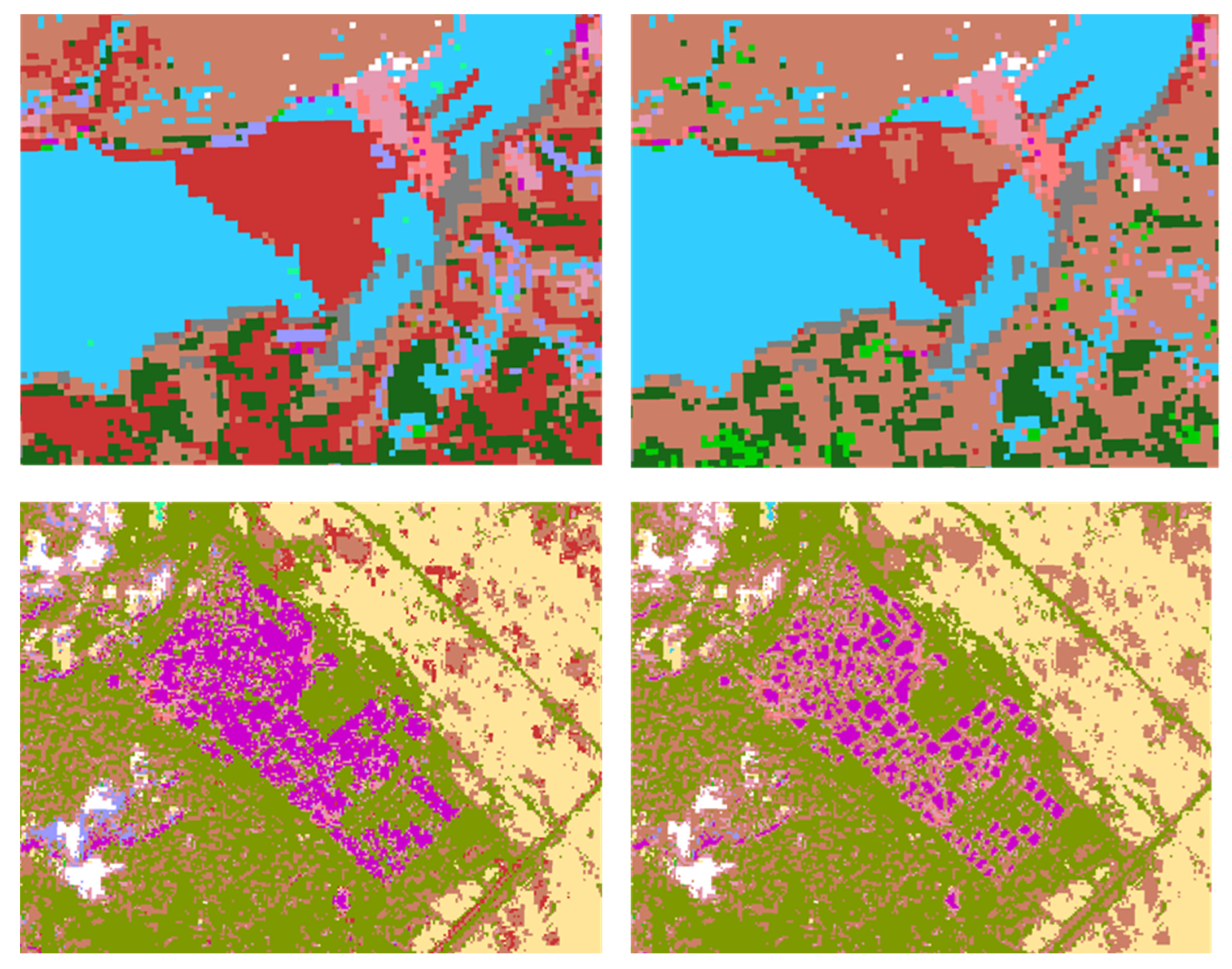
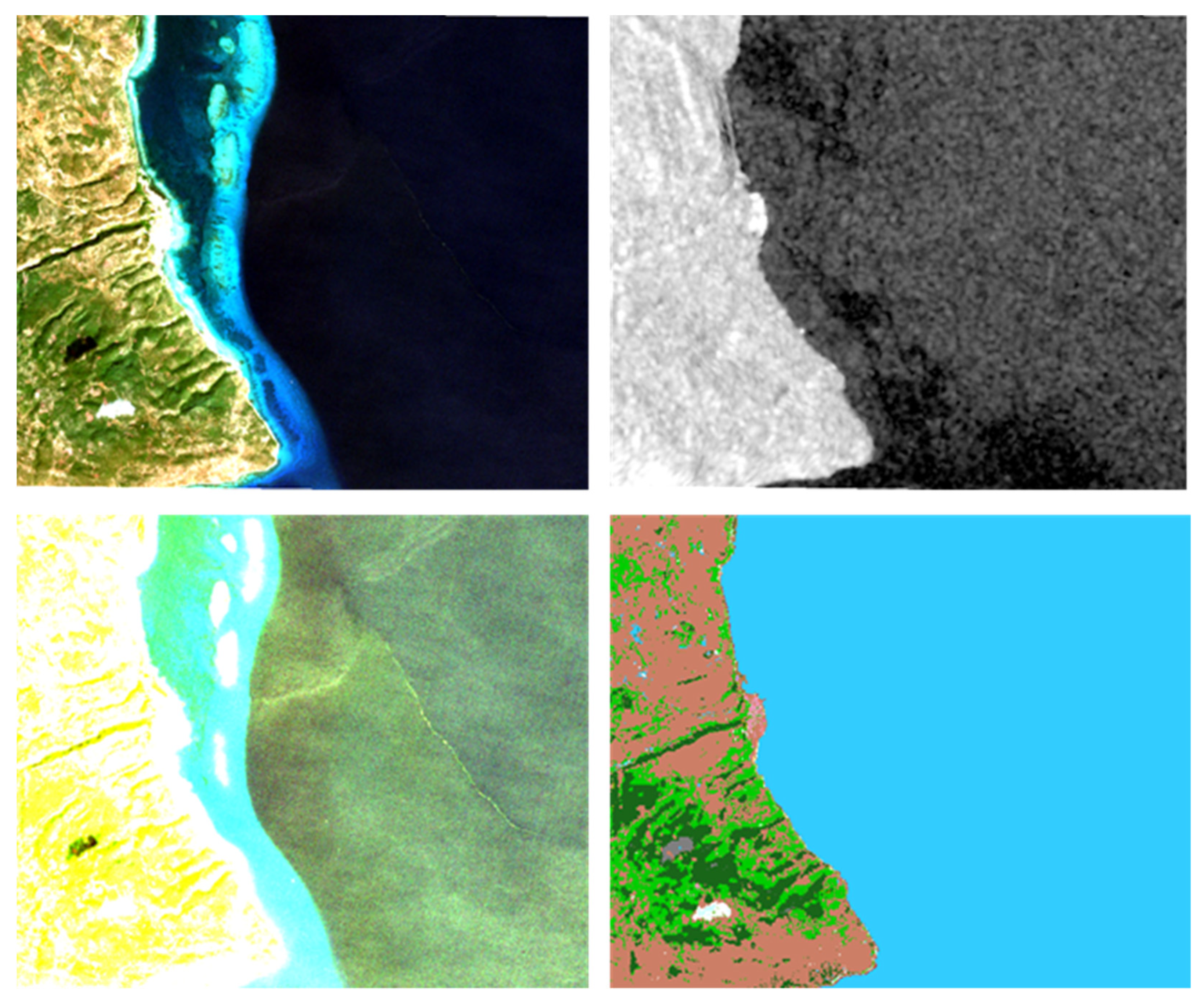
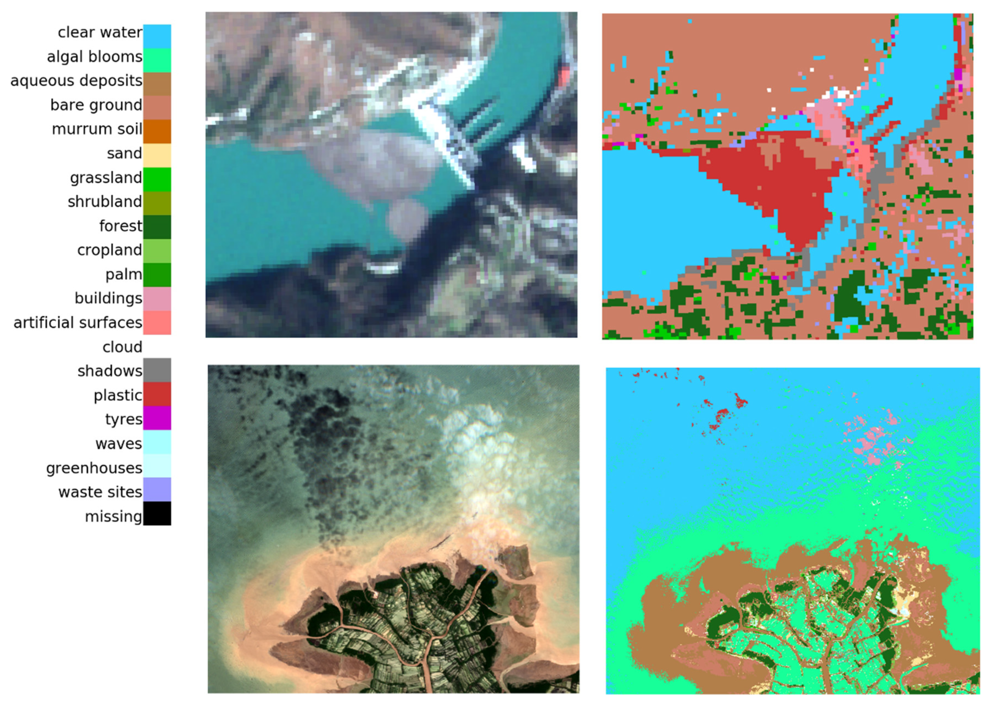
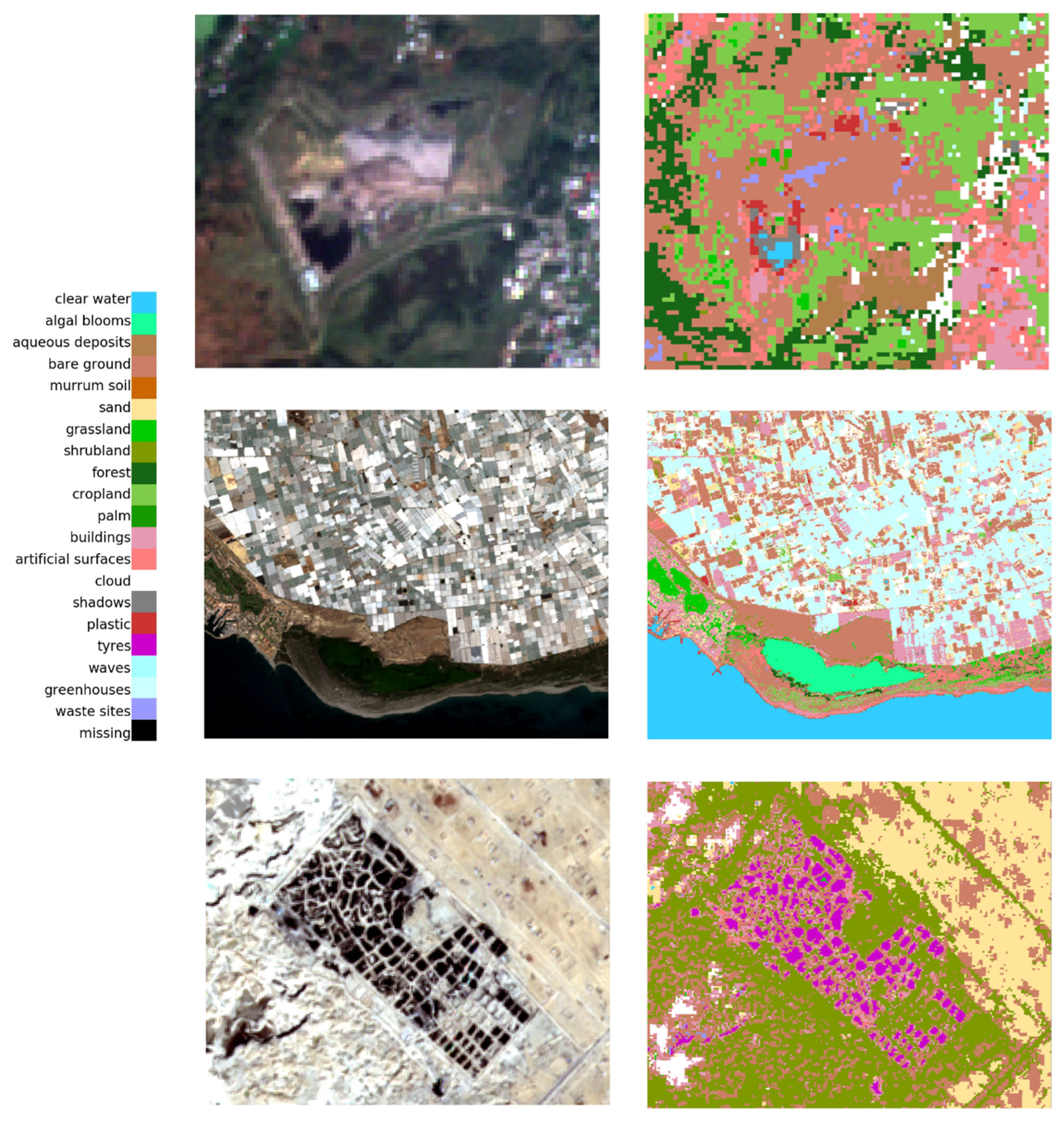
3.3. Application to the Test Sites

Figure 12 and Figure 13 show the results of the classifier applied to the five test sites, which indicates the performance for different types of plastic and with varying land cover backgrounds.

For the Višegrad Dam river accumulation, Figure 12 (top), and Solo mouth test site, Figure 12 (bottom), it is predominately plastic (red) that is being detected. For the river mouth example, there are thin cloud and cloud shadow pixels, and some are classified as artificial surfaces where the cloud masking has not removed all cloud pixels.

A mixture of plastic (red) and waste sites (lilac) pixels are being classified for the Srinagar Landfill in Figure 13 (top). For the Almería province of Spain, on the coast, Figure 13 (middle) shows an area dominated by greenhouses, with the greenhouses themselves being classified according to this category (light blue) but also as clouds (white) and buildings (pale pink). In between the greenhouses, there are areas classified as plastic (red) that coincide with the storage of water within pools lined with black plastic. The third site, Figure 13 (bottom) is the tyre graveyard in Kuwait, with the tyre pits predominately classified correctly (cerise), although there are also pixels classified as artificial surfaces (bright pink).

4. Discussion

The usage of Sentinel-2 for detection plastic waste is the focus of numerous papers as its combination of wavebands and high spatial resolution imagery alongside systematic acquisition provides a dataset not available from other missions. Martínez-Vicente et al. [57] identified a separation between requirements for land/shoreline and in/on water plastic waste due to the higher temporal variability of the processes controlling marine plastic debris floating or in water compared to those controlling marine plastic dynamics on the shore. However, new missions are being developed/launched that can act as an improvement to what Sentinel-2 offers alone. For example, Garaba et al. [58] demonstrated the potential of high spatial and spectral resolution AVIRIS airborne imagery of a landfill and its neighbouring industrial and water treatment facilities. Additionally, Taggio et al. [59] have combined ML with pan-sharpened hyperspectral satellite data from the recently launched, 2019, PRecursore IperSpettrale della Missione Applicativa (PRISMA) mission to recognize floating objects and plastic targets. In 2022, the Environmental Mapping and Analysis Program (EnMAP) was also launched and the Copernicus Hyperspectral Imaging Mission for the Environment (CHIME) on Sentinel-10, is due for launch in 2029. Commercial missions of relevance include Satellogic’s constellation with missions having 0.25 m spatial resolution and 29 visible to NIR wavebands.

The use of Sentinel-1 and -2 together assumes that both are acquired contemporaneously, but in practice there will be a time delay of a few days; see Table A1. When the plastic is stationary because it is on land or the accumulation on water is blocked from moving significantly, there will be a signal in the backscatter as shown in Figure 5. As well as being used in the precursor paper by Page et al. [22], using both Sentinel missions have also been seen as an advantage by other researchers aiming to detect plastic waste on land, e.g., Lu et al. [60] who were focusing on plasticulture. However, when plastic is floating on water where objects will move over a few days’, as focused on by several authors [14,15,61,62], detection is not improved by the presence of the Sentinel-1 layer and is likely to be hindered as demonstrated by the results for the windrow (Haiti) site.

The developed classifier includes pre-processing, ANN and decision tree steps (see Figure 14) that can accurately classify different forms of waste plastic and separate them when they are present in their distinct environments. However, it will also generate false positives and negatives due to similar spectral signatures and where plastic waste is in low concentrations compared to the background signal. The decision tree step can be tuned depending on whether the user wishes the results to be conservative or relaxed. Currently, a conservative approach has been adopted because when time-series datasets are automatically processed, a build-up of false positives becomes distracting to users when they look at composite outputs.

In the setup of the classes separate sub-classes for plastic, tyres, waste site and greenhouses classes were used to minimize confusion in classifying these different types of plastics. Misclassification occurs because of spectral similarities between the classes. Additionally, waste often co-exists, i.e., tyre waste is covered in plastic sheeting, and plastic sheeting is weighed down with tyres. Additionally, the waste sites class is confused with bare ground as soil versus waste mixture per pixel varies across the sites.

The training/validation dataset has been built up carefully through manual digitizing, and finding sufficient plastics pixels has been challenging despite several sites having been identified. Kruse et al. [23] faced similar issues as this research because the visual inspection of such waste, even using higher-resolution imagery, does not allow human labellers to delineate boundaries between bare earth and waste reliably. So, these two classification categories overlap. Therefore, community-shared databases such as the Marine Debris Archive (MARIDA) [63] and Ocean Scan (https://www.oceanscan.org/ (accessed on 27 June 2022)) provide valuable resource for developing ML techniques; some data for this activity have already been submitted to Ocean Scan and further dataset will be added.

As investigated by D’Amour et al. [64], ML models often exhibit unexpectedly poor behaviour when they are deployed in real-world domains. This drop in performance was identified as being caused by underspecification, where observed effects can have many possible causes. Recommendations include thoroughly testing models on application-specific tasks, in particular, to check that the performance on these tasks is stable. When the accuracy assessment was initially applied using just the validation fraction of the training/validation dataset the reported accuracy for some of the classes was significantly higher (Table 5), e.g., the plastic category. When five additional sites, previously unknown to the classifier, were added the accuracy reduced to that shown in Table 6. This reflects a more realistic view of the application in real-world domains and the difficulty of training a classifier so that it can be sufficiently generalized to handle plastics occurring in multiple environments with both varying signatures from the plastics themselves alongside varying background characteristics. Further work will continue on building the training/validation dataset so that it can sufficiently cover all locations where the approach is being applied. When applied to a new location, further testing will be needed to have confidence it can detect the plastic contamination of interest.

In summary, the current remote sensing approach primarily uses spectral information. However, as part of the post-processing, when time-series datasets are classified, there is an optional additional step that clusters waste pixels and remove small clusters (<5 pixels); not detailed, shown in Figure 14 as the final optional step. This extra step allows the approach to focus the output on more significant accumulations of waste and remove individual erroneous miss-classifications. The minimum size of detected plastic accumulations varies, and so it is difficult to give a value. Therefore, for the operator to have certainty accumulations need to be greater than several pixels in size give confidence that a detection has occurred. Other features, such as textural or spatial features, have not been the focus because of the spatial resolution of the Copernicus data but may be considered if data from higher-resolution satellite data are included.

5. Conclusions

The developed classifier has proven to be helpful in several applications, including detecting waste plastics in aquatic and terrestrial environments. The detailed conclusions are as follows:

• Sentinel-2 is a valuable dataset for plastic waste detection due to its combination of wavebands and high spatial resolution imagery alongside systematic acquisitions. However, research has shown the improvement possible with high-resolution hyperspectral measurements, and the number is increasing with data from precursor satellite missions, such as PRISMA and EnMAP now available, alongside a focus by commercial operators together with the future Copernicus CHIME mission.
• Sentinel-1 improves the overall result when the classifier is applied in terrestrial environments or when there are relatively stationary floating accumulations. However, as Sentinel-1 acquisitions do not coincide with Sentinel-2 tile acquisitions, the combined use of the two missions is not ideally suited to detect plastic floating on water where objects will move over a few days.
• The training/validation dataset is critical to building accurate ML approaches, and validation for plastics waste remains challenging as it is often difficult to see in high-resolution imagery. Therefore, community-shared databases are significant in supporting these efforts. Work will also continue to build the existing training/validation dataset with new locations that cover instances of plastics accumulation in multiple environments.
• The current remote sensing approach primarily uses spectral information due to the size of the accumulations versus Sentinel pixels. Ongoing work is focused on pan-sharpening such datasets with contemporaneous higher resolution commercial datasets, and future work will also consider using hyperspectral missions alongside Sentinel-2.

References

1. Royer, S.-J.; Ferrón, S.; Wilson, S.T.; Karl, D.M. Production of Methane and Ethylene from Plastic in the Environment. PLoS ONE 2018, 13, e0200574. [Google Scholar] [CrossRef]
2. The World’s Plastic Pollution Crisis Explained. Available online: https://www.nationalgeographic.com/environment/article/plastic-pollution (accessed on 1 May 2022).
3. Elhacham, E.; Ben-Uri, L.; Grozovski, J.; Bar-On, Y.M.; Milo, R. Global Human-Made Mass Exceeds All Living Biomass. Nature 2020, 588, 442–444. [Google Scholar] [CrossRef]
4. Dumbili, E.; Henderson, L. The Challenge of Plastic Pollution in Nigeria. In Plastic Waste and Recycling; Elsevier: Amsterdam, The Netherlands, 2020; pp. 569–583. ISBN 978-0-12-817880-5. [Google Scholar]
5. Fly-Tipping Statistics for England, 2020 to 2021. Available online: https://www.gov.uk/government/statistics/fly-tipping-in-england/fly-tipping-statistics-for-england-2020-to-2021 (accessed on 1 May 2022).
6. Waste Disguised as Hay Bales at Turnhouse Farm in Edinburgh. Available online: https://www.bbc.co.uk/news/uk-scotland-edinburgh-east-fife-29567276 (accessed on 20 March 2020).
7. Household Waste Disguised as Hay Bales Dumped in Essex. Available online: https://www.bbc.co.uk/news/uk-england-essex-22135870 (accessed on 20 March 2020).
8. Briassoulis, D.; Babou, E.; Hiskakis, M.; Scarascia, G.; Picuno, P.; Guarde, D.; Dejean, C. Review, Mapping and Analysis of the Agricultural Plastic Waste Generation and Consolidation in Europe. Waste Manag. Res. 2013, 31, 1262–1278. [Google Scholar] [CrossRef]
9. European Commission Waste Framework Directive. Available online: https://environment.ec.europa.eu/topics/waste-and-recycling/waste-framework-directive_en (accessed on 27 June 2022).
10. Quinlan, B.L.; Foschi, P.G. Identification of Waste Tires Using High-Resolution Multispectral Satellite Imagery. Photogramm. Eng. Remote Sens. 2012, 78, 463–471. [Google Scholar] [CrossRef]
11. World Business Council for Sustainable Development End-of-Life Tires. Available online: https://www.wbcsd.org/Sector-Projects/Tire-Industry-Project/News/End-of-Life-Tires (accessed on 27 June 2022).
12. Enfrin, M.; Dumée, L.F.; Lee, J. Nano/Microplastics in Water and Wastewater Treatment Processes—Origin, Impact and Potential Solutions. Water Res. 2019, 161, 621–638. [Google Scholar] [CrossRef]
13. Jambeck, J.R.; Geyer, R.; Wilcox, C.; Siegler, T.R.; Perryman, M.; Andrady, A.; Narayan, R.; Law, K.L. Plastic Waste Inputs from Land into the Ocean. Science 2015, 347, 768–771. [Google Scholar] [CrossRef]
14. Biermann, L.; Clewley, D.; Martinez-Vicente, V.; Topouzelis, K. Finding Plastic Patches in Coastal Waters Using Optical Satellite Data. Sci. Rep. 2020, 10, 5364. [Google Scholar] [CrossRef]
15. Themistocleous, K.; Papoutsa, C.; Michaelides, S.; Hadjimitsis, D. Investigating Detection of Floating Plastic Litter from Space Using Sentinel-2 Imagery. Remote Sens. 2020, 12, 2648. [Google Scholar] [CrossRef]
16. Arias, M.; Sumerot, R.; Delaney, J.; Coulibaly, F.; Cozar, A.; Aliani, S.; Suaria, G.; Papadopoulou, T.; Corradi, P. Advances on Remote Sensing of Windrows as Proxies for Marine Litter Based on Sentinel-2/MSI Datasets. In Proceedings of the 2021 IEEE International Geoscience and Remote Sensing Symposium IGARSS, Brussels, Belgium, 11 July 2021; pp. 1126–1129. [Google Scholar]
17. Sivadas, S.K.; Mishra, P.; Kaviarasan, T.; Sambandam, M.; Dhineka, K.; Murthy, M.V.R.; Nayak, S.; Sivyer, D.; Hoehn, D. Litter and Plastic Monitoring in the Indian Marine Environment: A Review of Current Research, Policies, Waste Management, and a Roadmap for Multidisciplinary Action. Mar. Pollut. Bull. 2022, 176, 113424. [Google Scholar] [CrossRef]
18. Hasituya; Chen, Z.; Wang, L.; Wu, W.; Jiang, Z.; Li, H. Monitoring Plastic-Mulched Farmland by Landsat-8 OLI Imagery Using Spectral and Textural Features. Remote Sens. 2016, 8, 353. [Google Scholar] [CrossRef] [Green Version]
19. Levin, N.; Lugassi, R.; Ramon, U.; Braun, O.; Ben-Dor, E. Remote Sensing as a Tool for Monitoring Plasticulture in Agricultural Landscapes. Int. J. Remote Sens. 2007, 28, 183–202. [Google Scholar] [CrossRef]
20. Goddijn-Murphy, L.; Dufaur, J. Proof of Concept for a Model of Light Reflectance of Plastics Floating on Natural Waters. Mar. Pollut. Bull. 2018, 135, 1145–1157. [Google Scholar] [CrossRef]
21. Guffogg, J.A.; Blades, S.M.; Soto-Berelov, M.; Bellman, C.J.; Skidmore, A.K.; Jones, S.D. Quantifying Marine Plastic Debris in a Beach Environment Using Spectral Analysis. Remote Sens. 2021, 13, 4548. [Google Scholar] [CrossRef]
22. Page, R.; Lavender, S.; Thomas, D.; Berry, K.; Stevens, S.; Haq, M.; Udugbezi, E.; Fowler, G.; Best, J.; Brockie, I. Identification of Tyre and Plastic Waste from Combined Copernicus Sentinel-1 and -2 Data. Remote Sens. 2020, 12, 2824. [Google Scholar] [CrossRef]
23. Kruse, C.; Boyda, E.; Chen, S.; Karra, K.; Bou-Nahra, T.; Hammer, D.; Mathis, J.; Maddalene, T.; Jambeck, J.; Laurier, F. Satellite Monitoring of Terrestrial Plastic Waste. arXiv 2022, arXiv:2204.01485. [Google Scholar] [CrossRef]
24. Gill, J.; Faisal, K.; Shaker, A.; Yan, W.Y. Detection of Waste Dumping Locations in Landfill Using Multi-Temporal Landsat Thermal Images. Waste Manag. Res. 2019, 37, 386–393. [Google Scholar] [CrossRef] [PubMed]
25. Yan, W.Y.; Mahendrarajah, P.; Shaker, A.; Faisal, K.; Luong, R.; Al-Ahmad, M. Analysis of Multi-Temporal Landsat Satellite Images for Monitoring Land Surface Temperature of Municipal Solid Waste Disposal Sites. Environ. Monit. Assess. 2014, 186, 8161–8173. [Google Scholar] [CrossRef]
26. Karimi, N.; Ng, K.T.W.; Richter, A. Development and Application of an Analytical Framework for Mapping Probable Illegal Dumping Sites Using Nighttime Light Imagery and Various Remote Sensing Indices. Waste Manag. 2022, 143, 195–205. [Google Scholar] [CrossRef]
27. ESA Sentinel-2 Processing Baseline. Available online: https://sentinels.copernicus.eu/web/sentinel/technical-guides/sentinel-2-msi/processing-baseline (accessed on 18 June 2022).
28. SAR-MPC Sentinel-1 IPF Versions. Available online: https://sar-mpc.eu/ipf/ (accessed on 18 June 2022).
29. Emric, E. Trash Fills Bosnia River Faster than Workers Can Pull It Out. Available online: https://apnews.com/article/environment-serbia-hydroelectric-power-95866b7e3af63b9608218e89791df5d0 (accessed on 5 June 2022).
30. Kresna, M. Plastic Trash Runs down the Solo River to Pollute the Java Sea. Available online: https://earthjournalism.net/stories/plastic-trash-runs-down-the-solo-river-to-pollute-the-java-sea (accessed on 5 June 2022).
31. Batool, M. Strategy for Solid Waste Management in Srinagar. Available online: https://www.greaterkashmir.com/todays-paper/strategy-for-solid-waste-management-in-srinagar (accessed on 5 June 2022).
32. Mukhtar, I. Kuwait Struggling to Get Rid of World’s Biggest Tire Graveyard. Available online: https://www.aa.com.tr/en/environment/kuwait-struggling-to-get-rid-of-world-s-biggest-tire-graveyard/2332769 (accessed on 19 June 2022).
33. Scarascia-Mugnozza, G.; Sica, C.; Russo, G. Plastic materials in european agriculture: Actual use and perspectives. J. Agric. Eng. 2012, 42, 15. [Google Scholar] [CrossRef]
34. Zhou, S.; Kuester, T.; Bochow, M.; Bohn, N.; Brell, M.; Kaufmann, H. A Knowledge-Based, Validated Classifier for the Identification of Aliphatic and Aromatic Plastics by WorldView-3 Satellite Data. Remote Sens. Environ. 2021, 264, 112598. [Google Scholar] [CrossRef]
35. Feng, Q.; Niu, B.; Chen, B.; Ren, Y.; Zhu, D.; Yang, J.; Liu, J.; Ou, C.; Li, B. Mapping of Plastic Greenhouses and Mulching Films from Very High Resolution Remote Sensing Imagery Based on a Dilated and Non-Local Convolutional Neural Network. Int. J. Appl. Earth Obs. Geoinf. 2021, 102, 102441. [Google Scholar] [CrossRef]
36. Zhang, P.; Du, P.; Guo, S.; Zhang, W.; Tang, P.; Chen, J.; Zheng, H. A Novel Index for Robust and Large-Scale Mapping of Plastic Greenhouse from Sentinel-2 Images. Remote Sens. Environ. 2022, 276, 113042. [Google Scholar] [CrossRef]
37. STEP: Science Toolbox Exploitation Platform. Available online: http://step.esa.int/main/toolboxes/snap/ (accessed on 20 March 2020).
38. Truckenbrodt, J.; Freemantle, T.; Williams, C.; Jones, T.; Small, D.; Dubois, C.; Thiel, C.; Rossi, C.; Syriou, A.; Giuliani, G. Towards Sentinel-1 SAR Analysis-Ready Data: A Best Practices Assessment on Preparing Backscatter Data for the Cube. Data 2019, 4, 93. [Google Scholar] [CrossRef]
39. Filipponi, F. Sentinel-1 GRD Preprocessing Workflow. In Proceedings of the 3rd International Electronic Conference on Remote Sensing, Online, 22 May–5 June 2019; p. 11. [Google Scholar]
40. Joshi, N.; Baumann, M.; Ehammer, A.; Fensholt, R.; Grogan, K.; Hostert, P.; Jepsen, M.; Kuemmerle, T.; Meyfroidt, P.; Mitchard, E.; et al. A Review of the Application of Optical and Radar Remote Sensing Data Fusion to Land Use Mapping and Monitoring. Remote Sens. 2016, 8, 70. [Google Scholar] [CrossRef]
41. STEP. Sen2Cor. Available online: https://step.esa.int/main/snap-supported-plugins/sen2cor/ (accessed on 27 June 2022).
42. Huete, A.R. A Soil-Adjusted Vegetation Index (SAVI). Remote Sens. Environ. 1988, 25, 295–309. [Google Scholar] [CrossRef]
43. Tucker, C.J. Red and photographic infrared combinations for monitoring vegetation. Remote Sens. Environ. 1979, 8, 127–150. [Google Scholar] [CrossRef]
44. McFeeters, S.K. The Use of the Normalized Difference Water Index (NDWI) in the Delineation of Open Water Features. Int. J. Remote Sens. 1996, 17, 1425–1432. [Google Scholar] [CrossRef]
45. Fisser, H. GitHub, Truck Detection Sentinel2 COVID19. Available online: https://github.com/hfisser/Truck_Detection_Sentinel2_COVID19 (accessed on 13 May 2022).
46. Zha, Y.; Gao, J.; Ni, S. Use of Normalized Difference Built-up Index in Automatically Mapping Urban Areas from TM Imagery. Int. J. Remote Sens. 2003, 24, 583–594. [Google Scholar] [CrossRef]
47. Zhou, T.; Fu, H.; Sun, C.; Wang, S. Shadow Detection and Compensation from Remote Sensing Images under Complex Urban Conditions. Remote Sens. 2021, 13, 699. [Google Scholar] [CrossRef]
48. Tsai, V.J.D. A Comparative Study on Shadow Compensation of Color Aerial Images in Invariant Color Models. IEEE Trans. Geosci. Remote Sens. 2006, 44, 1661–1671. [Google Scholar] [CrossRef]
49. Olaya-Marín, E.J.; Martínez-Capel, F.; Vezza, P. A Comparison of Artificial Neural Networks and Random Forests to Predict Native Fish Species Richness in Mediterranean Rivers. Knowl. Managt. Aquatic Ecosyst. 2013, 409, 07. [Google Scholar] [CrossRef]
50. CORINE Land Cover. Available online: https://www.eea.europa.eu/publications/COR0-landcover (accessed on 19 September 2018).
51. Liang, J.; Liu, D. A Local Thresholding Approach to Flood Water Delineation Using Sentinel-1 SAR Imagery. ISPRS J. Photogramm. Remote Sens. 2020, 159, 53–62. [Google Scholar] [CrossRef]
52. O’Malley, T.; Bursztein, E.; Long, J.; Chollet, F.; Jin, H.; Invernizzi, L. KerasTuner. Available online: https://github.com/keras-team/keras-tuner (accessed on 27 June 2022).
53. Sokolova, M.; Lapalme, G. A Systematic Analysis of Performance Measures for Classification Tasks. Inf. Processing Manag. 2009, 45, 427–437. [Google Scholar] [CrossRef]
54. Tharwat, A. Classification Assessment Methods. ACI 2021, 17, 168–192. [Google Scholar] [CrossRef]
55. Vieira, A.J.; Garrett, J.M. Understanding Interobserver Agreement: The Kappa Statistic. Fam. Med. 2005, 37, 360–363. [Google Scholar]
56. Landis, J.R.; Koch, G.G. The Measurement of Observer Agreement for Categorical Data. Biometrics 1977, 33, 159. [Google Scholar] [CrossRef]
57. Martínez-Vicente, V.; Clark, J.R.; Corradi, P.; Aliani, S.; Arias, M.; Bochow, M.; Bonnery, G.; Cole, M.; Cózar, A.; Donnelly, R.; et al. Measuring Marine Plastic Debris from Space: Initial Assessment of Observation Requirements. Remote Sens. 2019, 11, 2443. [Google Scholar] [CrossRef]
58. Garaba, S.P.; Dierssen, H.M. An Airborne Remote Sensing Case Study of Synthetic Hydrocarbon Detection Using Short Wave Infrared Absorption Features Identified from Marine-Harvested Macro- and Microplastics. Remote Sens. Environ. 2018, 205, 224–235. [Google Scholar] [CrossRef]
59. Taggio, N.; Aiello, A.; Ceriola, G.; Kremezi, M.; Kristollari, V.; Kolokoussis, P.; Karathanassi, V.; Barbone, E. A Combination of Machine Learning Algorithms for Marine Plastic Litter Detection Exploiting Hyperspectral PRISMA Data. Remote Sens. 2022, 14, 3606. [Google Scholar] [CrossRef]
60. Lu, L.; Tao, Y.; Di, L. Object-Based Plastic-Mulched Landcover Extraction Using Integrated Sentinel-1 and Sentinel-2 Data. Remote Sens. 2018, 10, 1820. [Google Scholar] [CrossRef]
61. Sannigrahi, S.; Basu, B.; Basu, A.S.; Pilla, F. Development of Automated Marine Floating Plastic Detection System Using Sentinel-2 Imagery and Machine Learning Models. Mar. Pollut. Bull. 2022, 178, 113527. [Google Scholar] [CrossRef] [PubMed]
62. Kikaki, A.; Karantzalos, K.; Power, C.A.; Raitsos, D.E. Remotely Sensing the Source and Transport of Marine Plastic Debris in Bay Islands of Honduras (Caribbean Sea). Remote Sens. 2020, 12, 1727. [Google Scholar] [CrossRef]
63. Kikaki, K.; Kakogeorgiou, I.; Mikeli, P.; Raitsos, D.E.; Karantzalos, K. MARIDA: A Benchmark for Marine Debris Detection from Sentinel-2 Remote Sensing Data. PLoS ONE 2022, 17, e0262247. [Google Scholar] [CrossRef] [PubMed]
64. D’Amour, A.; Heller, K.; Moldovan, D.; Adlam, B.; Alipanahi, B.; Beutel, A.; Chen, C.; Deaton, J.; Eisenstein, J.; Hoffman, M.D.; et al. Underspecification Presents Challenges for Credibility in Modern Machine Learning. arXiv 2020, arXiv:2011.03395. [Google Scholar]
65. World Bank. Plastic Waste Discharges from Rivers and Coastlines in Indonesia; Marine Plastics Series, East Asia and Pacific Region; World Bank: Washington, DC, USA, 2021. [Google Scholar]
Figure 1. Full Sentinel-2 tile processed for the Solo River, Indonesia, as the pseudo-true colour image (bands B04, B03 and B02 as red, green, and blue) at the top, with a zoomed-in (see red box) comparison of pseudo-true colour to the pixels that have been identified using the shadow index for a subset.
Remotesensing 14 04772 g001
Figure 2. Locations and focus for the manually digitized training/validation dataset.
Remotesensing 14 04772 g002
Figure 3. Example of pixels being digitized for the Višegrad Dam aquatic site (top) and tyre graveyard in Kuwait (bottom) as the Sentinel-2 pseudo-true colour (left) and SAR backscatter image (right)—digitized polygons are coloured red.
Remotesensing 14 04772 g003
Figure 4. Linear Regression (top) and Random Forest (bottom) layer importance.
Remotesensing 14 04772 g004
Figure 5. Artificial Neural Network model (left) and training loss plot (right) generated during the training process.
Remotesensing 14 04772 g005
Figure 6. Artificial Neural Network model (top) and Random Forest (bottom) confusion matrix generated during the training process.
Remotesensing 14 04772 g006aRemotesensing 14 04772 g006b
Figure 7. Post-Artificial Neural Network decision tree.
Remotesensing 14 04772 g007
Figure 8. Comparison of the classification results before (top) and after (bottom) the post-network decision tree for the subset of the Solo River location shown in Figure 1.
Remotesensing 14 04772 g008
Figure 9. Višegrad Dam aquatic site (top) and tyre graveyard in Kuwait (bottom) as the original ANN classification (left) and result after the decision tree filtering (right).
Remotesensing 14 04772 g009
Figure 10. Comparison of the Sentinel-2 pseudo-true colour image (top left), SAR backscatter input (top right), stretched Sentinel-2 pseudo-true colour image to show the windrow (bottom left) and classification output (bottom right) for the Haiti site.
Remotesensing 14 04772 g010
Figure 11. Horizontal density plots show the distribution of the values for the manually labelled pixels in each land cover class for the five test sites, for the Sentinel-2 bands 12 and 11 in the SWIR, SAVI and NDVI vegetation indices, Sentinel-2 band 2 (blue) and the Sentinel-1 Gamma0 VV layers.
Remotesensing 14 04772 g011aRemotesensing 14 04772 g011b
Figure 12. Comparison of the Sentinel-2 pseudo-true colour image (bands B04, B03 and B02 as red, green, and blue) on the left and classification output for the riverine/marine sites on the right. From top to bottom, the subset areas are the Višegrad Dam with plastic (red) detected for the accumulation behind the dam and the Solo River Mouth with plastic (red) pixels in the sea offshore.
Remotesensing 14 04772 g012
Figure 13. Comparison of the Sentinel-2 pseudo-true colour image (bands B04, B03 and B02 as red, green, and blue) on the left and classification output for the terrestrial locations on the right. From top to bottom, the subset areas are the Srinagar Landfill with plastic (red) and waste (lilac) detected within the boundaries of the site, the tyre graveyard in Kuwait with the tyre piles classified as tyres (cerise), and Almería with greenhouses (light blue) detected alongside plastic (red).
Remotesensing 14 04772 g013
Figure 14. Flow diagram summarizing the developed classifier’s processing approach.
Remotesensing 14 04772 g014