Technical Note

A Two-Step Machine Learning Approach for Crop Disease Detection Using GAN and UAV Technology

1
Electrical Engineering, Stanford University, Stanford, CA 94305, USA
2
Computer Science, University of Washington, Seattle, WA 99559, USA
3
Lockheed Martin Space Systems, Denver, CO 80125, USA
4
Computer Science, Seattle University, Seattle, WA 98122, USA
*
Author to whom correspondence should be addressed.
Remote Sens. 2022, 14(19), 4765; https://doi.org/10.3390/rs14194765
Submission received: 9 August 2022 / Revised: 18 September 2022 / Accepted: 20 September 2022 / Published: 23 September 2022

Abstract

:
Automated plant diagnosis is a technology that promises large increases in cost-efficiency for agriculture. However, multiple problems reduce the effectiveness of drones, including the inverse relationship between resolution and speed and the lack of adequate labeled training data. This paper presents a two-step machine learning approach that analyzes low-fidelity and high-fidelity images in sequence, preserving efficiency as well as accuracy. Two data-generators are also used to minimize class imbalance in the high-fidelity dataset and to produce low-fidelity data that are representative of UAV images. The analysis of applications and methods is conducted on a database of high-fidelity apple tree images which are corrupted with class imbalance. The application begins by generating high-fidelity data using generative networks and then uses these novel data alongside the original high-fidelity data to produce low-fidelity images. A machine learning identifier identifies plants and labels them as potentially diseased or not. A machine learning classifier is then given the potentially diseased plant images and returns actual diagnoses for these plants. The results show an accuracy of 96.3% for the high-fidelity system and a 75.5% confidence level for our low-fidelity system. Our drone technology shows promising results in accuracy when compared to labor-based methods of diagnosis.

1. Introduction

By 2050, human agricultural crop yield will need to increase by an estimated 70 percent to sustain the expected population size. Crop diseases currently reduce the yield of the six most important food crops by 42 percent, and some farms are wiped out entirely on an annual basis [1]. Controlling crop pests and diseases is one of the main challenges of agriculture. Common steps in the management of pests and disease are prevention, diagnosis and treatment. When some evidence of pests or diseases is found, the first step that needs to be taken to start the extermination of crop pests and diseases is a method for accurate diagnosis. However, traditional methods to obtain these diagnoses are heavily limited in both scale and speed. These methods involve the hiring of laborers on the ground to simply walk the fields and look for signs of pestilence such as discolorations or damage. When potentially sick plants are found, a reliable diagnosis requires either another hired expert on hand or for the plant to be sent to a nearby university or lab, which is very time-consuming and expensive.
In recent years, technology has arisen with the capability to diagnose plants with a simple image or reading taken by a smartphone; however, this still requires the hiring of a human on the ground to walk around and take pictures. For many farms, which in many regions of the US commonly exceed 400 acres in size, this requirement makes accurate and timely diagnoses hard to obtain. In the last few years, attention has turned to the use of unmanned aerial vehicles (UAVs) paired with large-scale backend systems involving machine learning technologies to complete this task. While UAVs offer a faster automatic detection of diseased plants, they present two major challenges that will have to be addressed before commercial use is viable [2].
The first challenge is that the image classification problem, required for disease diagnosis from plant images, is exceedingly difficult on UAV images for several reasons. First is the low resolution of images taken by a UAV flying high above a field. Second is the extreme variability of crop images in the field in terms of lighting, angle, soil color and atmospheric conditions. Third is that crop diseases range in scope from affecting all the plants in an entire area to affecting parts of individual plants. Finally, UAV images of crops almost always contain background content of the ground or nearby plants that must be removed from the analysis.
The second problem specific to plant disease detection is the lack of high-quality, labeled data. Solid data are the backbone of any machine learning classifier, and the availability of a large and varied training dataset would go a long way to solving the first challenge mentioned above. The problem is that up to now, producing labeled UAV images of diseased plants involved the time-consuming task of manual disease detection mentioned above coupled with UAV-based imaging of the same plants. Therefore, producing sufficient labeled data by hand to adequately train image classification systems on UAV images is counterproductive in terms of shorter-term benefits for farmers and other stakeholders in a position to fund and benefit on the longer term from improvements in UAV-based detection technology.

1.1. Related Work

Research associated with automatic crop disease detection using imagery data has received considerable attention. Clive et al. [3] presented a literature survey of automatic classification studies. The accuracy of these studies generally ranged from 90% to 98%. On the other hand, another survey paper [4] indicated that on a variety of tasks, human accuracy averaged around 95% to 97%, with significant person-to-person variability. Clive et al. also pointed out that a rapid loss of expertise and ability is another difficulty that plagued manual diagnosis of crop diseases.
A particular interest has been paid to disease detection by UAVs. A recent study attempted to estimate the fraction of a potato field infected with blight from UAV images [5]. Their models achieved a maximal coefficient of determination r 2 of 0.75. Similarly, Sugiura et al. [6] reported a coefficient of determination of 0.77 at the slightly different task of estimating the overall disease severity in potato fields from UAV imagery. More generally, several recent papers [2,7,8] have presented the current state of automated crop diagnosis by UAVs. They indicate that the current techniques for automated disease detection are often limited in their scope and dependent on unpractical assumptions. This lack of advancements is from various problems: the presence of complex backgrounds that cannot be easily separated from the area of interest; boundaries of the symptoms often are not well defined; uncontrolled capture conditions may present characteristics that make the image analysis more difficult; and so on. Several specific challenges in detecting crop diseases identified in these works are: (1) the lack of labeled data, (2) model accuracy, and (3) system efficiency. This motivates us to develop our two-step machine learning approach that separately analyzes low-fidelity and high-fidelity images and uses of generative adversarial networks (GANs).
Our framework was built upon a system architecture presented in [9,10,11]. Fasoula et al. [9] proposed selection criteria based on the genetic and epigenetic responses of healthy and superior crops. The authors in [10,11] contributed toward the development and deployment of machine-learning-based automated plant disease detection by providing repositories of plant images. Thapa et al. [10] manually collected 3651 high-quality, real-life symptom images of multiple apple foliar diseases, with variable illumination, angles, surfaces, and noise. They also made a synthetic dataset created for apple scab, cedar apple rust, and healthy leaves available to the public. Hughes et al. [11] shared over 50,000 expertly curated images on healthy and infected leaves of crop plants through an existing online platform, PlantVillage. Our experiments were conducted on the Plant Pathology 2020 datasets [10].
Nazki et al. [12] discussed the common problems caused by the lack of data in the task of diagnosing tomato tree diseases and proposed the use of GANs to alleviate class imbalance. They showed that the GANs improved the model accuracy when synthetic images were appended to the dataset of a standard convolutional neural network (CNN). The authors also presented AR-GAN, a novel method of reducing mode collapse by optimizing on an activation reconstruction loss. This work gave us concrete evidence that synthetic data from GANs could be used to improve CNN results, and also led us to deep convolutional generative adversarial networks (DCGANs), which were suitable for our framework. Although the core ideas are similar, the specific architecture of our DCGAN differs from the one they proposed.
Several base models of GAN and their implementations were presented in recent papers [13,14]. Generative adversarial networks are pairs of neural nets that are split into two roles: generator and discriminator. The generator learns to develop synthetic images of some class, while the discriminator learns to discern between real and synthetic images. The models train off of each other to improve results. Further, recent work [15] proposed a specific archetype of GAN called a conditional GAN, which has a slightly different use case. We conducted extended experiments on the models proposed by other researchers [13,14,15] with all of those structures to learn from the use cases and troubleshooting strategies proposed in these papers. We then proposed a new GAN-based structure that was more suitable for the crop disease detection modeling.
Recent advances in machine learning have provided new methods and technologies for classification modeling and object detection. Wang et al. [16] presented a series of deep convolutional neural networks trained to diagnose the severity of the apple black rot disease using datasets in PlantVillage [10], which were annotated by botanists with four severity stages. Their best classifier model yielded an overall accuracy of 90.4%. The identifier and classifier in our work were developed based upon the methods and procedures proposed in several recent papers [17,18,19]. In particular, we adopted various augmentations in our work suggested by Perez et al. [18].

1.2. Our Contributions

In this paper, we propose a machine learning framework consisting of two integrated components, data generating and modeling. Each of these components includes two main steps. For the modeling component, we propose a standard two-step identification and classification scheme. In the identification step, the model identifies potentially diseased regions of a field in real time from low-resolution UAV images. For the classification step, the UAV navigates closer to the potentially diseased regions and captures high-resolution images for disease classification. This two-step model facilitates our novel data generation scheme that couples a generative adversarial network with a new low-fidelity data generator. The adversarial network produces high-quality synthetic training images for the classifier and the low-fidelity generator assembles the resulting high-resolution images into synthetic low-resolution images of crop fields for training the identifier. In this way, we are able to generate sufficient synthetic data to train both steps of the model from a single small public-domain dataset of high-resolution images of crop diseases. Once the two-step model is trained and validated using the above framework, it is used in its two-step identification/classification form.
This paper has two main contributions. First is the way that we use the identification/classification architecture of the model to facilitate synthetic data generation on two resolution scales. The second is the technical method for generating low-resolution synthetic crop field images used in the low-fidelity data generator. Our framework is agnostic to the particular artificial intelligence (AI) and machine learning (ML) tools used to perform the identification, classification and high-resolution image generation. Therefore, as these core AI and ML tools continue to improve over time, the gains will translate directly to our framework as well. Finally, we remark that our solution is not limited to crop disease identification but can be applied to any classification problem involving low- and high-resolution data, especially those common in geospatial disciplines.

2. Materials and Methods

Our proposed ML framework consisted of two data generation processes that incorporated with the data modeling pipeline of an identifier and classifier. We started with a small public-domain real dataset of high-resolution images of diseased plants. This small dataset of images was augmented with an adversarial network defined as the high-fidelity Datagen (HFD). The HFD created synthetic high-fidelity data, which were then used alongside the original dataset as input data for the low-fidelity Datagen (LFD). Once sufficiently many high-resolution images had been produced, they were passed to the LFD for generation of synthetic low-fidelity images of crop fields.
The synthetic low-fidelity data produced by the LFD were used to train the identifier. The identifier component of the diagnosis model was an image segmentation algorithm that was trained on the low-resolution crop images to isolate potentially diseased regions of the image. The original real dataset as well as synthetic high-fidelity data were used to train the classifier. The classifier component was a standard multiclass image classifier that identified the disease present in a high-resolution image of a diseased plant. In practice, the classifier was used to classify the disease present (if any) in the high-resolution images from a segment of a low-resolution image that the identifier identified as likely to be diseased. The proposed framework is illustrated in Figure 1.

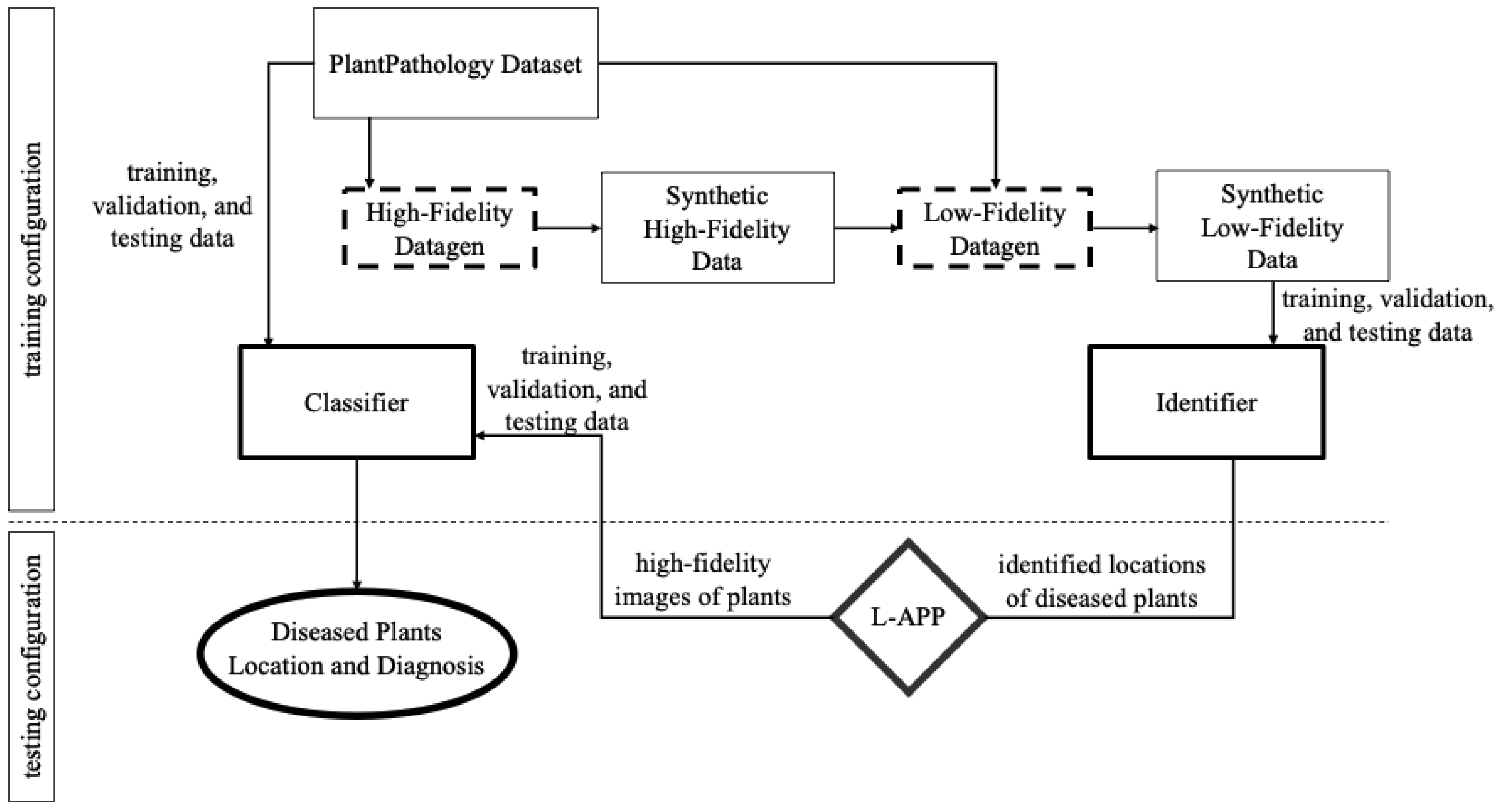
2.1. Data Generation: High-Fidelity Datagen and Low-Fidelity Datagen

2.1.1. High-Fidelity Data Generation

Since the classification task was performed strictly on high-resolution images of diseased plants, training data for this step were simply close-up high-resolution images of diseased plants together with the disease label. The Plant Pathology dataset contains a modest number of such images, but not enough to train the classifier. In addition to the dataset being insufficiently large to train the classifier, it is also plagued by class imbalance, as discussed in Section 3.1. We solved both the data scarcity and class imbalance by augmenting the dataset with a DCGAN.
Because GANs are usually configured to produce images for a single label, multiple GANs were trained so that we could produce novel images of each label. The particular DCGAN instance we used was an industry standard and a brief discussion is given below.
We used an industry-standard GAN to generate additional synthetic high-resolution images of plants and plant diseases. In essence, a GAN works by pitting two networks, a generator and a discriminator, against each other. The generator attempts to create images that will fool the discriminator, while the discriminator attempts to classify images as real or generated. The DCGAN works analogously to a general GAN, with the added clarification that it specifically uses convolution and convolutional-transpose layers in the discriminator and generator, respectively. The analysis was not done on differing levels of effectiveness between various GAN archetypes, but there was no reason to believe another configuration would lead to a much better output or training time than the one used in this paper. We made no changes to the architecture from the original paper by Radford et al. [20].

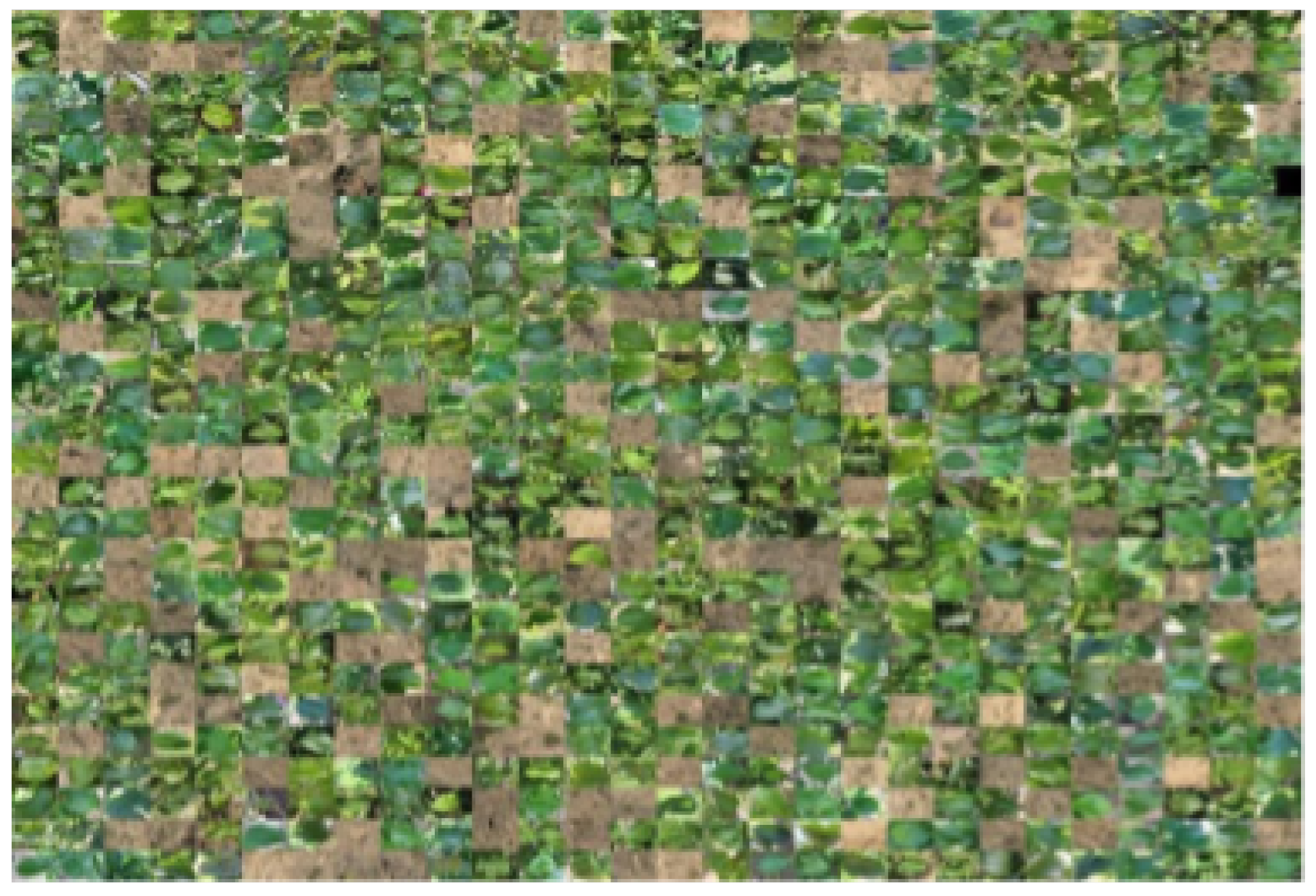
2.1.2. Low-Fidelity Data Generation

The key insight that allowed the full identification and classification model to be trained on a modest number of high-resolution close-up images is that the high/low-resolution division of labor in the identification/classification steps of the model allowed us to take advantage of the high-quality synthetic close-up plant images to generate low-resolution far-field images of whole fields. We developed our new LFD for this purpose and details of our FLD are presented below.
The LFD was a generator which built images representing the pictures a UAV might take while flying over a field by assembling both real and synthetic high-fidelity data images into high-field-of-view images of mock “fields”. These low-fidelity synthetic data were then used to increase the quantity of data available to train, validate and test the model performing the image segmentation task. For each high-field-of-view image, the LFD also output a csv that contained the labels of the locations in the synthetic image of the diseased areas. An example image–csv pair is shown in Figure 2 and Table 1 and described in detail below.
An output image from the LFD was a picture of size 1792 × 1204 pixels. It was divided into 28 rows and columns, with each position holding a 64 × 43-pixel picture of either plant parts or dirt. In our test case, the plant was always a set of apple leaves because our experimental tests were performed on apple orchards. Moreover, the dimensions of the output as well as the subimages were selected to be representative of the hardware in our experimental tests, which was a DJI Mavic 2 Pro 20 feet above the apple canopies, described in Section 2.3.
The subimages that made up an output image were mostly plants, but there were images of soil. These were added to force the identifier to learn how to differentiate foliage with background soil, which are the two main features in an aerial image of an apple orchard. The specific subimage used for the soil was a random slice of a large soil texture. The soils were randomly scattered throughout the images at an approximately 1:5 ratio with images of leaves.
Second, each subimage which contained a plant had a corresponding row in the csv for the overall image. The first column was the id, which was simply the name of the original image. This allowed other applications to find and use those original, full-size images. The second column was the bounding box. This was the location of the subimage represented by that row in the overall image. Finally, the last column was “sick”. These plant images came from the Plant Pathology dataset [10], and were labeled as “healthy”, “rust”, “scab”, or “multiple diseases”. The last three were indicated by a “1” in the corresponding sick column, while a “healthy” image received a 0. Rows were not made for soil images.
After the synthetic data had been processed and augmented into usable low-fidelity training images, we then augmented the low-fidelity dataset by performing operations on images known as cutout and CutMix, which generate new training samples from old by combining two training samples. While we augmented data using both algorithms, CutMix served a more important role as it makes use of the entire image area, and mixes labels so the model can learn to differentiate even within images. We used CutMix on a random basis—for every item in the dataset, there was a 50% chance for the dataset class to load a CutMixed image rather than a normal one.

2.2. Modeling Pipeline: Identifier and Classifier

Once the identifier and classifier were trained, these two models were integrated into a two-step ML application as deployed in the field. We now present this full model’s usage as illustrated in Figure 3. First, using the proper hardware interface, the drone is operated high above the field to capture low-resolution images of the field. In real time, potentially diseased regions of these images are identified, and the drone is maneuvered near the potentially diseased plants to capture high-resolution images of the potentially diseased plants that are passed to the classifier for diagnosis. Since both of the models we used for the image segmentation and image classification tasks of the model were industry standard, we postpone their brief discussion to Section 2.4. The main innovation of this paper is in the way we harnessed the division of labor of the segmentation and classification tasks to facilitate the generation of sufficiently many labeled images for training.

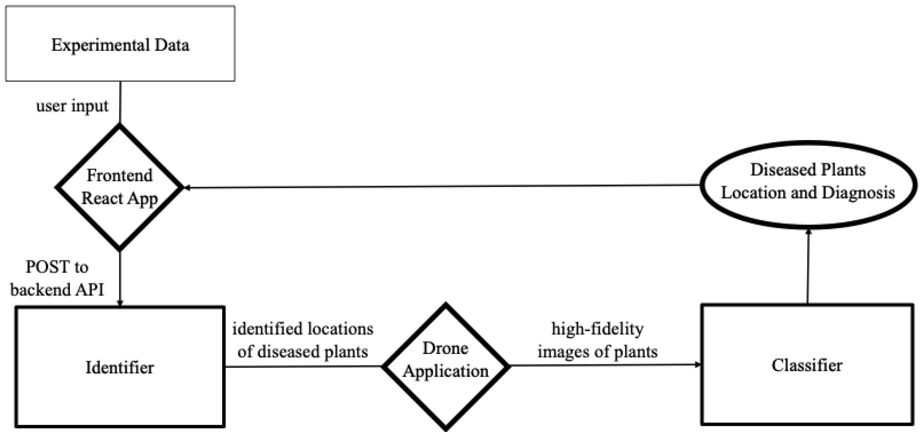
2.3. A Tech Stack Overview

A DJI Marvic 2 Pro drone, one of the most popular drones, was used for validating the proposed system framework. This drone is known to provide a high camera quality and the best obstacle detection among DJI models. Note that our framework can work as is with most DJI models with minor modifications using the DJI API.
A tech stack is the combination of technologies a company uses to build and run an application or project. Sometimes called a “solutions stack”, a tech stack typically consists of programming languages, frameworks, a database, frontend tools, backend tools and applications connected via APIs.
The tech stack used for our system focused on the agility of development that improved flexibility, balance and control in the system. Hence, it helped to maintain and update the system. The three main technologies in our tech stack were: (1) backend tools, (2) frontend tools and (3) applications. The frontend tools included an Android application and a website using the popular state-management framework React.js. As part of managing HTTP requests to the backend API, the system used the Axios library for the React portion of the frontend, and the built-in Volley library for the Android application. Django, a convenient ORM tool, was used for managing the backend SQLite database/endpoint registry. The Django Rest Framework provides an environment in which we can easily create REST APIs. To fully implement Django, a Web server was hosted using Gunicorn through a WSGI entry-point on Heroku. Finally, the library Chakra was used to configure the UI of our React application. The following subsections describe the three main technologies.
The backend tools included three parts: (a) the machine learning applications (i.e., model weight files), (b) the Django REST API using the Django Rest Framework (which allowed our frontend to send HTTP requests to our machine learning applications) and (c) the Django backend itself (which handled the running of the machine learning applications in accordance with the API). Our API consisted of a root containing four subdirectories: one for a list of API endpoint URLs that could be used for an API view that used the model, one for a list of ML algorithms available from the API, one detailing the status of all current ML algorithms, and one that stored the requests for ML algorithms. To serve the intended functionality of our models through the API, the system used endpoints for both the identifier and classifier. These predict views could be accessed by navigating to a REST API, which allowed for POST requests and returned a response for probabilities.
The React Application on the frontend was relatively simple. It served as a tool to make HTTP requests easy in a UI-focused manner. The tool consisted of tabs for standard HTTP request methods including GET, POST, PATCH, PUT and DELETE. This allowed us to test our backend API with ease and additionally allowed us to upload several images to our backend at once, which was especially important to generate results for our experimental data.
The Android DJI Mobile SDK was used for the mobile application development of controlling the DJI Mavic Pro 2 drone. Using the SDK and the Android HTTP request library Volley, the drone can fly over a field while sending HTTP requests for each image frame to the identifier (a backend model that predicts where diseased plants lie in a field) and using the API response to guide the drone. Once the drone is in the correct location to take a photo of the plant, the frame of the image is sent to the classifier, which then returns a diagnosis of the plant to the user.
The system also utilized two software tools for synthetic data generation. The LFD was a generator which built images representing the pictures a UAV might take while flying over a field. These were low-fidelity, high-field-of-view (FOV) images. The HFD was a generator that produced new pictures of plants. These are henceforth referred to as novel images, as opposed to the original images that are found in the Plant Pathology dataset [10].

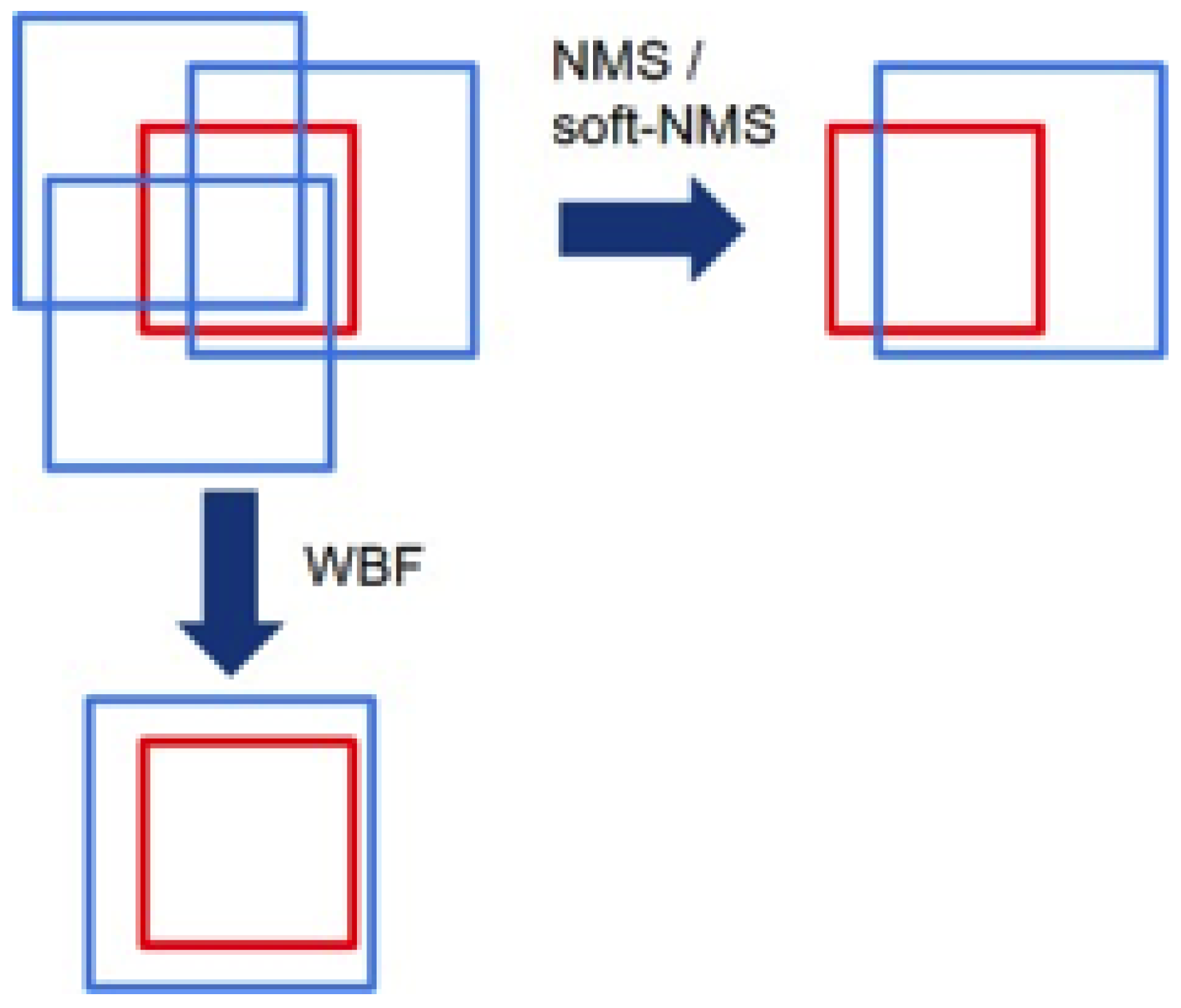
2.4. Computer Vision Tools

For the image classification task, which classified into the disease categories high-resolution images of the potentially diseased regions of the crop fields, we used the EfficientNet architecture, which is an industry standard high-performing image classification network. We used Genetic Efficient Nets for PyTorch [21], which specialize in providing a range of pretrained EfficientNet and MobileNet models in the required PyTorch format. This EfficientNet used a baseline network that was created through a neural architecture search (i.e., an automated architecture engineering scheme) to optimize accuracy and FLOPs. The implementation of this architecture is found at a GitHub repository [21].
For the image segmentation task of isolating potentially diseased regions of the crop field, we used the EfficientDet network, which is an industry high-performing model used for object detection. We selected EfficientDet for the same reason we selected EfficientNet: EfficientDet outcompetes other models due to its remarkable scaling ability and FLOP reduction.
Both EfficientNet and EfficientDet achieve their efficiency using the same compound scaling method that uniformly scales the depth, resolution and width for the backbone and network at the same time. EfficientDet also utilizes EfficientNet backbones due to their efficiency and scalability alongside a weighted bidirectional feature pyramid network (BiFPN) that creates weights while applying feature fusion. This bidirectional pyramid network is intended to solve the problem of other previously used networks which sum features up without distinction, because input features at different resolutions contribute to the output features unequally.

3. Results

3.1. Datasets and Experimental Setup

The real dataset used in this paper was the Plant Pathology 2020 - FGVC7 dataset [10]. It contains 1821 labeled images of plants. The dataset also possesses labels for all these images in csv format. It is important to note that the dataset exhibits a class imbalance. There are 416 (24.17%), 622 (36.14%), 592 (34.40%), and 91 (5.29%) images in the classes healthy, rust, scab, and multiple diseased, respectively. This lack of multiple diseased images as well as healthy images reduces the effectiveness of machine learning models which are trained on these classes. In our experiments, specific high-fidelity images from the real datasets were marked as the test set. These test data were used to evaluate the performance of the model components individually. The results from the individual models were used to estimate the performance of the entire end-to-end model pipeline.
The system was trained on a set of diseases that afflict apple trees. The specific diseases were rust and scab, and there were also healthy and multiple diseased pictures as well. Since the system is essentially a set of machine learning models, it can be used on a wide range of plants/diseases with little to no modification if data for those plants and diseases are easily accessible and of a high quality. We chose apple trees, but our system should be trainable on other plants and diseases if resources for those plants/diseases become available.
We trained our implementation of EfficientDet on the loss function known as summary loss because it required the optimization of both the difference between the bounding-box outputs with their targets (i.e., a box regression loss) and the class outputs with class targets (i.e., a cross-entropy measurement of the classification for each box). An example image–csv pair is shown in Figure 2 and Table 1 in Section 2.1.2. Table 2 shows an example of a slice of training data in csv format.
With a fully trained EfficientDet, trained on synthetic low-fidelity data, we used two additional algorithms to further push the prediction estimates of the identifier. These algorithms were weighted boxes fusion (WBF) alongside test-time augmentation (TTA). The function of the TTA approach is simple—while testing the classifier, augmentations (such as flipping the image or rotating it) are performed, which mimicked the original augmentations performed and then the predictive value is averaged. For the present application this provided a performance boost of approximately five percentage points. Additionally, TTA replaces the need for an ensemble consisting of many models, as it provides several predictions which can be used with the weighted boxes fusion algorithm we used. In our approach, the weighted boxes fusion served as an algorithm to replace the current popular method of merging ensemble boxes, nonmaximum suppression (NMS). In the NMS approach, boxes are considered as belonging to one object if their overlap is higher than a threshold. The issue with this is that it completely disregards the nonoverlap predictions that correspond to the target. However, this changes with a weighted boxes fusion approach: with the WBF, the correct box is picked, but then additional parameters from other semiaccurate boxes are applied to further correct the box, as shown in Figure 4.

3.2. Experimental Results

The performance of the identifier on unseen test data was measured by three statistics: positive confidence level on test data, negative confidence level on test data and accuracy on test data. The performance of the trained identifier is summarized in Table 3.
The classifier was the model that handled the high-fidelity dataset. The goal of the classifier was to return a diagnosis of a plant into one of the following categories: healthy, scab, rust or multiple diseases. The classifier utilized the machine learning framework TensorFlow running on a TPU with data stored in Google Cloud Storage (GCS) buckets. The classifier was much simpler than the identifier.
The data processing started by decoding images to bits and shuffling them into TensorFlow TFRecordDataset objects. Data augmentation was then applied but it was much simpler and only included image flips. To regulate the learning rate, we created a learning rate function which was managed by TensorFlow’s LearningRateScheduler class. We defined the epochs for which learning rate ramped up, was sustained and exponentially decayed, as shown in Figure 5.
To define the model, we used TensorFlow’s implementation of EfficientNetB7, as discussed earlier. We compiled the model using TensorFlow.Keras.Sequential, adding the EfficientNet and an additional final dense softmax layer (with four units). The optimizer we used was the Adam optimizer, which is a stochastic gradient descent method, simply because it is a very robust optimizer that historically performs well in a wide variety of classification problems. Its robustness seems to stem mainly from its use of adaptive learning rates for different parameters, which allowed us to focus more on tuning our architecture and less on particular hyperparameter settings such as learning schedules. Because we were using the softmax activation function, categorical cross entropy was our loss function.
A summary of the performance of the classification component of the model is shown in the confusion matrix for the classifier on unseen test data in Table 4. The performance of the classifier was measured by three statistics, precision, recall and F 1 -Score on unseen test data. The performance of the final trained identifier is sown in Table 5.
Overall, the average accuracy of our classification model was 96.3% and the accuracy of our identifier model was 75.5%. If the performance values were independent of each other, the probability of the full pipeline making a correct diagnosis would be the product of the probabilities of the two individual models, which suggests a full pipeline accuracy of approximately 72.3%. On the other hand, if the samples that the classifier got wrong were disjoint from the samples that the identifier got wrong, the probability of an incorrect diagnosis would be the sum of the probabilities of each step giving an incorrect answer, which suggests a lower bound of 71.8% for the accuracy of the full pipeline. Finally, if the set of the classifier’s errors was contained in the set of errors of the identifier, then the full pipeline accuracy would be equal to that of the identifier, suggesting an upper bound on the full pipeline accuracy of 75.5%.

4. Discussion

At over 70 % , the accuracy of our system seems promising, though ideally one might hope for higher accuracy. This accuracy compares favorably to the typical R 2 values of approximately 0.7 reported in the studies of UAV-enabled potato disease detection [5,6]. We remark that although the classification accuracy metric and the regression coefficient of determination are not directly comparable, all of these values indicate promise but room for improvement. We also remark that the accuracy of our classifier model compares well to the current state of the art reported in Section 1.1 of 95% to 98% on similar tasks. Finally, we remark that the sample size of eight for the multiple disease class used in the evaluation of the classifier in Section 3.2 reduces the statistical significance of the evaluation results for that class. However, since we maintained the class distribution of the real dataset in the evaluation set by using a random sample of 10% of the original data, we were unable to increase the number of multiple diseases images in the evaluation set. In future work, we intend to evaluate the framework on other crops in which instances of multiple diseases are common enough for us to have a more statistically significant sample size for that class.
Furthermore, our framework has two advantages over models common in the literature. First, most of the UAV-based models report classifications or disease-severity ratings on the basis of the entire field, whereas our model reports specific locations of potentially diseased plants. Second, our models are able to train to levels competitive with state-of-the-art models using only a small amount of labeled training data due to our novel data generation algorithms.
For improving our models’ performance in the future, it is clear that the main hindrance to accuracy comes from the identifier. This might be expected because object detection is a much more complicated task than simple n-ary classification, resulting in generally low accuracies even with state-of-the-art models. Therefore, the next step for the improvement of the model accuracy will be to improve the accuracy of the identifier portion of the model. Several approaches could be used here:
  • The first is to address the possibility that the model is relying too heavily on unnatural artifacts present in the low-fidelity synthetic data. Some ways we could accustom the model for this dataset are: (1) more accurately labeling boxes around images so that they do not overlap; (2) the contribution of the pixels at the border of the original image could be increased by adding layers of zeros to the original image (padding) and this would help preserve the information at the borders, recognizing the lack of padding within the low-fidelity data, which we could fix by predicting smaller boxes; and (3) using the classifier to confirm or deny the bounding-box predictions within the identifier.
  • The second big hindrance to the identifier was simply the size of the data. Even optimizing with a GPU, it took around 16 h to run through around 2000 images. This meant we were unable to iterate through a higher-lever optimization of the model including identifying optimal hyperparameters and arrangements of the data augmentation steps. This would have to be addressed through rigorous code optimization because runtime issues are common throughout much of the identifier’s code, especially in places that deal with data.
  • Finally, tests in this paper were conducted on only one crop, apples. For a more complete evaluation of the gains achievable by our framework, it would have to be trained and tested on other major crops. In the present paper, our far-field, low-resolution test data were artificially constructed from real images of diseased and healthy plants. The next step in the direction of obtaining an estimate of the model’s performance in the field with true drone data would be first to collect both far-field low-fidelity drone images of crops and close-up high-fidelity images of both healthy and diseased plants in the low-fidelity drone images. A small set of such images could be augmented to a larger training dataset to train a field model, which would then be tested on a smaller hold-out set of the far-field and associated high-fidelity images. Admittedly, this process would require investment of time and money to generate labeled data, but as demonstrated in this paper, the data requirements of our model are very modest, which would keep training costs minimal.

Author Contributions

Conceptualization, A.P., N.M., M.H. and W.D.B.; data curation, A.P. and N.M.; formal analysis, A.P., N.M., M.H. and W.D.B.; investigation, A.P. and N.M.; methodology, A.P., N.M. and W.D.B.; project administration, A.P. and W.D.B.; resources, A.P. and N.M.; supervision, W.D.B.; validation, Mathew Horak and W.D.B.; visualization, A.P. and N.M.; writing—original draft, A.P., N.M., M.H. and W.D.B.; writing—review and editing, M.H. and W.D.B. All authors have read and agreed to the published version of the manuscript.

Funding

This research received no external funding.

Data Availability Statement

Conflicts of Interest

The authors declare no conflict of interest.

References

  1. FAO. Food and Agriculture Organization of the United Nations: International Plant Protection Convention. Available online: https://www.fao.org/plant-health-2020/about/en (accessed on 17 September 2022).
  2. Barbedo, J.G.A. A review on the use of unmanned aerial vehicles and imaging sensors for monitoring and assessing plant stresses. Drones 2019, 3, 40. [Google Scholar] [CrossRef]
  3. Bock, C.H.; Barbedo, J.G.; Del Ponte, E.M.; Bohnenkamp, D.; Mahlein, A.K. From visual estimates to fully automated sensor-based measurements of plant disease severity: Status and challenges for improving accuracy. Phytopathol. Res. 2020, 2, 9. [Google Scholar] [CrossRef]
  4. Del Ponte, E.M.; Pethybridge, S.J.; Bock, C.H.; Michereff, S.J.; Machado, F.J.; Spolti, P. Standard area diagrams for aiding severity estimation: Scientometrics, pathosystems, and methodological trends in the last 25 years. Phytopathology 2017, 107, 1161–1174. [Google Scholar] [CrossRef] [PubMed]
  5. Duarte-Carvajalino, J.M.; Alzate, D.F.; Ramirez, A.A.; Santa-Sepulveda, J.D.; Fajardo-Rojas, A.E.; Soto-Suárez, M. Evaluating late blight severity in potato crops using unmanned aerial vehicles and machine learning algorithms. Remote Sens. 2018, 10, 1513. [Google Scholar] [CrossRef]
  6. Sugiura, R.; Tsuda, S.; Tamiya, S.; Itoh, A.; Nishiwaki, K.; Murakami, N.; Shibuya, Y.; Hirafuji, M.; Nuske, S. Field phenotyping system for the assessment of potato late blight resistance using RGB imagery from an unmanned aerial vehicle. Biosyst. Eng. 2016, 148, 1–10. [Google Scholar] [CrossRef]
  7. Singh, D.; Jackson, G.; Hunter, D.; Fullerton, R.; Lebot, V.; Taylor, M.; Iosefa, T.; Okpul, T.; Tyson, J. Taro leaf blight—A threat to food security. Agriculture 2012, 2, 182–203. [Google Scholar] [CrossRef]
  8. Gao, D.; Sun, Q.; Hu, B.; Zhang, S. A framework for agricultural pest and disease monitoring based on internet-of-things and unmanned aerial vehicles. Sensors 2020, 20, 1487. [Google Scholar] [CrossRef] [PubMed]
  9. Fasoula, D.A. Nonstop selection for high and stable crop yield by two prognostic equations to reduce yield losses. Agriculture 2012, 2, 211–227. [Google Scholar] [CrossRef]
  10. Thapa, R.; Snavely, N.; Belongie, S.; Khan, A. The plant pathology 2020 challenge dataset to classify foliar disease of apples. arXiv 2020, arXiv:2004.11958. [Google Scholar]
  11. Hughes, D.; Salathé, M. An open access repository of images on plant health to enable the development of mobile disease diagnostics. arXiv 2015, arXiv:1511.08060. [Google Scholar]
  12. Nazki, H.; Yoon, S.; Fuentes, A.; Park, D.S. Unsupervised image translation using adversarial networks for improved plant disease recognition. Comput. Electron. Agric. 2020, 168, 105117. [Google Scholar] [CrossRef]
  13. Joshi, C. Generative Adversarial Networks (GANs) for Synthetic Dataset Generation with Binary Classes. 2020. Available online: https://datasciencecampus.ons.gov.uk/projects/generative-adversarial-networks-gans-for-synthetic-dataset-generation-with-binary-classes/ (accessed on 22 September 2022).
  14. Goodfellow, I.; Pouget-Abadie, J.; Mirza, M.; Xu, B.; Warde-Farley, D.; Ozair, S.; Courville, A.; Bengio, Y. Generative adversarial networks. Commun. ACM 2020, 63, 139–144. [Google Scholar] [CrossRef]
  15. Mirza, M.; Osindero, S. Conditional generative adversarial nets. arXiv 2014, arXiv:1411.1784. [Google Scholar]
  16. Wang, G.; Sun, Y.; Wang, J. Automatic image-based plant disease severity estimation using deep learning. Comput. Intell. Neurosci. 2017, 2017, 2917536. [Google Scholar] [CrossRef] [PubMed] [Green Version]
  17. Kingma, D.P.; Welling, M. Auto-encoding variational bayes. arXiv 2013, arXiv:1312.6114. [Google Scholar]
  18. Perez, L.; Wang, J. The effectiveness of data augmentation in image classification using deep learning. arXiv 2017, arXiv:1712.04621. [Google Scholar]
  19. Simonyan, K.; Zisserman, A. Very deep convolutional networks for large-scale image recognition. arXiv 2014, arXiv:1409.1556. [Google Scholar]
  20. Radford, A.; Metz, L.; Chintala, S. Unsupervised representation learning with deep convolutional generative adversarial networks. arXiv 2015, arXiv:1511.06434. [Google Scholar]
  21. Wightman, R. Genetic Efficient Nets for PyTorchs. 2021. Available online: https://github.com/rwightman/efficientdet-pytorch (accessed on 22 September 2022).
Figure 1. An overview of data generation and modeling framework.
Remotesensing 14 04765 g001
Figure 2. An example image output from the LFD.
Remotesensing 14 04765 g002
Figure 3. The pipeline with identifier and classifier.
Remotesensing 14 04765 g003
Figure 4. A demonstration of outcomes from NMS and WBF approaches given TTA predictions (as a replacement for ensemble predictions). Red represents ground truth, and blue represents TTA predictions.
Remotesensing 14 04765 g004
Figure 5. Epoch (x-axis) versus learning rate (y-axis).
Remotesensing 14 04765 g005
Table 1. An example csv format output from the LFD.
idbboxClass Label
Train_1609.jpg[64, 0, 64, 43]1
Train_1028.jpg[128, 0, 64, 43]1
Train_354.jpg[192, 0, 64, 43]1
Train_1082.jpg[256, 0, 64, 43]0
Train_10.jpg[320, 0, 64, 43]1
Train_1280.jpg[384, 0, 64, 43]1
Train_463.jpg[448, 0, 64, 43]1
Train_1178.jpg[512, 0, 64, 43]1
Table 2. A slice of training data in csv format.
Image_id# Healthy# Multiple_Diseases# Rust# Scab
Train_0.jpg0001
Train_1.jpg0100
Train_2.jpg1000
Train_3.jpg0010
Train_4.jpg1000
Train_5.jpg1000
Train_6.jpg0100
Train_7.jpg0001
Train_8.jpg0001
Train_9.jpg1000
Train_10.jpg0010
Table 3. Identifier’s summarized results.
TestAverage PositiveAverage NegativeAccuracy
Summary LossConfidence on Test DataConfidence on Test DataOn Test Data
1.891420.549980.204680.75466
Table 4. Confusion matrix on test data for the classifier.
Healthy (p)Rust (p)Scab (p)Multiple Diseases (p)Sum
Healthy (a)4700047
Rust (a)1550056
Scab (a)0052153
Multiple diseases (a)12148
Note: A (p) label indicates the predicted class while an (a) label indicates the actual class.
Table 5. Classifier performance metrics.
PrecisionRecall F 1 -ScoreSupport
Healthy0.961.000.9847
Rust0.960.980.9756
Scab0.980.980.9853
Multiple diseases0.800.500.628
Note: Support shows the number of samples predicted to be in that class within the test set and can be used as an indicator for the accuracy of other metrics.
Publisher’s Note: MDPI stays neutral with regard to jurisdictional claims in published maps and institutional affiliations.

