Deep Learning-Based Automatic Extraction of Cyanobacterial Blooms from Sentinel-2 MSI Satellite Data

Abstract

Cyanobacterial harmful algal blooms (CyanoHABs) in inland water have emerged as a major global environmental challenge. Although satellite remote sensing technology has been widely used to monitor CyanoHABs, there are also some automatic extraction methods of CyanoHABs based on spectral indices (such as gradient mode, fixed threshold, and the Otsu method, etc.), the accuracy is generally not very high. This study developed a high-precision automatic extraction model for CyanoHABs using a deep learning (DL) network based on Sentinel-2 multi-spectral instrument (MSI) data of Chaohu Lake, China. First, we generated the CyanoHABs “ground truth” dataset based on visual interpretation. Thereafter, we trained the CyanoHABs extraction model based on a DL image segmentation network (U-Net) and extracted CyanoHABs. Then, we compared three previous automatic CyanoHABs extraction methods based on spectral index threshold segmentation and evaluated the accuracy of the results. Based on “ground truth”, at the pixel level, the F1 score and relative error (RE) of the DL model extraction results are 0.90 and 3%, respectively, which are better than that of the gradient mode (0.81,40%), the fixed threshold (0.81, 31%), and the Otsu method (0.53, 62%); at CyanoHABs area level, the R² of the scatter fitting between DL model result and the “ground truth” is 0.99, which is also higher than the other three methods (0.90, 0.92, 0.84, respectively). Finally, we produced the annual CyanoHABs frequency map based on DL model results. The frequency map showed that the CyanoHABs on the northwest bank are significantly higher than in the center and east of Chaohu Lake, and the most serious CyanoHABs occurred in 2018 and 2019. Furthermore, CyanoHAB extraction based on this model did not cause cloud misjudgment and exhibited good promotion ability in Taihu Lake, China. Hence, our findings indicate the high potential of the CyanoHABs extraction model based on DL in further high-precision and automatic extraction of CyanoHABs from large-scale water bodies.

1. Introduction

Rapid economic and societal development, along with the increasing impact of climate change, have rendered inland water eutrophication a major environmental challenge globally [1,2]. Harmful algae blooms (HABs) are extreme manifestations of water eutrophication, such as cyanobacterial harmful algal blooms (CyanoHABs) and are the most prominent inland water blooms [3]. Cyanobacteria have a bubble-like structure that allows them to adjust their distribution at different water depths by changing their buoyancy [4]. CyanoHABs are formed by rapid growth and reproduction of cyanobacteria, which float and accumulate on the water surface, resulting in environmental pollution while endangering human welfare [5,6].

Satellite remote sensing technology has been widely used to monitor CyanoHABs in inland water because of its advantageous monitoring speed and range, compared to traditional field sampling and monitoring methods [7,8]. CyanoHABs have similar reflectance spectral characteristics to vegetation. For example, reflection peaks occur in the green band, while relatively low reflectance occurs in the red band; the reflectance in the near-infrared band rises to form a reflection platform that differs significantly from the reflectance spectrum of water. This near-infrared reflectance is the main basis for the satellite remote sensing identification of CyanoHABs. Therefore, CyanoHAB region extraction can be achieved via threshold segmentation of a single band reflectance or spectral index constructed by the correlated band [9]. The common bands and spectral indexes for recognizing CyanoHABs are as follows: the near infrared band [10,11,12], normalized difference vegetation index (NDVI) [13,14], enhanced vegetation index (EVI) [15,16], floating algae index (FAI) [17], and adjusted FAI (AFAI) [18,19].

Determining an appropriate threshold is crucial to accurately extracting CyanoHABs using spectral indexes; however, the extraction threshold for different images depends on shooting time, observation angle, weather conditions, water turbidity, water surface roughness, and other factors. With fewer images, the optimal segmentation threshold of each image can be determined through visual interpretation based on the false color composite image [20]; however, this is not a suitable strategy for the rapid processing of numerous images and may be affected by the subjective judgment of different operators. To extract CyanoHABs from a large number of images, researchers have used the fixed-threshold method [21,22,23,24], but this method can produce large errors when applied to multiple images. Recent studies have tried to automatically obtain extraction thresholds for different images using different methods including the gradient mode method [22], bimodal threshold method [18,25], and Otsu method [26]. However, these methods have limitations and cannot address all the challenges of the image threshold, resulting in low extraction accuracy of CyanoHABs [27]. To better determine the segmentation threshold of CyanoHABs with higher precision and automation, Hou et al. [27] calculated the commission international de L’Eclairage (CIE) color space coordinates based on the visible light band of the remote sensing images and extracted the green areas, which were considered CyanoHABs. While this method facilitates the determination of the threshold, it is easily distracted by green water bodies; thus, the extraction accuracy of CyanoHABs is reduced because it does not use the most obvious near-infrared band high reflection spectral feature that distinguishes CyanoHABs from ordinary bodies of water. Therefore, although remote sensing has been used to monitor CyanoHABs for over three decades, a more efficient high-precision and automatic extraction method has yet to be developed.

As a novel approach, deep learning (DL) has been widely used in contemporary remote sensing research because it can extract multi-scale and multi-level features from remote sensing images, and aid in ground feature classification and target recognition [28,29,30,31], including land cover classification [32,33], water distribution extraction [34], cloud recognition [35], and coral reef identification [36]. DL can comprehensively utilize the spectral and textural features of HABs in satellite remote sensing images and has been successfully applied to HAB recognition, such as in the monitoring of Sargassum [37], Karenia brevis [38], and Ulva prolifera [39] in coastal waters. Meanwhile, the DL image segmentation network has shown excellent image segmentation performance on remote sensing images, which can also extract HABs from high-resolution images. For example, Wang et al. used the image segmentation network to train and predict Sentinel-2 MSI images and automatically extracted images of Sargassum in the Gulf of Mexico [40]. The investigated HABs based on DL and MSI were mainly macroalgal blooms. Sentinel-2 multi-spectral instrument (MSI) has 13 bands, which can extract the spectral characteristics of HABs; and its high spatial resolution allows the clear depiction of the texture characteristics of HABs. It may have potential application in extracting CyanoHABs based on a DL image segmentation network and MSI. However, compared with macroalgal blooms, microalgal blooms show a gradual change from a low to a high aggregation state in water. Thus, it is more difficult to extract CyanoHABs. Current research on the DL and MSI-based extraction of microalgal blooms, such as CyanoHABs in inland waters, is scant. High-precision CyanoHAB annotation datasets and DL-based CyanoHAB extraction models are not easily found. Thus, the applications of DL and MSI in this respect needs to be studied further.

Facing the problem of high-precision and automatic extraction of CyanoHABs in inland water, this study attempted to build a CyanoHABs extraction method based on DL image segmentation network. We took the Chaohu Lake in China (where CyanoHABs occur frequently) as the study area, and Sentinel-2 MSI as remote sensing data source. Firstly, CyanoHABs dataset was generated by visual interpretation; then, we used dataset to train the CyanoHABs recognition model based on DL semantic segmentation network (U-Net) and test the extraction results; finally, we compared with other common automatic CyanoHABs extraction methods.

2. Study Area and Data Description

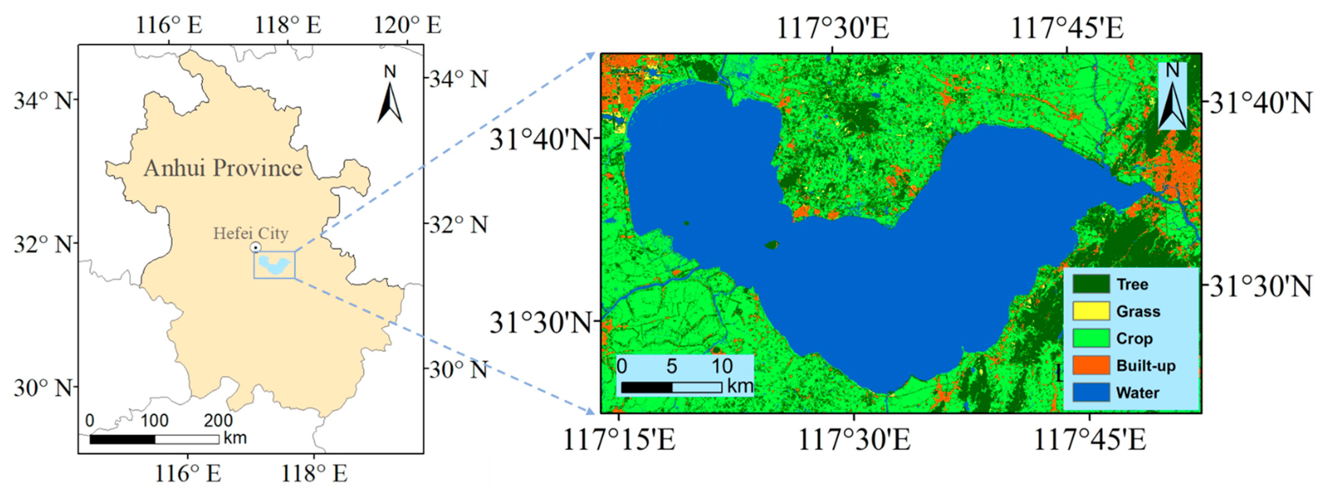
2.1. Study Area

The Chaohu Lake (31°25′–31°43′N, 117°17′–117°51′E; Figure 1; the landcover around Chaohu Lake was downloaded from European Space Agency) is located in the center of Anhui Province and is the fifth largest freshwater lake in China. The Chaohu Lake has an average water level of 8 m, with an area of 770 km², and an average water depth of 3 m [41,42]. There are 35 rivers distributed around the Chaohu Lake in a centripetal shape, including the Nanfei, Shangpai, and Hangbu rivers. In the past 40 years Chaohu Lake has developed one of the most serious issues of eutrophication with the highest frequency of CyanoHABs in China, possibly due to the rapid development of the surrounding economy and society [43,44].

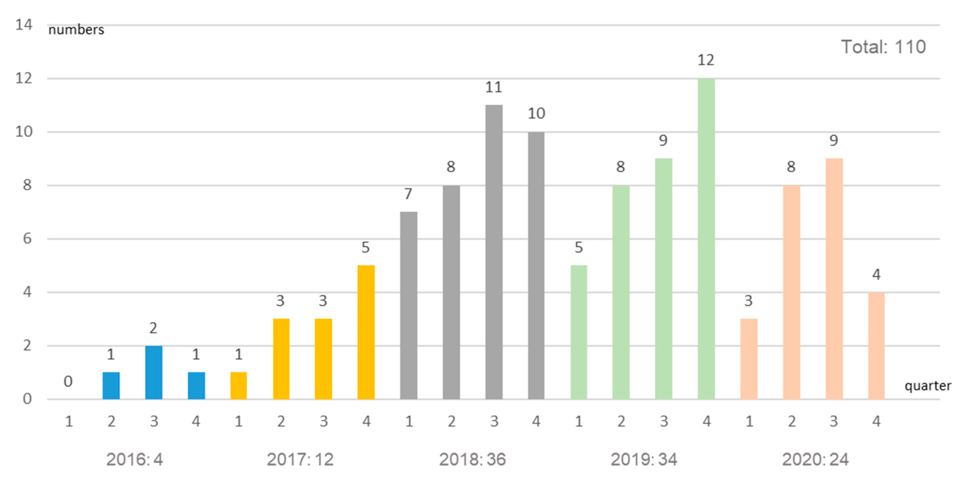
2.2. Data Description

In this study, Sentinel-2 MSI image data of the Chaohu region from 2016 to 2020 were obtained from the official website of the European Space Agency (ESA; https://scihub.copernicus.eu/dhus/#/home, accessed on 22 September 2022). Sentinel-2 data included those from Sentinel-2A, launched on 23 June 2015, and Sentinel-2B, launched on 7 March 2017. The temporal resolution of dual satellite networking was five days, and it included three spatial resolution bands of 10, 20, and 60 m. The bands with a 10 m resolution included Band 2 (Blue, 490 nm), Band 3 (Green, 560 nm), Band 4 (Red, 665 nm), and Band 8 (NIR-1, 842 nm); the bands with a 20 m resolution included Band 5 (Red Edge, 705 nm), Band 6 (Red Edge, 740 nm), Band 7 (Red Edge, 783 nm), Band 8A (NIR-2, 865 nm), Band 11 (SWIR-1, 1610 nm), and Band 12 (SWIR-2, 2190 nm); and the bands with a 60 m resolution included Band 1 (443 nm), Band 9 (945 nm), and Band 10 (1375 nm). Notably, the three 60-m resolution bands had low spatial resolution and did not contain the characteristic bands of CyanoHABs. Therefore, only the bands with 10 and 20 m spatial resolution were used in this study. Additionally, ESA provided two downloadable data types: atmospheric apparent reflectance product with ortho correction and geometric fine correction (L1C) and bottom-of-atmosphere corrected reflectance product (L2A), which was only available from 2018 onwards. We manually selected the thumbnails of the images of the Chaohu Lake area released by ESA one by one based on visual observation, and downloaded all the images with little or no cloud coverage over Chaohu Lake, termed ‘effective images’. Finally, 110 MSI images of Chaohu Lake were obtained and sorted on a quarterly and yearly basis in Figure 2.

3. Methods

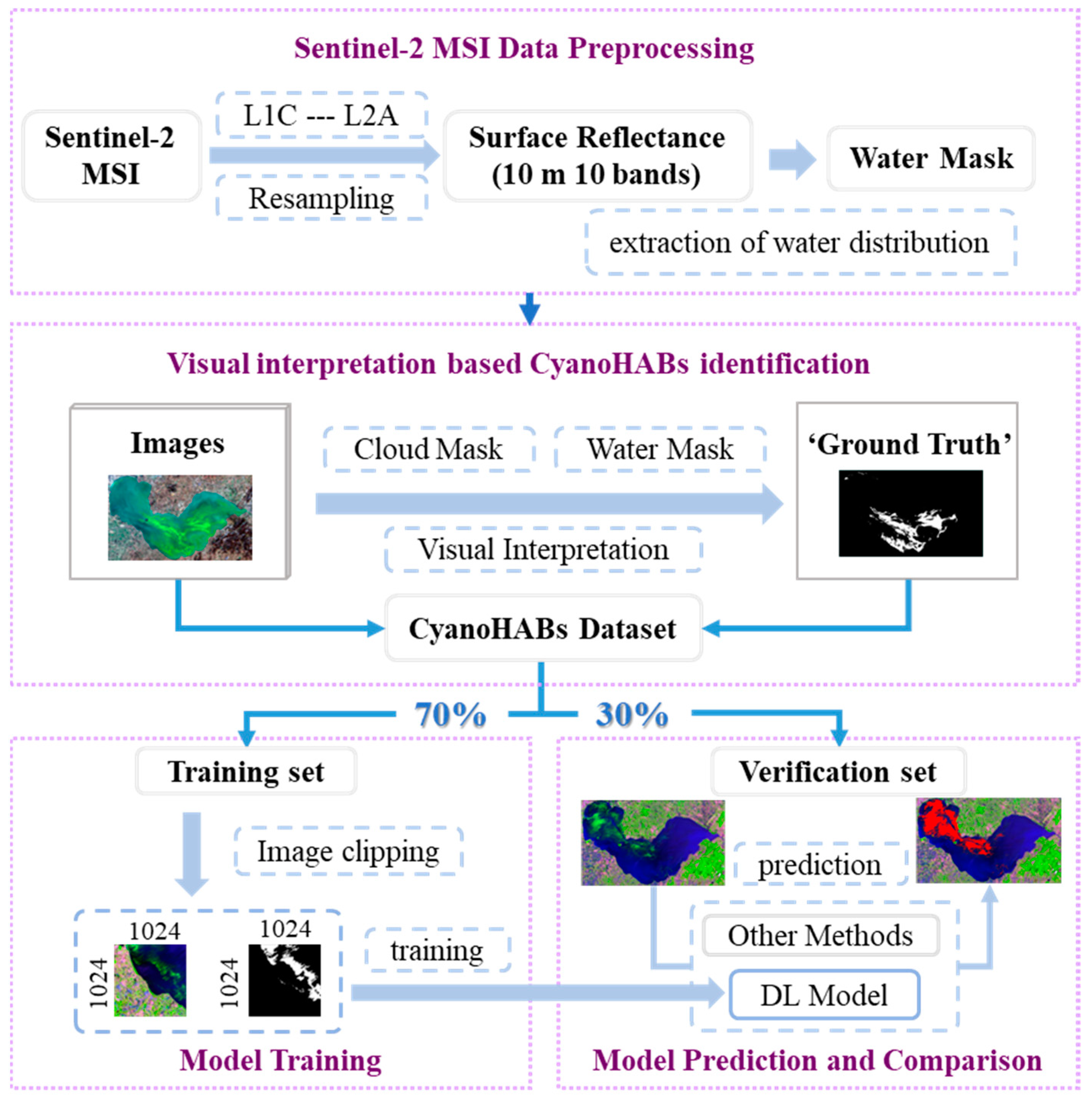
3.1. Overall Technical Process

Figure 3 details the workflow followed during this study. First, the original Sentinel-2 MSI data were pre-processed to obtain 10 bands of surface reflectance with 10 m resolution and a water mask. Subsequently, cloud recognition was carried out, after which the CyanoHABs of each image were accurately extracted by combining spectral indexes and visual interpretation to generate the CyanoHABs dataset. Then, we divided the dataset into a training set and verification set by a 7:3 ratio, and the training set was clipped into 1024∗1024 size subsets for model training based on a DL network. Finally, based on the validation set, the accuracy of the DL network-based model predicting the results was evaluated and compared with other previous automatic CyanoHABs extraction methods.

3.2. Sentinel-2 MSI Data Pre-Processing

The data requirements for subsequent experiments in this study were a 10-band surface spectral reflectance data at a spatial resolution of 10 m. The pre-processing of the original Sentinel-2 MSI data included three steps: atmospheric correction of L1C data, band resampling and image mosaicking of L2A data, and extraction of water distribution.

Since the first scene L2A data over the Chaohu Lake provided by the European Space Agency were from December 18, 2018, and the dataset before this were the L1C products, atmospheric correction of L1C to L2A data was necessary. This correction process was completed using the official Sen2Cor plugin setting command line (L2A_Process). The calculation model of Sen2Cor was built by LibRadtran laboratory using the theoretical model of atmospheric radiation transmission and MSI sensor and other parameters. We then used SNAP (Ver. 7.0; Cre. ESA; Loc. France.) to resample the 20-m bands into a 10-m spatial resolution by nearest neighbor interpolation. Two Sentinel-2 images were required for the complete coverage of the Chaohu Lake area; therefore, image fusion and cutting of the Chaohu Lake area was also conducted. Finally, since land features were complex, especially vegetation, and compared to water, they could easily be misjudged as CyanoHABs, we extracted the water distribution. In this study, a modified normalized difference water index (MNDWI) [45] threshold segmentation was used to extract water distribution, as follows:

$$MNDWI=\frac{r\left(Green\right)-r\left(SWIR\right)}{r\left(Green\right)+r\left(SWIR\right)}$$

(1)

where ρ (Green) and ρ (SWIR) refer to the reflectivity of green band (Band 3: 560 nm) and shortwave infrared band (Band 11: 1610 nm), respectively.

Owing to the high frequency of CyanoHABs in the Chaohu Lake, they could be easily misjudged as land in the MNDWI images; thus, the distribution range of water body calculated with a single image was not accurate. However, the water body distribution range of the Chaohu Lake changed only slightly in a year, thus, the obtained annual water boundary of could be applied to the CyanoHAB extraction for all images in that year. Therefore, the first step was to calculate the MNDWI index of each image and automatically obtain the water distribution based on the Otsu method [46]. In the second step, the water distribution of each image in a year was superimposed, the probability that each pixel was divided into water was calculated, and the pixels with a probability greater than 20% were retained as the annual water distribution of the Chaohu Lake to avoid false extraction interference of water in a small number of images. In the third step, the obtained water distribution edge was eroded inward by three pixels to reduce the influence of geometric correction error and land adjacency on water extraction. According to Figure 2, the number of effective images between 2016 and 2017 was much less than that of the subsequent three years; therefore, the 2016–2017 images jointly produced the water body distribution.

3.3. Extraction of “Ground Truth” of CyanoHABs Based on Visual Interpretation

Obtaining accurate extraction results of CyanoHABs (i.e., “ground truth”) was the premise of the DL model training and evaluation. As the CyanoHABs change rapidly in the water, it is impossible to obtain a lot of “ground truth” data through in situ investigation. However, CyanoHABs can show clear spectral and texture features different from the water on the images, so the “ground truth” was generally determined based on the visual interpretation [26,27,40]. Therefore, this study extracted the “ground truth” of CyanoHABs based on visual interpretation.

3.3.1. Cloud Recognition

Compared with the background water body, cloud pixels showed strong signals on FAI images, which could be easily misjudged as CyanoHABs; therefore, cloud recognition preprocessing operations were required before CyanoHABs extraction. As clouds have stronger reflectance in the shortwave infrared band, they can be removed by threshold segmentation of the shortwave infrared band. In this experiment, we found that the shortwave infrared reflectance of some highly concentrated CyanoHABs was higher than those of a small number of thin cloud and cloud edge pixels. If the segmentation threshold was set too low, the highly concentrated CyanoHABs would be wrongly eliminated as clouds. After statistical analyses and comparison, we finally elected to use ρ (Swir-2: 2190 nm) > 0.085 which eliminated the interference of most cloud pixels. For a small number of thin clouds and cloud edge pixels that may be misjudged as CyanoHABs, the scene-by-scene manual modification method was adopted.

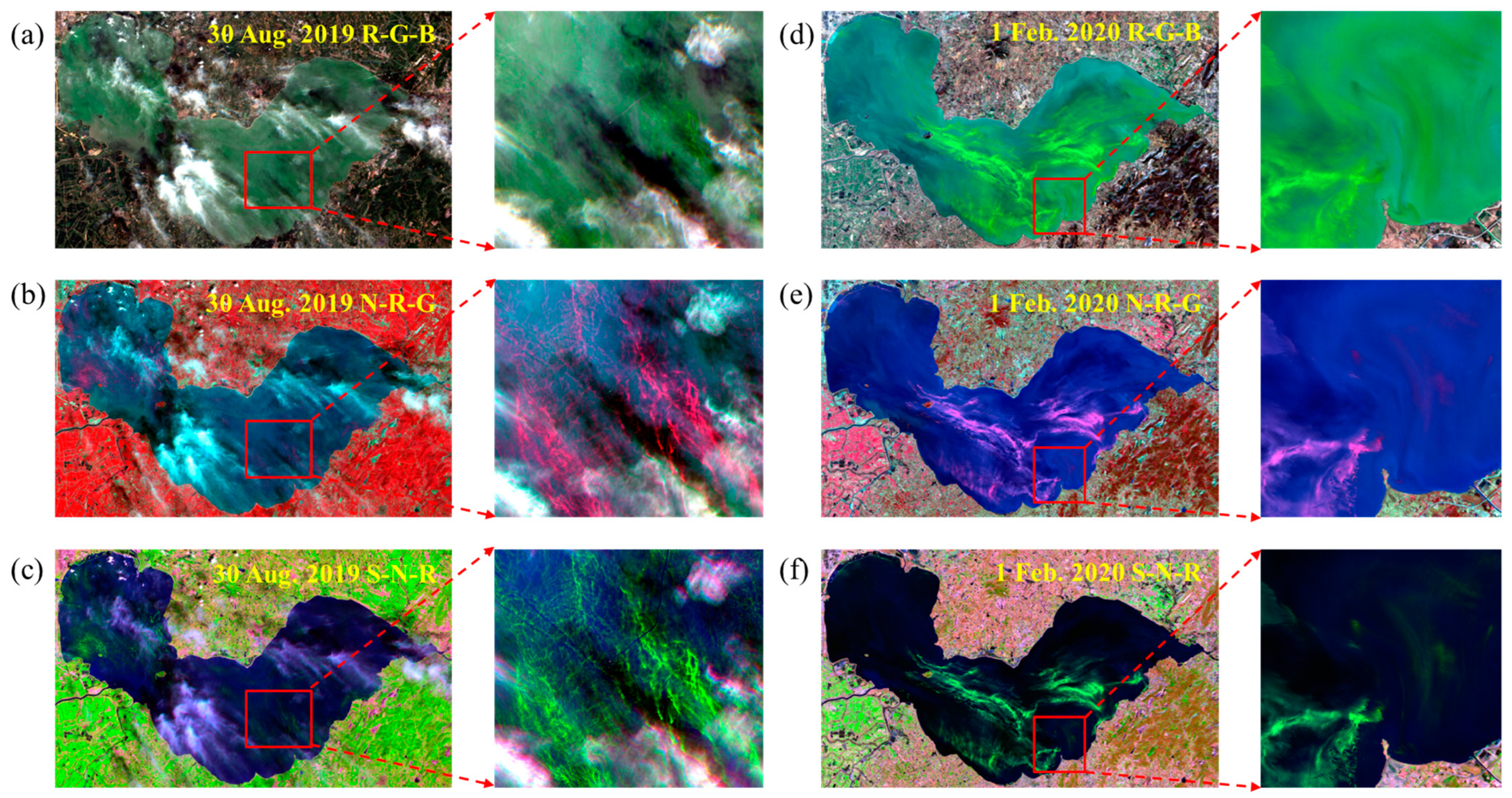
3.3.2. Extraction of CyanoHABs Based on FAI Threshold Determined by Visual Interpretation

FAI was first proposed by Hu (2009) to extract floating algal blooms, which has become a common spectral index for extracting CyanoHABs. It is defined as the vertical distance between the near infrared band and the connecting line between the red and shortwave infrared bands [17]. Different from ordinary algal blooms usually suspended in the water, cyanobacteria have a bubble-like structure and usually float and accumulate on the water surface [4]. Therefore, the spectral characteristics of CyanoHABs were mainly determined by the cyanobacterial cells and have high reflectance in the near-infrared band [9]. However, the spectral characteristics of ordinary algal blooms were mainly determined by both algal cells and pure water. Due to the high absorption of pure water, the reflectance of ordinary algal blooms in the near-infrared band are not as high as those of CyanoHABs. Therefore, the FAI, which is based on the high near infrared reflectance, can effectively distinguish CyanoHABs from ordinary algal blooms. Furthermore, many studies have shown that the algal blooms in Chaohu Lake were CyanoHABs, and no other ordinary algal blooms [5,14,43,47]. FAI was originally defined as follows:

$$FAI=R_{rc,NIR}-R_{rc,NIR}^{\prime }$$

(2)

$$R_{rc,NIR}^{\prime }=R_{rc,RED}+(R_{rc,SWIR}-R_{rc,RED})·\frac{{\lambda }_{NIR}-{\lambda }_{RED}}{{\lambda }_{SWIR}-{\lambda }_{RED}}$$

(3)

where $R_{rc,RED}$, $R_{rc,NIR}$, and $R_{rc,SWIR}$ represent Rayleigh corrected reflectance in red, near infrared, and shortwave infrared bands, respectively. Furthermore, ${\lambda }_{RED}$, ${\lambda }_{NIR}$, and ${\lambda }_{SWIR}$ represent the red, near infrared, and shortwave infrared band central wavelengths, respectively. In this study, surface reflectance data is used instead of Rayleigh corrected reflectance. Band 4 (665 nm), Band 8 (842 nm), and Band 11 (1610 nm) of Sentinel-2 MSI data are selected as the red, near infrared, and shortwave infrared, respectively.

To ensure the extraction accuracy of CyanoHABs, the extraction threshold was determined via visual interpretation. For remote sensing images, different image stretching and color composite methods could affect the human judgment on the extraction threshold of CyanoHABs. Therefore, before determining the threshold, we needed to determine a unified image display method to ensure that all images were under the same visual interpretation standard. Comparing the standard true color synthesis (R: red; G: green; B: blue), the standard false color composite (R: near infrared; G: red; B: green), and the false color composite of three bands used in FAI (R: shortwave infrared; G: near infrared; B: red), we found that in the latter image, the CyanoHABs appeared bright green and the water body appeared dark blue or black. The CyanoHABs show significant different color from the ordinary water body, also have distinctive texture features (Figure 4). Therefore, we used bands B11 (1610 nm), B8 (842 nm), and B4 (665 nm) for the false color composite method of all images, and we uniformly chose the 2% linear stretching method.

The specific process of visual extraction began by calculating the FAI of the image and conducting cloud and land masking. Thereafter, we set the FAI segmentation threshold in the interval to [–0.02, 0.1] with the step of 0.001 to extract the CyanoHAB areas with each threshold. The extraction results obtained by each threshold were then superimposed on the false color composite map to form a series of CyanoHAB extraction images. We visually inspected the extracted area scene by scene according to the sequence of FAI threshold from low to high and selected the threshold of the most appropriate extraction results as the best extraction threshold. To reduce the subjective effect of visual interpretation, we arranged two experts with extensive experience in extracting CyanoHABs by visual interpretation to determine the final “ground truth” data together. Finally, the FAI image was segmented according to the optimal threshold to generate the CyanoHABs extraction binary image, in which the “CyanoHABs” pixels were assigned as one and the “non CyanoHABs” pixels were assigned as zero. The extracted result via visual interpretation was then regarded as the “ground truth” for training and validating automatic CyanoHABs extraction methods. The “ground truth” which corresponded to the individual original surface reflectance image to form the Chaohu CyanoHABs dataset. We randomly divided the dataset into a training set (77 scenes) and a verification set (33 scenes). The training set will be used to train the CyanoHABs extraction DL model, and the verification set will be used for accuracy evaluation and method comparison.

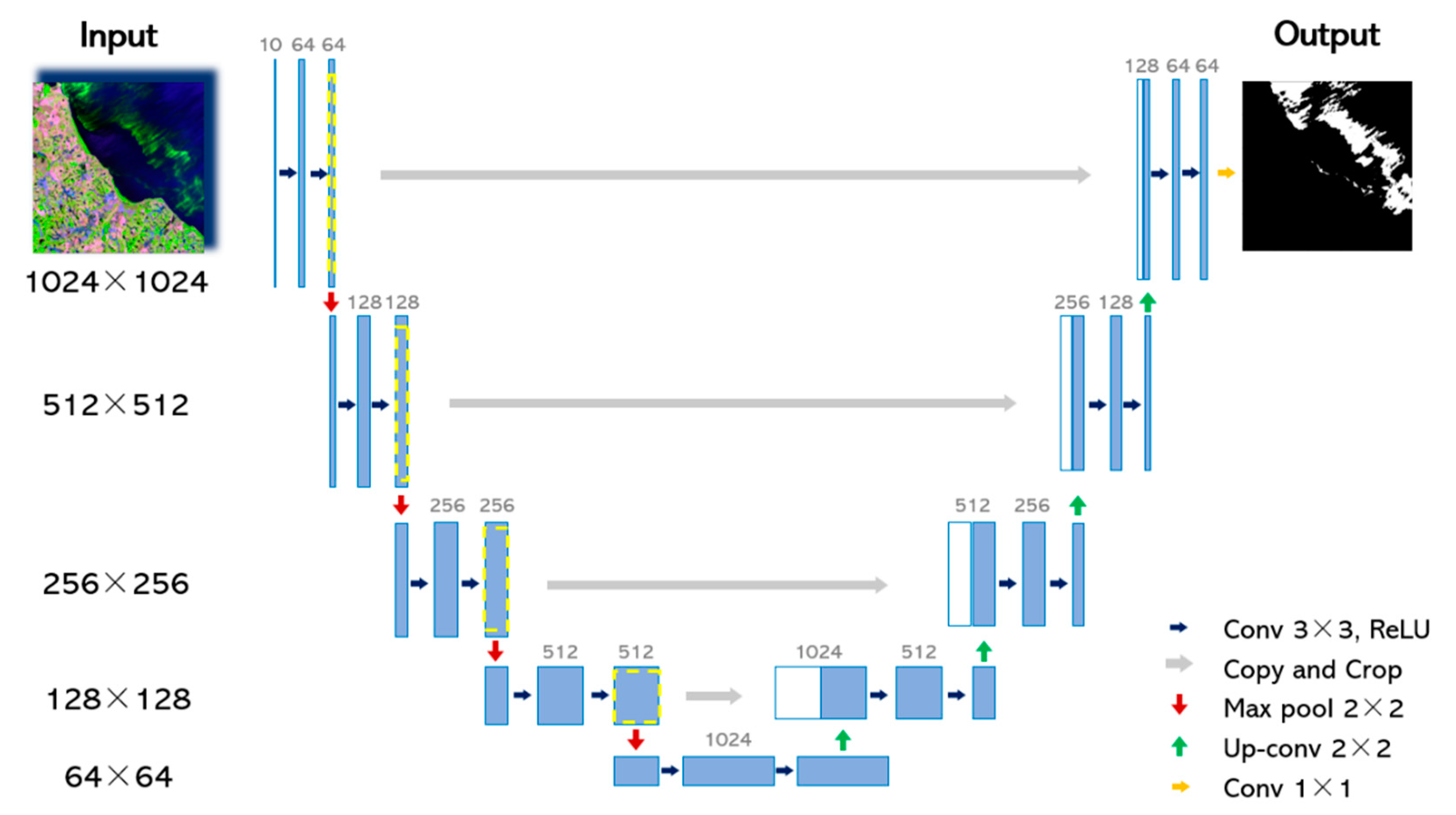
3.4. Training of CyanoHABs Extraction Model Based on DL

DL is a new research direction in the field of machine learning (ML), which utilizes complex algorithms and structures to learn the deep internal laws and representation features of sample data. Currently, it has achieved remarkable image recognition and classification results. DL mainly involves a convolutional neural network (CNN), sparse auto encoder neural network (SANN), and deep belief network (DBN). CNN refers to the feed forward neural network with convolution operation and depth structure and is the most widely used algorithm in remote sensing image semantic segmentation processing [48]. Image semantic segmentation refers to the classification at the pixel level, which requires that the input and output are grid data and the size of the characteristic image at the input end is variable. The algorithm generated by CNN through full convolution construction design can solve this problem [49].

Extracting CyanoHABs means classifying the CyanoHAB pixels into one category, which can be regarded as image semantic segmentation. There are various types of image semantic segmentation networks, among which, U-Net is the classic network [50] widely used in remote sensing [51,52]. This network designs a U-shaped architecture, which can obtain context and location information simultaneously. The pixel level classification of images can be determined through the encoder–decoder structure. In this study, we used U-Net to train the CyanoHABs extraction model. Figure 5 shows that the structure of the network consisted of a contracting path (left side) and an expansive path (right side). The contracting path consisted of the repeated application of two 3 × 3 convolutions, each followed by a rectified linear unit (ReLU) and a 2 × 2 max pooling operation. The number of feature channels doubled for each down sampling. Each step in the expansive path included up-sampling of feature mapping. The number of feature channels for each up sampling was halved and the image size was doubled until it was finally restored to the original image size. The model input was a 10-band surface reflectance image with an image size of 1024 × 1024 (obtained by clipping the original image, henceforth the sub image, and the clipped label was thereafter called the sub label), and the output of the model was a single band binary diagram, where “CyanoHABs” were represented by “1” and “non CyanoHABs” were represented by “0”.

We used the binary classification cross entropy loss function (BCEloss) as the loss function of this network, which involved two objectives (i.e., “CyanoHABs” and “non CyanoHABs”) and was equivalent to a binary classification task, expressed as follows:

$$Loss=-(y·\log (p)+(1-y)·\log (1-p\left)\right)$$

(4)

where, in the case of the two classifications, there were only two cases for the final prediction result of the model, either a positive or negative example; p represents the probability that the prediction result is a positive example; 1 − p represents the probability that the prediction result is a negative example; and y is the sample label. If the sample belonged to a positive example, the value would be 1, otherwise, 0.

We used an adaptive moment estimation (Adam) optimizer [53] for model optimization. During the DL model training, the model parameters were updated and changed at various times, and the learning rate represented the magnitude of each parameter update. The learning rate was not invariable and needed to decay gradually with the number of trainings to achieve the best convergence effect of the model. In this study, our initial learning rate was set to 0.0002, and the learning rate was gradually reduced by Cosine annealing [54]. The training and prediction of this study were carried out on the same computer equipped with Intel(R) Xeon(R) Gold 6128 CPU @ 3.4 GHz and NVIDA GeForce RTX 3090 GPU.

3.5. Prediction of CyanoHABs Based on the DL Model

The original images were cut into sub-images of 1024 × 1024 for consistent input image size in the prediction of CyanoHABs during the model training. However, the prediction accuracy decreased with the image edge, because of the “boundary effect” [55], which resulted in the jagged boundary of the prediction result. Therefore, the sub-images were prepared using a redundant edge strategy, i.e., 16 pixels were cut outward in four directions and only the prediction results of 1024 × 1024 in the image center were spliced.

Ultimately, the length and width of the original Lake Chaohu images were not exact multiples of 1024. To ensure that each position of the original image could also be cut into 1024 × 1024 sub-images, we expanded the length and width of each band of the original images to a multiple of 1024 in four directions, and then expanded it further by 16 pixels. The expanded pixel values were supplemented according to the “edge filling” method, i.e., the pixel values of the nearest neighboring region were selected. In the sub-image predictions, the “sliding window prediction” was executed from the upper left corner to the right and then to the lower side of the expanded images with 1056 × 1056 as the clipping area and 1024 as the step size. After the sub-images were predicted, the prediction results were spliced together, the central ranges of the length and width of the original images were also cut out from the stitched result images as the prediction results of the original Chaohu images.

To avoid misjudgment of some land features, we also conducted water mask processing on the basis of the prediction results, i.e., the land area of the water bloom prediction result image was assigned 0, resulting in a better prediction effect of CyanoHABs. The model prediction process is shown in Figure 6.

3.6. Accuracy Evaluation

3.6.1. Accuracy Evaluation Indexes for Model Training

During DL-based CyanoHABs extraction model training, it is necessary to divide the training set into training and verification subsets and optimize the model through iterative training. The indexes for evaluating the model accuracy include the Mean Intersection over Union (MIoU) and the Kappa coefficient.

MIoU is the standard model evaluation index in semantic segmentation task [56]. It calculates the ratio of the intersection and union of the “ground truth” set and predicted segmentation set, where best performance is indicated by a value of 1. For the binary classification task of this study, the calculation formula of MIOU can be simplified as follows:

$$MIOU=\frac{1}{2}\sum _{i=1}^2\frac{P\cap T}{P\cup T}$$

(5)

where P represents the prediction result area of each category and T represents the real value result area of each category.

Kappa coefficient is an index used for consistency testing. In the classification problem, it can detect if the predicted results of the model are consistent with the actual classification results [38]. The closer it is to 1, the higher the accuracy of the model. For the binary classification task, it can be expressed as follows:

$$Kappa=\frac{p_o-p_e}{1-p_e},$$

(6)

$$p_e=\frac{a_1\times b_1+a_2\times b_2}{2\times 2}$$

(7)

where p_o is the overall classification accuracy, that is, the total number of pixels correctly classified in each category divided by the total number of pixels in all categories; a₁ and a₂ represent the number of “ground truth” pixels in each category and b₁ and b₂ represent the number of pixels predicted in each category.

3.6.2. Accuracy Evaluation Indexes for Model Prediction

We used the optimized model to predict the CyanoHABs in verification set images and evaluated the accuracy of CyanoHABs extraction results from three aspects based on “ground truth”.

First, accuracy evaluation indexes based on pixel level, including precision (P), recall (R), F1 score (F1), and relative error (RE).

$$P=\frac{TP}{TP+FP}$$

(8)

$$R=\frac{TP}{TP+FN}$$

(9)

$$F1=2·P·\frac{R}{P=R}$$

(10)

$$RE=\frac{|T-P|}{T}\times 100\%$$

(11)

where TP (True Positive) refers to the number of correctly predicted CyanoHABs pixels, FP (False Positive) refers to the number of falsely predicted CyanoHABs pixels, FN (False Negative) refers to the number of falsely predicted non-CyanoHABs pixels, T refers to the number of CyanoHABs pixels in the ground truth dataset, and P refers to the number of CyanoHABs pixels in the prediction result. Among them, the best performance of P, R, and F1 is 1, and RE is 0%.

It should be noted that we can calculate a set of accuracy evaluation indexes based on each image; however, there will would be large errors in the evaluation index for the images with few or no CyanoHABs pixels, although these have little effect on extraction results. Therefore, to overcome this problem, we added the number of pixels of all verification images to calculate total accuracy evaluation indexes.

Second, we calculated the accuracy evaluation indexes based on the extracted CyanoHABs area level. We used “x” to represent the CyanoHABs areas of the “ground truth” and “y” to represent the CyanoHABs areas of the prediction results and performed linear fitting on the scattered points generated by each image. The linear fitting slope showed the difference between the prediction result and the true value; the closer it was to 1, the better the prediction effect. R² showed the robustness of the prediction model; the closer it was to 1, the better the robustness.

Third, we calculated the accuracy evaluation indexes based on the extracted CyanoHABs frequency map level. We extracted the CyanoHABs of each Chaohu Lake image from 2016 to 2020, and then superimposed and calculated the outbreak frequency map of CyanoHABs. The frequency map was defined as the number of images recognized as CyanoHABs per pixel/the number of images recognized as water and bloom per pixel (excluding clouds and land). Comparing the frequency map of the prediction results with the “ground truth” frequency map, the prediction accuracy of the model could be evaluated on the spatiotemporal scale.

3.6.3. Other Comparison Methods

We compared three other previous automatic extraction methods of CyanoHABs, including gradient mode [22], fixed threshold, and Otsu method based on FAI, and then evaluated the accuracy of the prediction results of each method based on verification set.

In the gradient mode method [22], the 3 × 3 gradient operator was used to traverse the FAI image and generate the FAI gradient map. The gradient at a point indicated that the operator had the maximum change rate along the direction at that point; thereafter, the land and cloud pixels were removed through a mask, and pure water and pure water bloom pixels were removed through the empirical threshold of FAI image. Thereafter, the histogram of the remaining FAI gradient pixels (i.e., the mixed pixels of CyanoHABs and water) was extracted and the mode of remaining gradient gray histogram pixels (gradient mode) was calculated. Finally, the average FAI value of the image pixels corresponding to the gradient mode was calculated, which was then taken as the segmentation threshold of CyanoHABs in this image.

With the fixed threshold method, a unified FAI threshold was used for all the images to extract the CyanoHABs.

In the Otsu method [46], according to the gray distribution characteristics of the image, it was divided into two parts: background and target. As variance is one of the measures of gray distribution uniformity, the variance within the category should ideally be the lowest for the same category and the variance between background and target should be the highest. The segmentation threshold can be determined when the inter class variance is the highest. In this study, the threshold of FAI image was obtained based on the Otsu method.

These methods automatically obtain the extraction threshold of CyanoHABs in each image. After obtaining the threshold, threshold segmentation should be performed on the whole image, and the water mask should be superimposed to obtain the final CyanoHABs extraction result.

4. Results

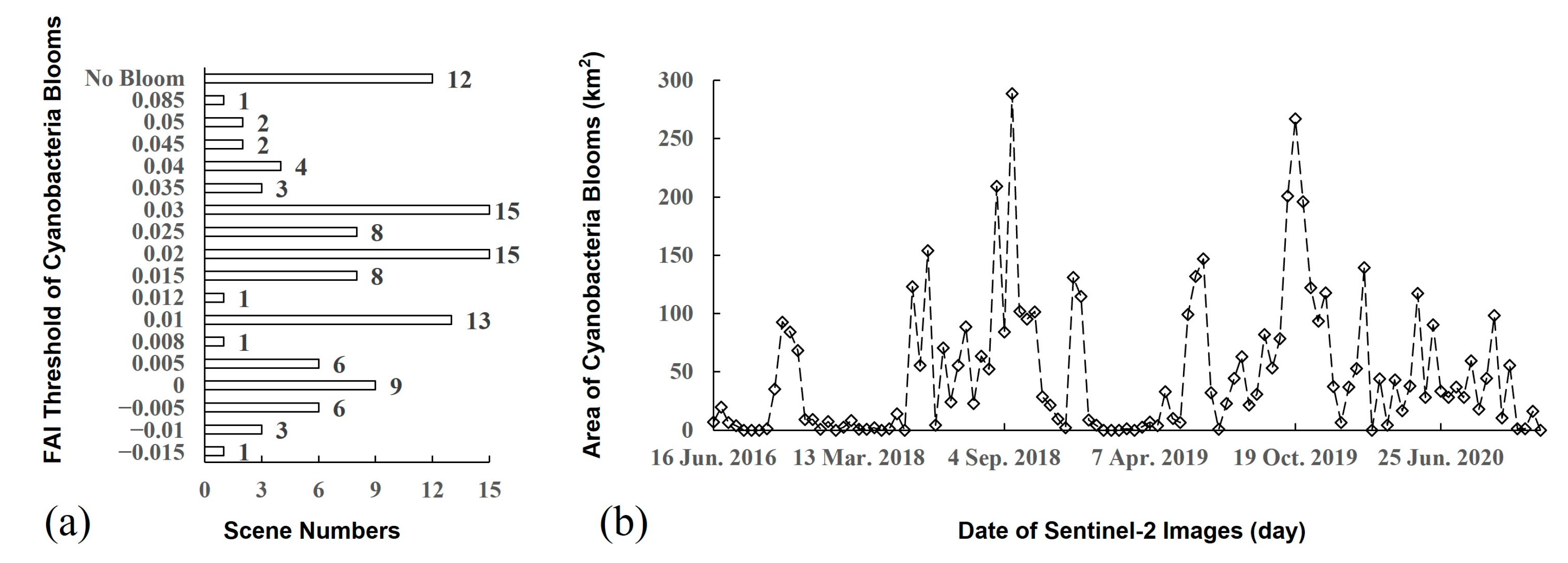
4.1. CyanoHABs Extraction Results Based on Visual Interpretation

The CyanoHABs extraction threshold distribution of the 110 FAI images was between −0.015 and 0.085 based on the extraction results of visual interpretation (Figure 7a). In addition, each pixel represented 0.1 km² according to the spatial resolution of the Sentinel-2 MSI images. Between 2016 and 2020, the minimum outbreak area of CyanoHABs was 0.6155 km² (on 26 July 2019) and the maximum outbreak area was 288.4538 km² (on 19 September 2018), of which 12 images did not contain any blooms (Figure 7b). The original image of the training set and the “ground truth” (i.e., label) were cropped into 1024 × 1024 sub-images and sub-labels. These sub-images and sub-labels were then used for DL model training. A total of 500 pairs were selected, of which 12 typical image pairs are shown in Figure 8. The verification set was used to predict the model and evaluate the accuracy of the prediction results.

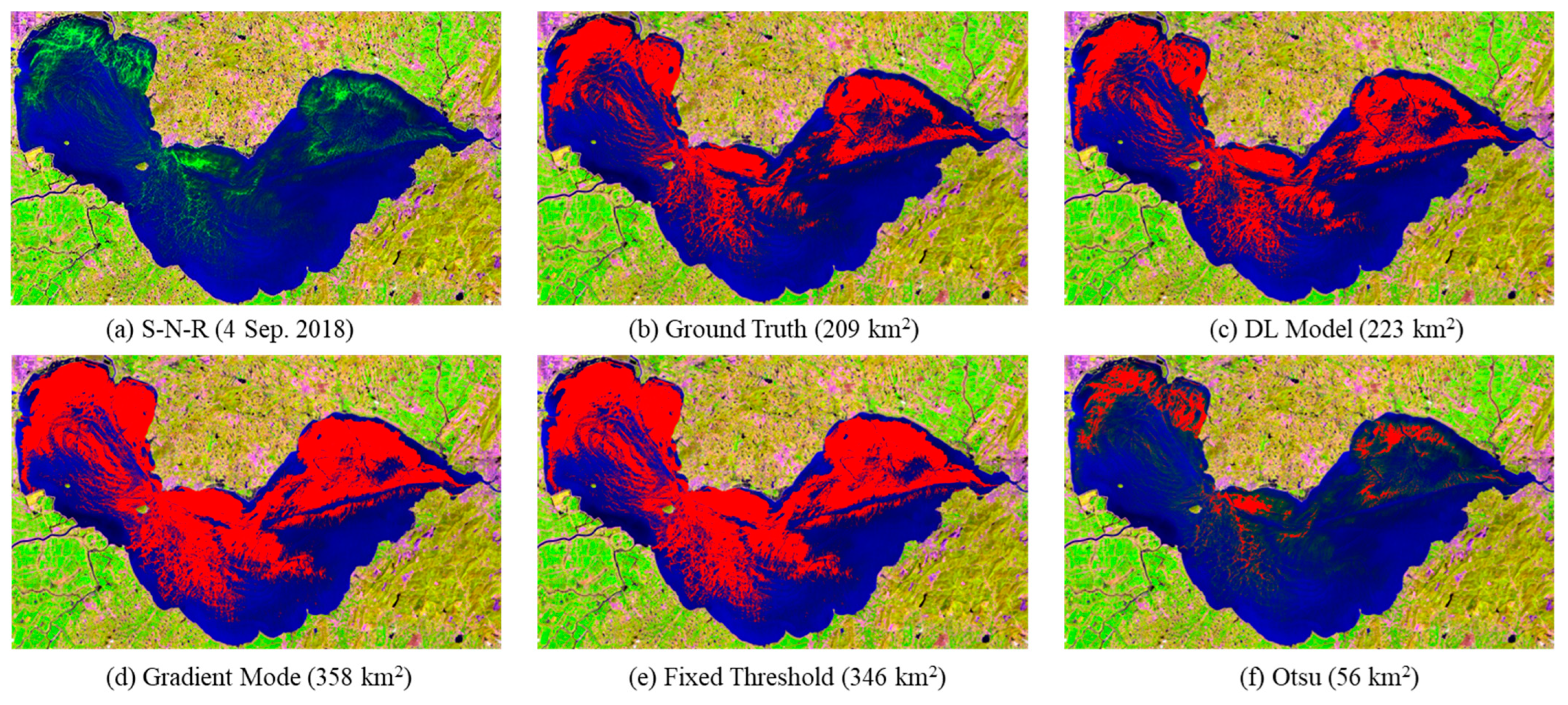
4.2. CyanoHABs Extraction Results Based on Automation Methods

4.2.1. CyanoHABs Extraction DL Model and Results

We trained 500 pairs of sub-images and sub-labels according to the methods detailed in Section 3.4 and conducted 5000 iterations. Model training and validation were randomly divided according to a 7:3 ratio. Thereafter, the model performance had stabilized, and the loss function had decreased to ~0.025. The MIOU of the final model was 0.8583, the class IOU was 0.9846 for the background and 0.7320 for the CyanoHABs, and Kappa was 0.8375. Generally, the model was found to have high accuracy and was suitable for the prediction of CyanoHABs.

Similarly, we performed the model prediction of surface reflectance images according to the method in Section 3.5 and obtained the prediction results of CyanoHABs of each image. Figure 9c show the extraction results of CyanoHABs based on DL model in the Chaohu Lake.

4.2.2. CyanoHABs Extraction Parameters Based on Other Comparison Methods

For the gradient mode method, according to the results of FAI threshold determined visually, the FAI threshold values of the Chaohu pure water and pure water bloom pixels based on Sentinel-2 MSI surface reflectance image were 0.005 and 0.05, respectively. Subsequently, different segmentation thresholds of CyanoHABs were calculated for each image.

For the fixed threshold method, the best threshold of the training set image determined by visual interpretation was determined and the average value of 0.017 was considered as the CyanoHABs extraction threshold of the verification set image.

Figure 9 d–f shows the extraction results of CyanoHABs based on the gradient mode method, the fixed threshold method, and the Otsu method, respectively, in the Chaohu Lake. The CyanoHABs extracted by gradient mode and fixed threshold method were 358 km² and 346 km², respectively, which shows that both of them have high false mention of CyanoHABs, while the Otsu method misses more (just 56 km²), and DL model (223 km²) is the closest to the visual “ground truth” (209 km²).

4.3. Accuracy Evaluation and Comparison

We used the DL model trained in this study, as well as the gradient mode, the fixed threshold, and Otsu method to predict the CyanoHABs in the verification set, and then evaluated the accuracy of the prediction results.

4.3.1. Accuracy Evaluation on the Pixel Level

From the pixel-based accuracy evaluation index (

Table 1. Accuracy evaluation indexes of different methods.

Methods	Recall	Precision	F1-Score	RE
DL Model	0.89	0.91	0.90	3%
Gradient Mode	0.97	0.69	0.81	40%
Fixed Threshold	0.94	0.72	0.81	31%
Otsu	0.36	0.95	0.53	62%

), the F1-score of the prediction result of the DL model was the highest at 0.90, and the RE was the lowest at only 3%, indicating the highest accuracy of the DL model among the several comparison methods. The F1-score obtained by the gradient mode method and the fixed threshold method were both 0.81, while the low precision (0.69, 0.72) indicated high false judgment rate for CyanoHABs. The F1-score obtained by the Otsu method was low (0.53), and low recall indicated a high misjudgment rate of this method.

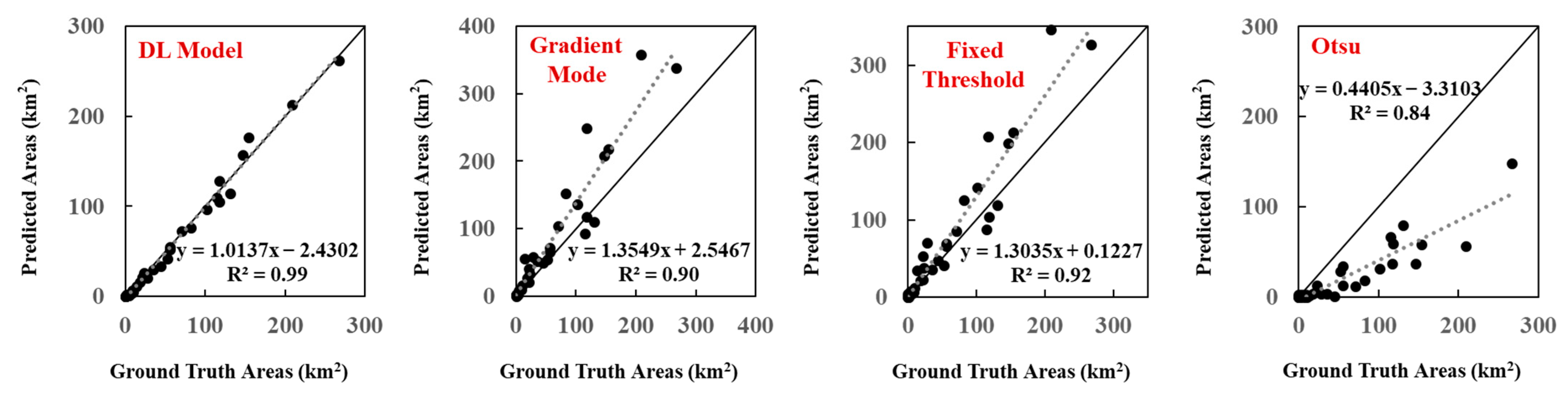
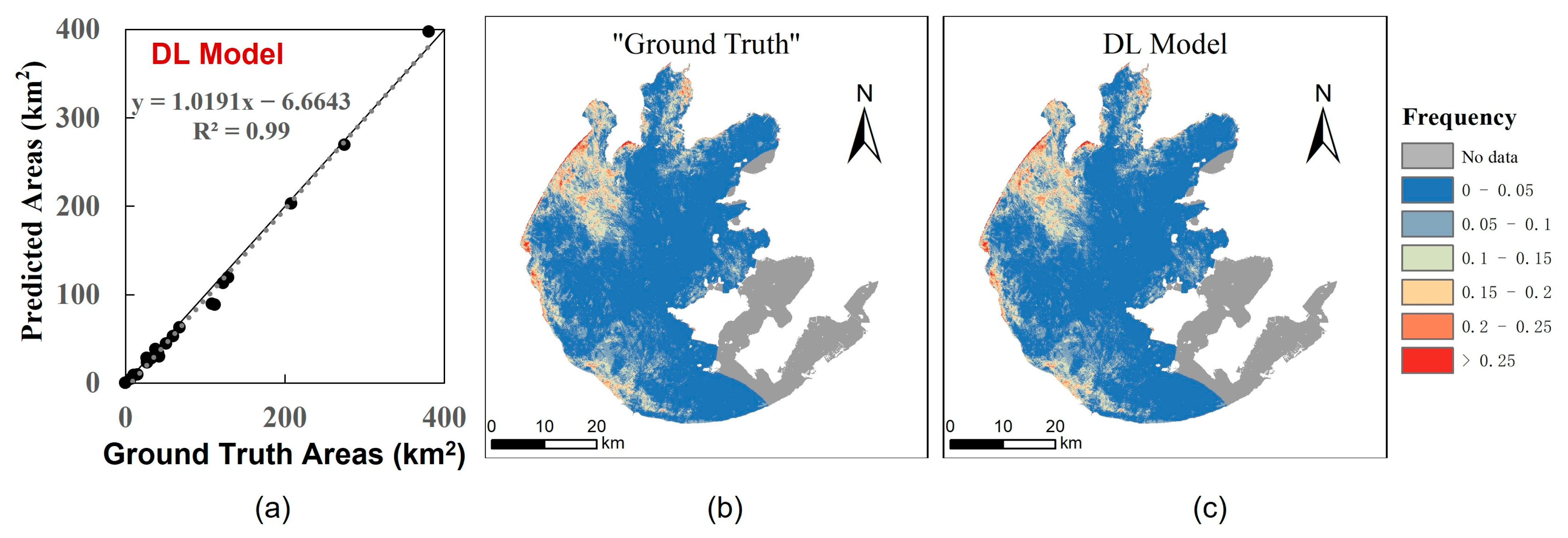
4.3.2. Accuracy Evaluation on Area Level

We evaluated the CyanoHABs extraction area of the prediction results of the validation set obtained by different methods (Figure 10). For the results by the DL model, each point was distributed around the 1:1 line, with a linear fitting slope of 1.0137, and R² of 0.99, indicating that the prediction results of the model fit well with the “ground truth”. Among the three comparison methods, most of the points obtained by the gradient mode method and the fixed threshold method were distributed above the 1:1 line, and with the linear fitting slopes of 1.3549 and 1.3035, respectively, indicating that the area predicted by the two methods were higher than that judged by visual interpretation. The Otsu method points were distributed below the 1:1 line, with a linear fitting slope of 0.44, indicating a low overall predicted area.

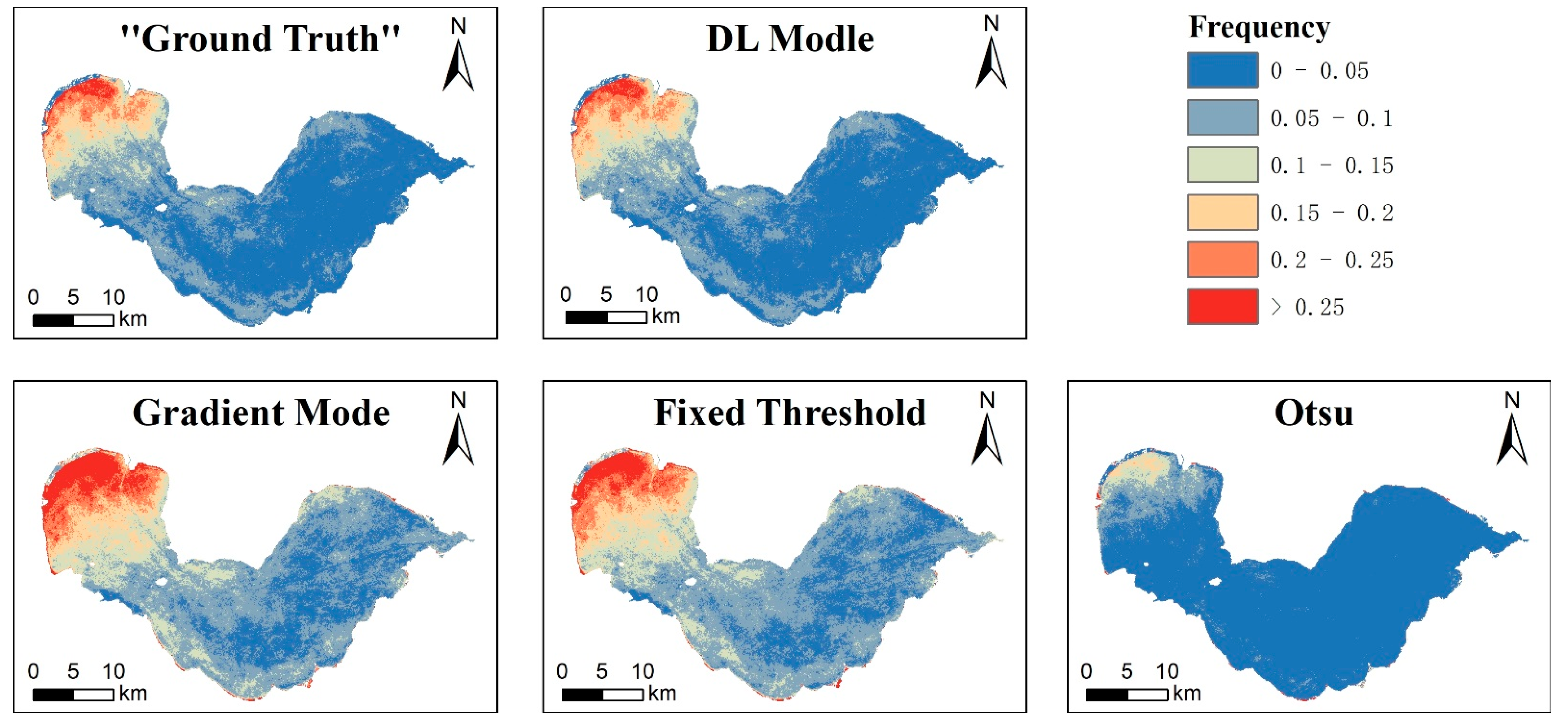
4.3.3. Accuracy Evaluation on Long Time Series Frequency Map Level

The frequency map of CyanoHABs in the Chaohu Lake between 2016 and 2020 were generated based on the “ground truth” values of the 110 images. Similarly, the prediction results of different methods were also used to produce the frequency map of CyanoHABs (Figure 11). According to the value and frequency distribution, the frequency map predicted by the DL model was more consistent with the spatiotemporal distribution characteristics of CyanoHABs in the “ground truth” frequency map. The frequency map of the gradient mode and the fixed threshold methods showed higher outbreak frequency of CyanoHABs than that of the “ground truth”, while that of the Otsu method was lower.

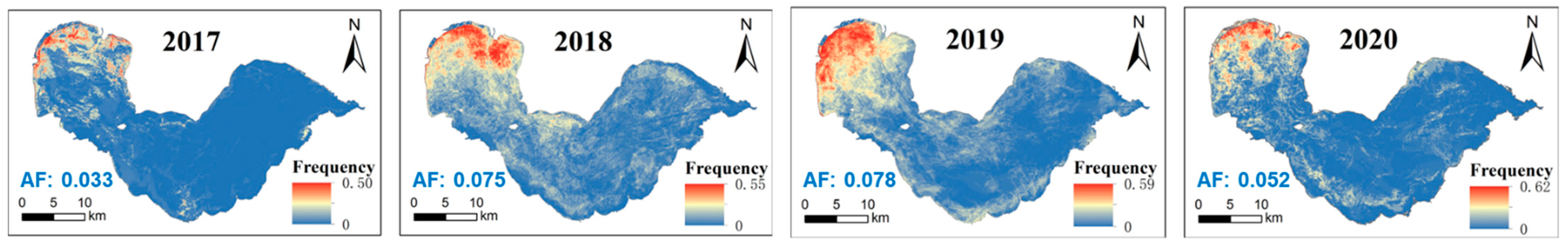
4.4. Spatial and Temporal Change Analysis of CyanoHABs

We calculated the average outbreak frequency of CyanoHABs throughout the entirety of Chaohu Lake every year, and generated the annual CyanoHABs outbreak frequency map (Figure 12). Spatially, the frequency of CyanoHABs was basically the same every year, which primarily occurred in the western section of Chaohu Lake, particularly on the northwest bank, was significantly higher than that in the central and eastern sections of the lake. In terms of time, the average frequency (AF) of CyanoHABs in Chaohu Lake was lowest in 2017 at 0.033, with increased frequency in 2018 and 2019, with an AF of 0.075 and 0.078, and it did not decrease until 2020 to an AF of 0.052.

5. Discussion

5.1. Applicability of the DL Model

The model generated in this study was solely based on the samples of CyanoHABs in the Chaohu Lake. To verify the applicability of the model, we also applied this model to Taihu Lake, which has also been afflicted by a serious outbreak of CyanoHABs. The data used included 21 scenes of Sentinel-2 L2A images of cloudless and less cloudy scenes in Taihu Lake in 2019. The “ground truth” value of the CyanoHABs in Taihu Lake was determined by visual interpretation and predicted using the DL model. The accuracy of the model prediction results was also evaluated based on the “ground truth”.

Unlike Chaohu Lake, the aquatic vegetation was widely distributed in the east coast of Taihu Lake. The vegetation has similar spectral characteristics to those of the CyanoHABs and could be easily misjudged as CyanoHABs. As there were few CyanoHABs on the east side of Taihu Lake [8,57], we generated a mask to eliminate the interference of aquatic vegetation in this area. The CyanoHABs “ground truth” was then extracted by visual interpretation after cloud and land shielding.

We directly applied the DL model from Chaohu Lake to predict the CyanoHABs in Taihu Lake. The results, after shielding the aquatic vegetation and land, were evaluated based on the “ground truth” images. The evaluation indexes also included recall, precision, F1, and RE for pixel level, scatter fitting map for area level, and frequency map for frequency level. The pixel-based evaluation results of Taihu Lake showed that the R² was 0.82, P was 0.86, F1 was 0.84, and RE was 5%. Although the accuracy was not as good as that in Chaohu Lake, the results were satisfactory. In the area scatter fitting map (Figure 13a), each point was distributed around the 1:1 line, with a linear fitting slope of 1.02, and an R² of 0.99, indicating consistency with the area obtained by visual interpretation. The frequency map of the “ground truth” and the mode prediction results were consistent (Figure 13b,c). The comprehensive evaluation indexes of the three aspects of the Taihu Lake proved that the DL model based on the Chaohu Lake dataset could be applied in images without aquatic vegetation.

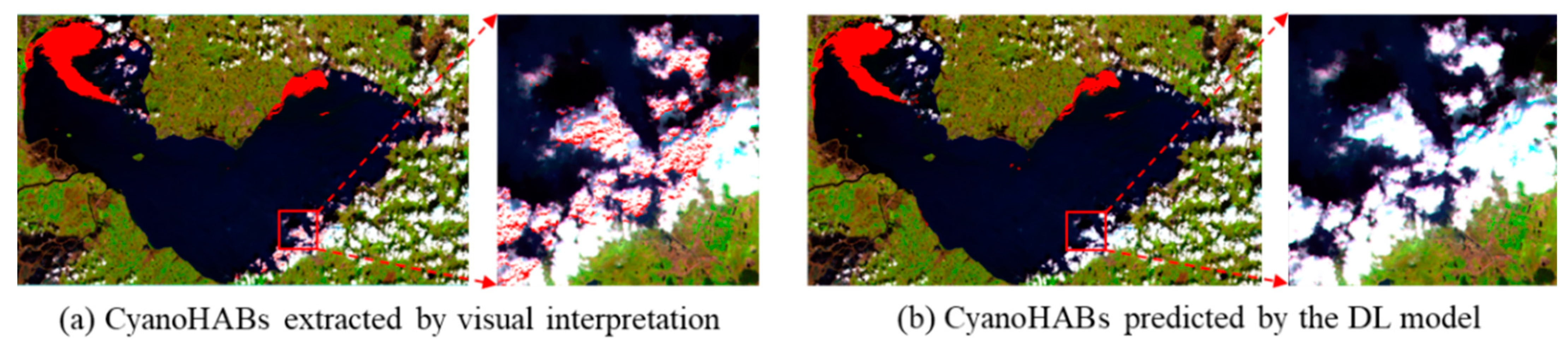
5.2. Sensitivity of the DL Model to Clouds

Cloud recognition is traditionally a necessary step in the CyanoHABs extraction method due to the strong reflection signal of cloud pixels on FAI images. Taking the image of Chaohu Lake on September 28, 2020, as an example, we first determined the optimal threshold of FAI based on visual interpretation, and then extracted CyanoHABs based on threshold segmentation. As shown in Figure 14a, some clouds were misjudged as CyanoHABs. Therefore, to accurately extract CyanoHABs, we first need to identify the clouds. The prediction of CyanoHABs using our DL model does not use mask for cloud pixel shielding, and there was no misjudgment of cloud pixels in the prediction results (Figure 14b). Hence, the DL model could effectively extract the characteristics of CyanoHABs separately from the clouds. As mentioned in Section 3.3.1, it is difficult to determine the threshold of cloud recognition. The error of threshold determination will lead to an error in CyanoHABs extraction. The DL model does not need to consider cloud recognition, which can not only improve the accuracy of CyanoHABs extraction, but also improve the degree of automation.

5.3. Limitations of the DL Model

The DL model proposed in this study also has some limitations. First, it is trained based on the image dataset from Chaohu Lake. Although it can be well applied in Taihu Lake, it is not guaranteed to be applicable to all lakes and reservoirs in the country. In order to build a DL model suitable for more lakes, more images are needed for retraining. Moreover, the ability of this model to distinguish between CyanoHABs and aquatic vegetation has not been verified. This may require training a multi-classification DL model. Second, the model was developed based on Sentinel-2 MSI images and cannot be used for other sensor images. Training models on images from different sensors is a good solution for this issue. Third, the texture characteristics of CyanoHABs need to be considered in training the DL model, so this method may not be applicable to low-resolution sensors such as MODIS.

5.4. Extracting CyanoHABs by DL Based on OLI-MSI Virtual Constellation

The Sentinel-2 MSI revisit time of five days might not be sufficient to monitor variability in CyanoHABs as their outbreaks and regression often occur rapidly. Therefore, it is necessary to construct a virtual constellation to improve the frequency of CyanoHABs monitoring. Studies have shown that utilizing Landsat-8 OLI and Sentinel-2 MSI together will provide a global median average revisit interval of 2.9 days [58]. Notably, Landsat 9 OLI images have been distributed recently, which will shorten the revisit period of the OLI-MSI virtual constellation again. The wavelengths of multiple bands of OLI and MSI were similar, so it is generally considered possible for them to be used in combination, which has been done in previous studies [59,60]. There have been studies based on OLI-MSI to monitor the clarity of inland lake water [61] and extract CyanoHABs in small and medium-sized water bodies [62], and achieved good application results. Although the spatial resolution of OLI and MSI is different, if bands with similar wavelengths are selected and unified data normalization is performed, it should be possible to train a CyanoHABs extraction DL model to be effective for both two sensors’ images. Of course, OLI and MSI being modeled separately can be a compromise.

6. Conclusions

This study developed a DL-based model for high-precision and automatic extraction of CyanoHABs in Chaohu Lake using Sentinel-2 MSI data and achieved effective results.

First, the CyanoHABs distribution dataset based on the 110 cloudless and less cloudy reflectance images of Chaohu between 2016 and 2020 were produced based on visual interpretation. Subsequently, the CyanoHABs dataset were considered as the “ground truth” of CyanoHABs, which was further divided into a training set (77 scenes) and validation set (33 scenes). Based on the training set, the CyanoHABs extraction model based on U-Net was trained, and the trained model was then applied to the Sentinel-2 MSI images of the validation set to obtain the CyanoHABs extraction results.

The accuracy of the DL model was evaluated from three aspects: pixel, area, and outbreak frequency levels, and was compared with other common automatic extraction methods, including the gradient mode, fixed threshold, and Otsu method. The accuracy evaluation results revealed that at the pixel level, the DL model had the highest accuracy, with an F1 value of 0.90 and an RE value of 3%. At the area level, the DL model extraction area was closest to the visual interpretation area, with a fitting line slope of 1.01 and an R² of 0.99. At the frequency level, the DL model results were the most consistent with those generated by visual interpretation. Overall, the model based on DL had high extraction accuracy for CyanoHABs and was able to recognize the automatic extraction function of CyanoHABs.

In addition, we found that the DL model could automatically distinguish the interference of clouds, which is not possible in other, traditional methods. Moreover, the DL model used in Chaohu Lake could be effectively applied to Taihu Lake, indicating the high potential of the DL model in determining a wide range of high-precision and automatic extractions of CyanoHABs.

References

1. Callisto, M.; Molozzi, J.; Barbosa, J.L.E. Eutrophication of Lakes. In Eutrophication: Causes, Consequences and Control; Springer Netherlands: Dordrecht, The Netherlands, 2014; pp. 55–71. [Google Scholar]
2. Smith, V.H. Eutrophication of freshwater and coastal marine ecosystems: A global problem. Environ. Sci. Pollut. Res. Int. 2003, 10, 126–139. [Google Scholar] [CrossRef] [PubMed]
3. Burkholder, J.M.; Dickey, D.A.; Kinder, C.A.; Reed, R.E.; Mallin, M.A.; McIver, M.R.; Cahoon, L.B.; Melia, G.; Brownie, C.; Smith, J.; et al. Comprehensive trend analysis of nutrients and related variables in a large eutrophic estuary: A decadal study of anthropogenic and climatic influences. Limnol. Oceanogr. 2006, 51, 463–487. [Google Scholar] [CrossRef]
4. Walsby, A.E.; Hayes, P.K.; Boje, R.; Stal, L.J. The selective advantage of buoyancy provided by gas vesicles for planktonic cyanobacteria in the Baltic Sea. New Phytol. 1997, 136, 407–417. [Google Scholar] [CrossRef] [PubMed]
5. Jia, X.; Shi, D.; Shi, M.; Li, R.; Song, L.; Fang, H.; Yu, G.; Li, X.; Du, G. Formation of cyanobacterial blooms in Lake Chaohu and the photosynthesis of dominant species hypothesis. Acta Ecol. Sin. 2011, 31, 2968–2977. [Google Scholar]
6. Kong, F.; Ronghua, M.A.; Junfeng, G.A.O.; Xiaodong, W.U. The theory and practice of prevention, forecast and warning on cyanobacteria bloom in Lake Taihu. J. Lake Sci. 2009, 21, 314–328. [Google Scholar]
7. Zhang, B.; Li, J.S.; Shen, Q.; Wu, Y.H.; Zhang, F.F.; Wang, S.L.; Yao, Y.; Guo, L.N.; Yin, Z.Y. Recent research progress on long time series and large scale optical remote sensing of inland water. Natl. Remote Sens. Bull. 2021, 25, 37–52. [Google Scholar] [CrossRef]
8. Zhu, Q.; Li, J.; Zhang, F.; Shen, Q. Distinguishing cyanobacterial bloom from floating leaf vegetation in Lake Taihu based on medium-resolution imaging spectrometer (MERIS) data. IEEE J. Sel. Top. Appl. Earth Obs. Remote Sens. 2018, 11, 34–44. [Google Scholar] [CrossRef]
9. Feng, L. Key issues in detecting lacustrine cyanobacterial bloom using satellite remote sensing. J. Lake Sci. 2021, 33, 647–652. [Google Scholar]
10. Duan, H.; Zhang, S.; Zhang, Y. Cyanobacteria bloom monitoring with remote sensing in Lake Taihu. J. Lake Sci. 2008, 20, 145–152. [Google Scholar]
11. Ho, J.C.; Michalak, A.M.; Pahlevan, N. Widespread global increase in intense lake phytoplankton blooms since the 1980s. Nature 2019, 574, 667–670. [Google Scholar] [CrossRef]
12. Xu, D.; Pu, Y.; Zhu, M.; Luan, Z.; Shi, K. Automatic detection of algal blooms using sentinel-2 MSI and Landsat OLI images. IEEE J. Sel. Top. Appl. Earth Obs. Remote Sens. 2021, 14, 8497–8511. [Google Scholar] [CrossRef]
13. Shiyu, H.E.; Xiaoshuang, M.A.; Yanlan, W.U. Long Time Sequence Monitoring of Chaohu Algal Blooms Based on Multi-Source Optical and Radar Remote Sensing. In Proceedings of the 2018 Fifth International Workshop on Earth Observation and Remote Sensing Applications (EORSA), Xi’an, China, 18–20 June 2018. [Google Scholar]
14. Zhu, L.; Wang, Q.; Wu, C.Q.; Wu, D. Monitoring and annual statistical analysis of algal blooms in Chaohu based on remote sensing. Environ. Monit. China 2013, 29, 162–166. [Google Scholar] [CrossRef]
15. Lu, W.; Yu, L.; Ou, X.; Li, F. Relationship between occurrence frequency of cyanobacteria bloom and meteorological factors in Lake Dianchi. J. Lake Sci. 2017, 29, 534–545. [Google Scholar]
16. Pan, M.; Yang, K.; Zhao, X.; Xu, Q.; Peng, S.; Hong, L. Remote Sensing Recognition, Concentration Classification and Dynamic Analysis of Cyanobacteria Bloom in Dianchi Lake Based on MODIS Data. In Proceedings of the 2012 20th International Conference on Geoinformatics, Hong Kong, China, 15–17 June 2012. [Google Scholar]
17. Hu, C. A novel ocean color index to detect floating algae in the global oceans. Remote Sens. Environ. 2009, 113, 2118–2129. [Google Scholar] [CrossRef]
18. Fang, C.; Song, K.S.; Shang, Y.X.; Ma, J.H.; Wen, Z.D.; Du, J. Remote sensing of harmful algal blooms variability for lake Hulun using adjusted FAI (AFAI) algorithm. J. Environ. Inf. 2018, 34, 201700385. [Google Scholar] [CrossRef]
19. Qi, L.; Hu, C.; Visser, P.M.; Ma, R. Diurnal changes of cyanobacteria blooms in Taihu Lake as derived from GOCI observations. Limnol. Oceanogr. 2018, 63, 1711–1726. [Google Scholar] [CrossRef]
20. Qin, Y.; Zhang, Y.-Y.; Li, Z.; Ma, J.-R. CH4 fluxes during the algal bloom in the Pengxi River. Huan Jing Ke Xue 2018, 39, 1578–1588. [Google Scholar]
21. Duan, H.; Loiselle, S.A.; Zhu, L.; Feng, L.; Zhang, Y.; Ma, R. Distribution and incidence of algal blooms in Lake Taihu. Aquat. Sci. 2015, 77, 9–16. [Google Scholar] [CrossRef]
22. Hu, C.; Lee, Z.; Ma, R.; Yu, K.; Li, D.; Shang, S. Moderate Resolution Imaging Spectroradiometer (MODIS) observations of cyanobacteria blooms in Taihu Lake, China. J. Geophys. Res. 2010, 115, C04002. [Google Scholar] [CrossRef]
23. Oyama, Y.; Matsushita, B.; Fukushima, T. Distinguishing surface cyanobacterial blooms and aquatic macrophytes using Landsat/TM and ETM+ shortwave infrared bands. Remote Sens. Environ. 2015, 157, 35–47. [Google Scholar] [CrossRef]
24. Zhao, D.; Li, J.; Hu, R.; Shen, Q.; Zhang, F. Landsat-satellite-based analysis of spatial–temporal dynamics and drivers of CyanoHABs in the plateau Lake Dianchi. Int. J. Remote Sens. 2018, 39, 8552–8571. [Google Scholar] [CrossRef]
25. Song, K.; Fang, C.; Jacinthe, P.-A.; Wen, Z.; Liu, G.; Xu, X.; Shang, Y.; Lyu, L. Climatic versus anthropogenic controls of decadal trends (1983-2017) in algal blooms in lakes and reservoirs across China. Environ. Sci. Technol. 2021, 55, 2929–2938. [Google Scholar] [CrossRef] [PubMed]
26. Cao, M.; Qing, S.; Jin, E.; Hao, Y.; Zhao, W. A spectral index for the detection of algal blooms using Sentinel-2 Multispectral Instrument (MSI) imagery: A case study of Hulun Lake, China. Int. J. Remote Sens. 2021, 42, 4514–4535. [Google Scholar] [CrossRef]
27. Hou, X.; Feng, L.; Dai, Y.; Hu, C.; Gibson, L.; Tang, J.; Lee, Z.; Wang, Y.; Cai, X.; Liu, J.; et al. Global mapping reveals increase in lacustrine algal blooms over the past decade. Nat. Geosci. 2022, 15, 130–134. [Google Scholar] [CrossRef]
28. Li, J.; Knapp, D.E.; Fabina, N.S.; Kennedy, E.V.; Larsen, K.; Lyons, M.B.; Murray, N.J.; Phinn, S.R.; Roelfsema, C.M.; Asner, G.P. A global coral reef probability map generated using convolutional neural networks. Coral Reefs 2020, 39, 1805–1815. [Google Scholar] [CrossRef]
29. Zhang, L.; Zhang, L.; Du, B. Deep learning for remote sensing data: A technical tutorial on the state of the art. IEEE Geosci. Remote Sens. Mag. 2016, 4, 22–40. [Google Scholar] [CrossRef]
30. Cheng, G.; Lang, C.; Wu, M.; Xie, X.; Yao, X.; Han, J. Feature Enhancement Network for Object Detection in Optical Remote Sensing Images. J. Remote Sens. 2021, 2021, 9805389. [Google Scholar] [CrossRef]
31. Zhang, X.; Zhou, Y.N.; Luo, J.C. Deep learning for processing and analysis of remote sensing big data: A technical review. Big Earth Data 2021, 5, 1–34. [Google Scholar] [CrossRef]
32. Zhang, C.; Pan, X.; Li, H.; Gardiner, A.; Sargent, I.; Hare, J.; Atkinson, P.M. A hybrid MLP-CNN classifier for very fine resolution remotely sensed image classification. ISPRS J. Photogramm. Remote Sens. 2018, 140, 133–144. [Google Scholar] [CrossRef]
33. Castelo-Cabay, M.; Piedra-Fernandez, J.A.; Ayala, R. Deep learning for land use and land cover classification from the Ecuadorian Paramo. Int. J. Digit. Earth. 2022, 15, 1001–1017. [Google Scholar] [CrossRef]
34. Liu, B.; Li, X.; Zheng, G. Coastal inundation mapping from bitemporal and dual-polarization SAR imagery based on deep convolutional neural networks. J. Geophys. Res. Oceans 2019, 124, 9101–9113. [Google Scholar] [CrossRef]
35. Wang, M.; Hu, C. Automatic extraction of Sargassum features from sentinel-2 MSI images. IEEE Trans. Geosci. Remote Sens. 2021, 59, 2579–2597. [Google Scholar] [CrossRef]
36. Li, X.; Liu, B.; Zheng, G.; Ren, Y.; Zhang, S.; Liu, Y.; Gao, L.; Liu, Y.; Zhang, B.; Wang, F. Deep-learning-based information mining from ocean remote-sensing imagery. Natl. Sci. Rev. 2020, 7, 1584–1605. [Google Scholar] [CrossRef] [PubMed]
37. Arellano-Verdejo, J.; Lazcano-Hernandez, H.E.; Cabanillas-Terán, N. ERISNet: Deep neural network for Sargassum detection along the coastline of the Mexican Caribbean. PeerJ 2019, 7, e6842. [Google Scholar] [CrossRef] [PubMed]
38. Hill, P.R.; Kumar, A.; Temimi, M.; Bull, D.R. HABNet: Machine learning, remote sensing-based detection of harmful algal blooms. IEEE J. Sel. Top. Appl. Earth Obs. Remote Sens. 2020, 13, 3229–3239. [Google Scholar] [CrossRef]
39. Qiu, Z.; Li, Z.; Bilal, M.; Wang, S.; Sun, D.; Chen, Y. Automatic method to monitor floating macroalgae blooms based on multilayer perceptron: Case study of Yellow Sea using GOCI images. Opt. Express 2018, 26, 26810–26829. [Google Scholar] [CrossRef]
40. Wang, M.; Hu, C. Satellite remote sensing of pelagic Sargassum macroalgae: The power of high resolution and deep learning. Remote Sens. Environ. 2021, 264, 112631. [Google Scholar] [CrossRef]
41. Chen, X.; Yang, X.; Dong, X.; Liu, E. Environmental changes in Chaohu Lake (southeast, China) since the mid 20th century: The interactive impacts of nutrients, hydrology and climate. Limnologica 2013, 43, 10–17. [Google Scholar] [CrossRef]
42. Ma, J.; Jin, S.; Li, J.; He, Y.; Shang, W. Spatio-temporal variations and driving forces of harmful algal blooms in Chaohu Lake: A multi-source remote sensing approach. Remote Sens. 2021, 13, 427. [Google Scholar] [CrossRef]
43. Zhang, Y.; Ma, R.; Zhang, M.; Duan, H.; Loiselle, S.; Xu, J. Fourteen-year record (2000–2013) of the spatial and temporal dynamics of floating algae blooms in lake Chaohu, observed from time series of MODIS images. Remote Sens. 2015, 7, 10523–10542. [Google Scholar] [CrossRef]
44. Zong, J.-M.; Wang, X.-X.; Zhong, Q.-Y.; Xiao, X.-M.; Ma, J.; Zhao, B. Increasing outbreak of cyanobacterial blooms in large lakes and reservoirs under pressures from climate change and anthropogenic interferences in the middle–lower Yangtze River basin. Remote Sens. 2019, 11, 1754. [Google Scholar] [CrossRef]
45. Xu, H. A study on information extraction of water body with the modified normalized difference water index (MNDWI). J. Remote Sens. 2005, 9, 589–595. [Google Scholar]
46. Otsu, N. A threshold selection method from gray-level histograms. IEEE Trans. Syst. Man Cybern. 1979, 9, 62–66. [Google Scholar] [CrossRef]
47. Zhang, M.; Shi, X.; Yang, Z.; Chen, K. The variation of water quality from 2012 to 2018 in Lake Chaohu and the mitigating strategy on cyanobacterial blooms. J. Lake Sci. 2020, 32, 11–20. [Google Scholar]
48. Gu, J.; Wang, Z.; Kuen, J.; Ma, L.; Shahroudy, A.; Shuai, B.; Liu, T.; Wang, X.; Wang, G.; Cai, J.; et al. Recent advances in convolutional neural networks. Pattern Recognit. 2018, 77, 354–377. [Google Scholar] [CrossRef]
49. Dong, C.; Loy, C.C.; He, K.; Tang, X. Image super-resolution using deep convolutional networks. IEEE Trans. Pattern Anal. Mach. Intell. 2016, 38, 295–307. [Google Scholar] [CrossRef]
50. Ronneberger, O.; Fischer, P.; Brox, T. U-Net: Convolutional Networks for Biomedical Image Segmentation. In Lecture Notes in Computer Science; Springer International Publishing: New York, NY, USA, 2015; pp. 234–241. [Google Scholar]
51. Yang, Q.Q.; Jin, C.Y.; Li, T.W.; Yuan, Q.Q.; Shen, H.F.; Zhang, L.P. Research progress and challenges of data driven quantitative remote sensing. Natl. Remote Sens. Bull. 2022, 26, 268–285. [Google Scholar] [CrossRef]
52. Yuan, Q.; Shen, H.; Li, T.; Li, Z.; Li, S.; Jiang, Y.; Xu, H.; Tan, W.; Yang, Q.; Wang, J.; et al. Deep learning in environmental remote sensing: Achievements and challenges. Remote Sens. Environ. 2020, 241, 111716. [Google Scholar] [CrossRef]
53. Kingma, D.P.; Ba, J. Adam: A Method for Stochastic Optimization. arXiv 2014, arXiv:1412.6980. [Google Scholar]
54. Loshchilov, I.; Hutter, F. SGDR: Stochastic gradient descent with warm restarts. arXiv 2016, arXiv:1608.03983. [Google Scholar]
55. Iglovikov, V.; Mushinskiy, S.; Osin, V. Satellite Imagery Feature Detection using deep convolutional neural network: A Kaggle competition. arXiv 2017, arXiv:1706.06169. [Google Scholar]
56. Garcia-Garcia, A.; Orts-Escolano, S.; Oprea, S.; Villena-Martinez, V.; Garcia-Rodriguez, J. A review on deep learning techniques applied to semantic segmentation. arXiv 2017, arXiv:1704.06857. [Google Scholar]
57. Luo, J.; Li, X.; Ma, R.; Li, F.; Duan, H.; Hu, W.; Qin, B.; Huang, W. Applying remote sensing techniques to monitoring seasonal and interannual changes of aquatic vegetation in Taihu Lake, China. Ecol. Indic. 2016, 60, 503–513. [Google Scholar] [CrossRef]
58. Li, J.; Roy, D. A Global Analysis of Sentinel-2A, Sentinel-2B and Landsat-8 Data Revisit Intervals and Implications for Terrestrial Monitoring. Remote Sens. 2017, 9, 902. [Google Scholar] [CrossRef]
59. Claverie, M.; Ju, J.; Masek, J.G.; Dungan, J.L.; Vermote, E.F.; Roger, J.-C.; Skakun, S.V.; Justice, C. The Harmonized Landsat and Sentinel-2 surface reflectance data set. Remote Sens. Environ. 2018, 219, 145–161. [Google Scholar] [CrossRef]
60. Chastain, R.; Housman, I.; Goldstein, J.; Finco, M. Empirical cross sensor comparison of Sentinel-2A and 2B MSI, Landsat-8 OLI, and Landsat-7 ETM+ top of atmosphere spectral characteristics over the conterminous United States. Remote Sens. Environ. 2019, 221, 12. [Google Scholar] [CrossRef]
61. Page, B.P.; Olmanson, L.G.; Mishra, D.R. A harmonized image processing workflow using Sentinel-2/MSI and Landsat-8/OLI for mapping water clarity in optically variable lake systems. Remote Sens. Environ. 2019, 231, 111284. [Google Scholar] [CrossRef]
62. Liu, M.; Ling, H.; Wu, D.; Su, X.; Cao, Z. Sentinel-2 and Landsat-8 Observations for Harmful Algae Blooms in a Small Eutrophic Lake. Remote Sens. 2021, 13, 4479. [Google Scholar] [CrossRef]
Figure 1. Map of Chaohu Lake, China.
Remotesensing 14 04763 g001
Figure 2. Number of MSI Images acquired over Chaohu Lake between 2016 and 2020.
Remotesensing 14 04763 g002
Figure 3. Overall technical process of CyanoHABs extraction based on DL network.
Remotesensing 14 04763 g003
Figure 4. Distinguishing between CyanoHABs and background water body under different color composite methods. (ac) Display effects of an image with cloud coverage and (df) an image without cloud coverage. By comparing the enlarged images of local areas, the spectral and textural features of CyanoHABs displayed by false color synthesis (S–N–R) are more obvious and the CyanoHABs are more clearly distinguished from the background water body. R: red; G: green; B: blue; N: near infrared; S: shortwave infrared.
Remotesensing 14 04763 g004
Figure 5. Structure of the U-Net network model used. Each blue rectangle represents a multi-channel feature map, and the number of channels is displayed at the top of the rectangle. The white rectangle represents the copied feature maps (represented by yellow dashed lines and gray arrows). The feature map size in each of the five rows is marked in the first column (e.g., 1024 × 1024).
Remotesensing 14 04763 g005
Figure 6. “Sliding window prediction” of CyanoHABs using a model. The red dashed box indicates the starting position of clipping, and the blue dashed boxes indicate the position to which the sliding window slides. The blue arrows indicate the sliding direction.
Remotesensing 14 04763 g006
Figure 7. Statistics of “ground truth” results based on visual interpretation. (a) The best extraction threshold distribution of CyanoHABs in 110 images and (b) the change of CyanoHABs area with time between 2016 and 2020.
Remotesensing 14 04763 g007
Figure 8. Examples of partial images of the CyanoHABs training set (sub-images and sub-labels). The first line indicates the 10-band input images displayed in false color synthesis (shortwave infrared–near infrared–red). The green and yellow parts represent the CyanoHABs. The second line are the labels corresponding to the input images. The white part represents the CyanoHABs, with a value of 1, and the black part is the background, with a value of 0.
Remotesensing 14 04763 g008
Figure 9. Prediction results of CyanoHABs in Chaohu Lake (4 September 2018), the numbers in brackets in b–e represent the area of the extracted CyanoHABs. (a) the original false color synthetic S–N–R) image, (b) extraction result of visual interpretation (‘Ground Truth’) (c) extraction result of CyanoHABs from DL model, (d) extraction result of CyanoHABs by the gradient mode method, (e) extraction result of CyanoHABs by the fixed threshold method, (f) extraction result of CyanoHABs by the Otsu method. R: red; N: near infrared; S: shortwave infrared.
Remotesensing 14 04763 g009
Figure 10. Scatter plots of the CyanoHABs area predicted by four different methods with comparison to ground truth.
Remotesensing 14 04763 g010
Figure 11. Frequency map between 2016–2020 of the CyanoHABs outbreaks using different methods.
Remotesensing 14 04763 g011
Figure 12. Temporal change and spatial distribution map of CyanoHABs frequency in Chaohu Lake from 2017 to 2020. Data for 2016 was excluded as there were too few images.
Remotesensing 14 04763 g012
Figure 13. (a) Scatter plot of surface value area and predicted result area of CyanoHABs in Taihu Lake; (b) Outbreak frequency map of CyanoHABs in Taihu Lake by “ground truth” data; (c) Outbreak frequency map of CyanoHABs by predicted results by the U-Net model.
Remotesensing 14 04763 g013
Figure 14. Sensitivity of the DL-based CyanoHABs prediction model to cloud (red indicates the extracted CyanoHABs area).
Remotesensing 14 04763 g014