Detection of Standing Dead Trees after Pine Wilt Disease Outbreak with Airborne Remote Sensing Imagery by Multi-Scale Spatial Attention Deep Learning and Gaussian Kernel Approach

Abstract

The continuous and extensive pinewood nematode disease has seriously threatened the sustainable development of forestry in China. At present, many studies have used high-resolution remote sensing images combined with a deep semantic segmentation algorithm to identify standing dead trees in the red attack period. However, due to the complex background, closely distributed detection scenes, and unbalanced training samples, it is difficult to detect standing dead trees (SDTs) in a variety of complex scenes by using conventional segmentation models. In order to further solve the above problems and improve the recognition accuracy, we proposed a new detection method called multi-scale spatial supervision convolutional network (MSSCN) to identify SDTs in a wide range of complex scenes based on airborne remote sensing imagery. In the method, a Gaussian kernel approach was used to generate a confidence map from SDTs marked as points for training samples, and a multi-scale spatial attention block was added into fully convolutional neural networks to reduce the loss of spatial information. Further, an augmentation strategy called copy–pasting was used to overcome the lack of efficient samples in this research area. Validation at four different forest areas belonging to two forest types and two diseased outbreak intensities showed that (1) the copy–pasting method helps to augment training samples and can improve the detecting accuracy with a suitable oversampling rate, and the best oversampling rate should be carefully determined by the input training samples and image data. (2) Based on the two-dimensional spatial Gaussian kernel distribution function and the multi-scale spatial attention structure, the MSSCN model can effectively find the dead tree extent in a confidence map, and by following this with maximum location searching we can easily locate the individual dead trees. The averaged precision, recall, and F1-score across different forest types and disease-outbreak-intensity areas can achieve 0.94, 0.84, and 0.89, respectively, which is the best performance among FCN8s and U-Net. (3) In terms of forest type and outbreak intensity, the MSSCN performs best in pure pine forest type and low-outbreak-intensity areas. Compared with FCN8s and U-Net, the MSSCN can achieve the best recall accuracy in all forest types and outbreak-intensity areas. Meanwhile, the precision metric is also maintained at a high level, which means that the proposed method provides a trade-off between the precision and recall in detection accuracy.

1. Introduction

Pine wilt disease (PWD) is one of the most destructive diseases of the genus Pinus trees and is responsible for environmental and economic losses around the world [1,2,3]. The number of brown or red pine needles gradually increases when the Pinus trees are infected the PWD, which causes damage to pine trees until mortality [4]. Moreover, the host agent pinewood nematode (PWN) (Bursaphelenchus xylophilus) can carry PWD and spread to the surrounding healthy pine trees quickly. PWD is called a “cancer” of pine trees due to its fast infection rate and lack of efficient treatment. If the diseased trees are not cleared in time, the whole Pinus forest will be endangered. Therefore, comprehensive, rapid, and accurate identification of standing dead trees (SDTs) caused by PWD across a large-scale area is very important for controlling further PWD spread and protecting the Pinus forest [5,6].

There are many ways to investigate PWD when considering the source data and work conditions. The traditional method for monitoring PWD is mainly through investigation and sampling in the field, which is time-consuming, costly, and spatially restrictive [7,8]. The development of remote-sensing technology improved the efficiency and accuracy in detecting tree disease across large extended areas and its usefulness has been recognized by many researchers [9,10]. Due to the symptoms of infected pine trees, including reddening or browning of the leaves, visual assessment with high spatial resolution imagery by foresters or experts has been widely used in practice work [11]. However, the accuracy of the identification depends on the experience of interpreters and it is inefficient across large areas.

With the development of digital image processing and machine-learning technology, various methods combined with different spatial resolution remote-sensing images have been applied in detecting the abnormalities in forests caused by pests or disease [12,13,14]. The time-series spectral characteristics derived from MODIS and Landsat imagery have been verified as useful to detect forest disturbances caused by pests or diseases. Spectral characteristics such as tasseled cap transformation and vegetation indices, with change-detecting models, have been successfully used in detecting mountain pine beetle, spruce beetle, et al. [15,16]. However, insect-caused mortality is more difficult to detect from space than other forest disturbances such as fire or clear-cutting due to the mixture of spectral reflectance from live and dead trees with coarse spatial resolution imagery [17]. Moreover, these studies focused on detecting the areas with tree mortality, in particular distinguishing the areas between healthy and dead trees [18,19]. It is difficult to locate the dead trees at the individual tree level. The spatial resolution of the imagery is a major factor influencing the detection at the individual tree level [20]. Finer spatial resolution imagery showed the potential ability in detecting crown attacks by pests and disease; for example, Quickbird multi-spectral imagery (2.4 m spatial resolution), Worldview-2 (2 m spatial resolution), and airborne imagery (<0.2 m spatial resolution) combined with detecting methods were successfully used in mapping and monitoring tree mortality in a different forest, even in rugged, mountainous terrain [21,22].

The detecting methods support vector machine, random forest, and BP algorithm [23] are used in dead-tree detecting. These traditional classification methods need to extract image features of the target manually, which may result in low accuracy due to the background noises in these high-spatial-resolution imageries. In recent years, a milestone deep-learning method has been proposed and is soon widely to be used in the object-detecting and identification field. This novelty method can detect individual dead trees without manually selecting features [24]. Some studies use convolutional neural networks (CNN), such as FCN, to prove their localization ability in detecting individual trees [25].

However, it is still a challenge to detect standing dead trees with CNN with very-high-spatial-resolution imagery at an individual-tree scale [26]. First, there are not enough training samples to train the CNN model. Moreover, the imbalance and small sample size between the target and the background are still the main factors limiting the detection accuracy [27]. In most cases, only a few images contain diseased wood and the presence of diseased wood in some images is not enough. At present, based on the small training samples, how to augment the small training samples with sparse distribution concerning input images is still a challenge [28].

What is more, the existence of background noise poses a challenge to further improving the accuracy of target recognition by using ultra-high-resolution remote-sensing data [29]. For example, variation in canopy illumination and background effects were the major factors influencing the detection accuracy. Moreover, the complexity of the forest stand structure also influences the detection accuracy. The irregular shape of the diseased crown and the other mixed crowns hindered the application of the method used on the individual-tree scale [30]. Accurate location information concerning dead trees is missing in current research. The ground crew still needs to find the specific location of the diseased trees through visual interpretation.

Third, object detection with CNN uses rectangles or polygons to describe each tree, which may not be suitable when trees are crowded and crown sizes are not uniform because the individual trees may not be sufficiently visibly detectable as a rectangle or polygon [24]. As the standing dead trees were labeled as points, it is also hard work to depict the boundary of the SDT crown in ultra-high-spatial imageries for training. The Gaussian kernel function was used in locating treetops; however, it was mainly used in simple environment conditions, such as among citrus trees, which are isolated trees in the orchard with uniform crown sizes [31]. It is still a challenge to count SDTs in high-density, complex forests.

Therefore, we proposed a novel method based on CNN and Gaussian kernel function to detect the standing dead trees with high-spatial-resolution airborne imagery for a variety of forest stands in this paper. In addition, we tested an oversampling method for the augmentation of small samples in CNN training to solve the imbalance and small PWD samples in the research area.

2. Materials and Methods

2.1. Study Areas and Datasets

In order to ensure the generalization ability of our method, a study area with different dead tree intensities and the forest stand structures was used. Two typical pinewood areas attacked by PWD in different cities were used to test the effectiveness of our method. The test dataset was collected in site A, which is located in Yi Ling city (A) (110°51′–111°39′ E and 30°32′–31°28′ N) and contains 4 typical diseased forests. The training dataset was collected in site B, which is located in Dang Yang city and contains 8 typical diseased forests (B) (111°32′–112°04′ E and 30°30′–31°11′ N) (Figure 1).

The ultra-high-resolution imageries of this study area were obtained by manned aerial flight with a Leica ADS100 camera in August 2018. The data contained four spectrums, blue, green, red, and near-infrared, and the spatial resolution was 0.10 m. Geo-correction and radiometric calibration were performed and the orthographic production of the multi-spectral images was produced for further use in our study.

The ground survey was conducted simultaneously with the aerial flying. We investigated the location of each diseased item by using differential GPS with a Trimble R4 GNSS receiver and the crown size, tree diameter at the breast, tree height, and the forest type were also surveyed in this area. Then, the standing dead trees (SDTs) caused by PWD were counted and the intensity of dead trees caused by PWD was calculated. The risk level of the area was classified by comparing the dead-tree intensity. According to the situation of PWD outbreaks in the local area, we set 20 trees/ha to divide high or low-risk levels of PWD forest. The ground survey of the two sites is summarized in

Table 1. Statistical information of standing dead trees in site A.

	Low-Intensity Area		High-Intensity Area
Area	A-1	A-3	A-2	A-4
Number	116	67	118	396
Density	9 ha−1	5 ha−1	68 ha−1	58 ha−1

and

Table 2. Statistical information of standing dead trees in site B.

	Low PWD Dead-Tree Intensity Area				High PWD Dead-Tree Intensity Area
Area	B-1	B-2	B-4	B-7	B-3	B-5	B-6	B-8
Number	42	43	85	25	136	62	56	123
Density	12 ha−1	18 ha−1	18 ha−1	11 ha−1	25 ha−1	28 ha−1	21 ha−1	34 ha−1

.

There are four forest plots in site A and eight forest plots in site B. A-1 and A-2 are pure masson pine (Pinus massoniana Lamb.) forests, A-3 and A-4 are mixed masson pine forests with deciduous broadleaf trees; A-1 and A-3 belong to low-intensity-level areas, and A-2 and A-4 belong to a high-intensity-level area. B-1, B-2, B-3, and B-4 are pure masson pine forests, B-5, B-6, B-7, and B-8 are mixed masson pine forests with broadleaf trees; B-1, B-2, B-4, and B-7 belong to low-risk-level areas, and B-3, B-5, B-6, and B-8 belong to high-risk-level areas.

2.2. Methods

In accordance with the objects of this study, we proposed a novel CNN model called multi-scale spatial supervision convolutional network architecture (MSSCN) to detect SDTs with a confidence map. As detecting a dead tree involves finding the pixels that are abnormal in an image with n × m pixels and s bands, we can convert this problem to estimate the pixel confidence concerning being a PWD point. Therefore, a 2D confidence map should be estimated with our novel CNN model and the peaks (local maximum) in the 2D confidence map will be recognized as the SDTs. In the following, we describe how to generate a confidence map with ground truth SDT points with a Gaussian kernel function to train the CNN model. Then, we show the oversample strategy for small samples. Moreover, we introduce the architecture of our novel CNN model combined with the multi-scale spatial attention network.

2.2.1. Confidence Map of SDT Generated by Gaussian Kernel Function

Considering the set of standing dead trees L = { $l_1$, $l_2$,…, $l_i$}, where $l_i$ in set L represents the ith standing-dead-tree (SDT) location in an image, the ground truth confidence map $C$ is obtained by aggregating the individual confidence value of each $l_i$ with a 2D Gaussian kernel at each SDT location. The confidence value $C$ of each location $l$ is calculated with Equation (1):

$$C\left(l\right)=\underset{i=1ton}{\max \{}{C}_i\left(l\right)\}$$

(1)

$$C_i\left(l\right)=exp(-\frac{\Vert l-l_i{\Vert }_2^2}{{\sigma }^2})$$

(2)

where $i$ represents the standing-dead-tree points, $n$ means the total number of standing-dead-tree points in the research area, $C_i\left(l\right)$ is the confidence value to the ith point which is calculated with Equation (2) and $\sigma$ is the gaussian kernel parameter that controls the spread of the peak and corresponds to the size of the tree canopy. Figure 2 illustrates the process of calculation and the implications of the confidence map. Obviously, the parameter $\sigma$ is an important parameter to control the spread size. In this study, we test the influence of different $\sigma$ on detection accuracy. The ground truth confidence map was used to train the CNN model.

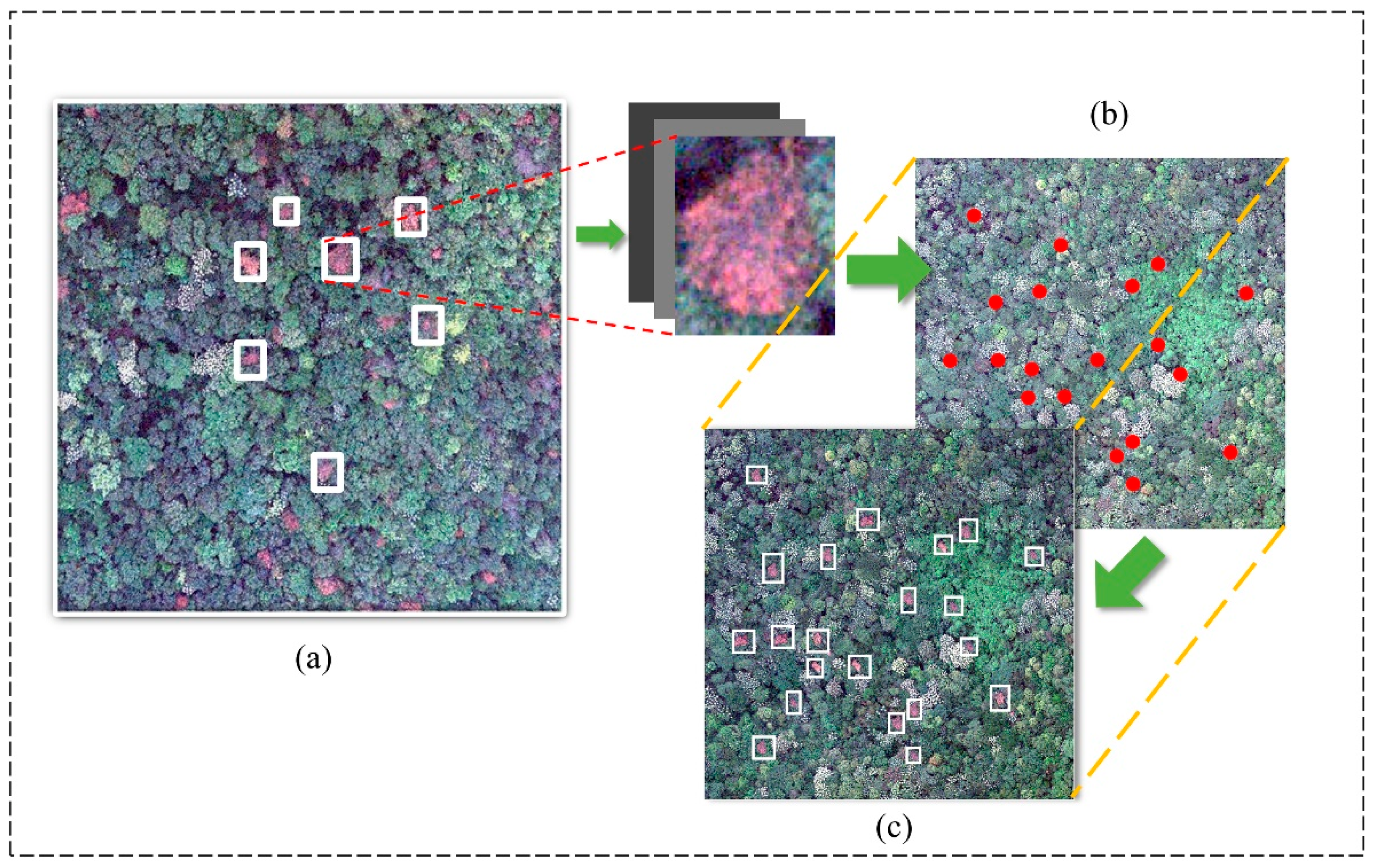
2.2.2. Augmentation Strategy for Small-SDT Detection

There are two issues in SDT detection concerning the dataset we derived. First, due to the small shape (<32 × 32 pixels) of the Pinus tree crowns and the low number of dead trees in an area, the samples of dead tree crowns were not enough and the area covered by dead tree crowns was much smaller in each image, which indicated a lack of diversity in the locations of SDT trees. Second, in terms of number, the SDTs in each input image are not distributed homogenously; the number of SDTs ranged from 10 to 200 in each input image. This phenomenon caused a distribution imbalance problem. In order to overcome these problems, we adopted an augmentation strategy called the adaptive oversampling and allocating (AOA) method to augment samples based on the research of Kisantal (2019) [28]. The main idea of AOA is to oversample a certain small object and allocate it to each input image by copy–pasting according to a priori information of small-object distribution. The total number of oversampled small objects n can be calculated by:

$$n=min\left\{\theta n_0,\eta \frac{A}{\overline{a}}\right\}$$

(3)

where $\theta$ is the oversampling rate, $n_0$ is the initial number of small objects, $\eta$ is the density coefficient to control the maximum number of oversampled objects, the initial value was set to 5%, $A$ is the total area of images, and $\overline{ a}$ is the average area of small objects.

Then, the allocation strategy was used to allocate the oversampled number to each input image with the following equation:

$$n_i=n\times \frac{e^{\left(-\alpha \left(r_i-\overline{r}\right)\right)}}{{{\displaystyle \sum }}_i{e}^{\left(-\alpha \left(r_i-\overline{r}\right)\right)}}$$

(4)

where $n_i$ is the oversampled number in the ith input image, $\alpha$ is the adjusted coefficient, $r_i$ is the ratio of the initial number of small objects of the ith image to the total number of small objects in all images, $\overline{r}$ is the averaged sample ratio of all input images.

Lastly, we randomly selected $n_i$ SDTs objects in images and cropped out a small square image from each image and pasted them in random locations of images without diseased pine area (Figure 3). When pasting each object, we ensured that the pasted object did not overlap with any existing objects and the pasted areas were in the disease-free areas with the same forest type as the samples. The aim was to simulate the distribution diversity of diseased wood in real scenarios.

2.2.3. Multi-Scale Spatial Supervision Convolutional Network

A multi-scale spatial supervision convolutional network architecture (MSSCN) was proposed in our study to detect the SDTs in a complex background. The architecture of MSSCN was seen in Figure 4. This model was based on a fully convolutional network (FCN) [32], the main structure includes the encoder stage and the decoder stage.

The encoder stage is a downsampling process to derive multi-scale spatial features and contains five convolutional blocks (Figure 4). The first block has one convolutional layer with 64 filters of size 3 × 3, followed by a 2 × 2 max-pooling layer. The second bock has three convolutional layers with 128 filters of size 3 × 3 followed by a 2 × 2 max-pooling layer. The third block has four convolutional layers with 128 filters of size 3 × 3 filters followed by a 2 × 2 max-pooling layer. The fourth block has six convolutional layers with 128 filters of size 3 × 3 followed by a 2 × 2 max-pooling layer. The fifth block has six convolutional layers with 128 filters of size 3 × 3 followed by a 2 × 2 max-pooling layer. All convolutional layers use rectified linear units (ReLU) as the activation function.

The difference from the conventional Resnet34 is that we add the atrous block in the last four convolutional blocks, which aims to solve the problem of lost spatial information of a single plant disease in the downsampling process and proposes an attention mechanism to extract the spatial details of the SDTs.

Actually, an atrous block is the aggregation of a series of dilated convolutional layers combined with a 1 × 1 convolutional layer and a sigmoid layer (Figure 4). It allows us to effectively enlarge the field of view of filters without increasing the number of parameters or the amount of computation and to extract spatial-pyramid-feature information [33].

Considering 2D processing, for each dilated convolutional layer, it can be described as an equation:

$$y\left(i,j\right)={\displaystyle \sum }_{p=0}^{k-1}{{\displaystyle \sum }}_{q=0}^{k-1}x\left(i+m\times p,j+m\times q\right)w\left(p,q\right)$$

(5)

where $x$ represents the input feature map; $y$ is the output feature map; $i$, $j$ represent the row and column in the input and output feature map; $w$ is the kernel filter with $k$×$k$ size; $p$ and $q$ are the positions in $w$; and $m$ is the dilation rate which represents the stride in the input feature map and helps to enlarge the field of view of kernel filter. Dilation can increase the receptive field of a convolution kernel. The field view size of a dilated convolutional layer with dilation rate $m$ and kernel size $k$ can be computed as Equation (6).

$$FOV=\left(m-1\right)\times \left(k-1\right)+k$$

(6)

With different $m$, we can derive serious receptive field information. In our study, an atrous block is constructed with a dilation rate of 3, 6, 12, and 18 followed by a 1 × 1 conventional layer and a sigmoid layer. This atrous block was added to the initial structure (Figure 4), which provides supervision weight for shallow and middle layer features, and guides the model to pay more attention to spatial and contextual information.

In the decoder stage, an upsampling convolutional layer was used to expand the size of low-level features and derive the same resolution with input features at the last step. Moreover, a concatenation with the corresponding feature map in the encoder stage was used to compensate for the lost information in the max-pooling layer and enable precise localization [32].

To train this MSSCN model, the mean square error (MSE) loss function was applied at the end of the model. The formula can be seen in Equation (7).

$$MSE=\sum {(y-f_{\theta }(x))}^2$$

(7)

where $y$ represents the ground confidence map; $f_{\theta }\left(x\right)$ represents the predicted value of the model.

2.2.4. SDT Localization from the Confidence Map

The location of each standing dead tree is derived from the peaks (local maximum) of the predicted confidence map. First, the peaks must have confidence values greater than a threshold T. Second, the peaks need to be separated by at least δ pixels to avoid the noise and prevent the SDTs very close to each other from being detected as one item. In our study, we set the T as 0.5 and δ as 10 pixels.

2.2.5. Experiment Setup

The original images in sites A and B were subset to 256 × 256 pixels patches. The patches in site A were used to test the model performance and the patches in site B were used to train our MSSCN model. In the end, we acquired 566 training patches and 139 test patches. Since the number of diseased trees was small and not uniform in the training patches, we tested the influence of the oversampling rate on the detection accuracy using our model; the oversampling rate $\theta$ was set from 1.0 to 2.0 with steps of 0.2 (Equation (3)). The crop window size was set according to the crown size of trees and the image spatial resolution; we set it to 20 pixels based on the average crown size in our study. This ensures the distribution of pasted dead tree crowns in the whole map is rational and does not cause too much concentration of SDTs.

In order to test the performance of the MSSCN model, a benchmark comparison was provided by a standard fully convolutional network model (FCN), such as FCN8s and U-Net.

In model training, the stochastic gradient descent (SGD) optimizer was used with a momentum of 0.9. The hyperparameter of the learning rate and the number of epochs was tuned. In our study, they were set to 0.01 and 100.

2.2.6. Assessment of Model Accuracy

For quantitative evaluation of the model performance, we formed the confusion matrix and derived precision (P), recall (R), and F1-score (F1) to assess the accuracy. The equations are listed as follows.

$$P=\frac{TP}{TP+FP}$$

(8)

$$R=\frac{TP}{TP+FN}$$

(9)

$$F1=2\times \frac{P\times R}{P+R}$$

(10)

Here, R (recall) is the tree detection rate, P (precision) is the correctness of the detected trees, F1 is the overall accuracy of the detected trees, TP (true positive) is the number of correctly detected trees, FN (false negative) is the number of trees that were not detected (omission error), and FP (false positive) is the number of extra trees that did not exist in the field (commission error).

3. Results

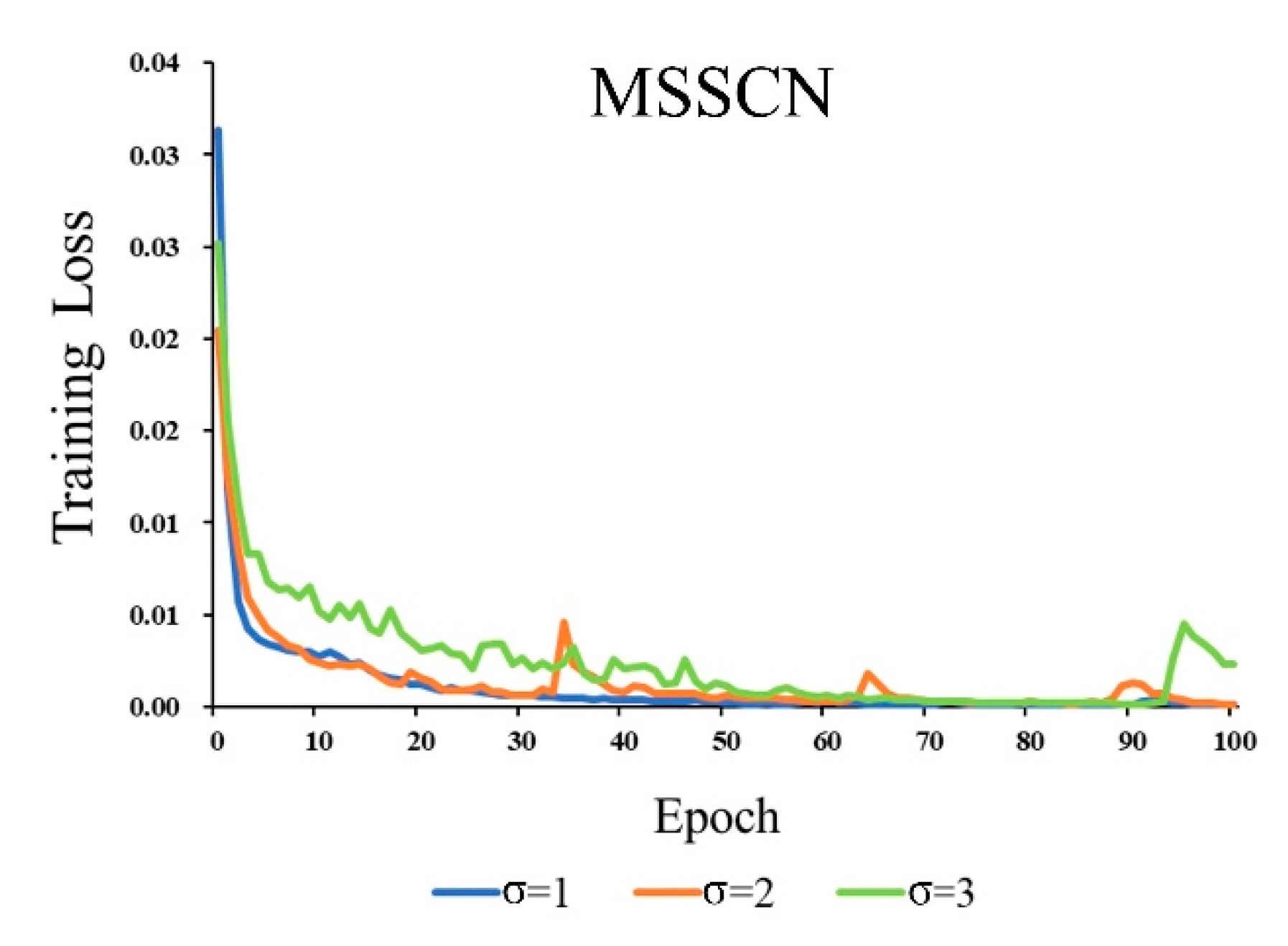
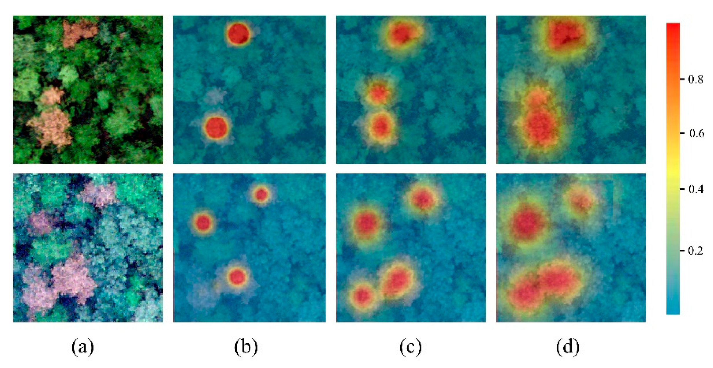
3.1. Analysis of Gaussian Kernel Parameter

Figure 5 presents the relationship between loss values with epochs at different Gaussian kernel parameters. The purpose of this test was to show how much the Gaussian kernel parameter $\sigma$ influences the results with the MSSCN model. In accordance with the tree crown size, we tested $\sigma$ increases from 1 to 3 with steps of 1. The results show that $\sigma$ had a great influence on the results. In our models, the training and validation loss function values were more stable in small $\sigma$ than in large $\sigma$ as $\sigma$ influenced the confidence map, whether the tree canopy was a proper cover or not. When using small $\sigma$, the areas around the peak points in the confidence map were smaller than the tree canopy, and isolated treetops can clearly be found (Figure 6a,b). In contrast, when using the bigger $\sigma$, the areas around peaks may be confused when the peaks are close; individual trees cannot be clearly distinguished at the boundary area (Figure 6d).

The accuracy with different $\sigma$ in our research area is listed in

Table 3. The evaluated $\sigma$ on generating the confidence map to train with the MSSCN model.

$\mathit{\sigma }$	Precision	Recall	F1-Score
1.0	0.95	0.62	0.74
2.0	0.92	0.69	0.79
3.0	0.83	0.62	0.71

. The best result was obtained for $\sigma$ = 2.0, which is better fitted to the size of the tree canopy in this case.

3.2. Analysis of Oversampling Method

Figure 7 presents the detection accuracy metrics in precision, recall, and F1 values changed with the oversampling rate $\theta$ when σ is set to 2.0.

In general, we found that the oversampling strategy had a positive effect on overall accuracy. From Figure 7, we found that, with an increase in $\theta$, recall and F1 values increased compared to the original training size ($\theta$ = 1), while the precision value was higher than 98.8% and did not change much when $\theta$ increased. The most gain was achieved when $\theta$ was set to 1.6, which help to improve the recall value by 0.84 and F1 value by 0.89. While $\theta$ is greater than 1.6, the growth rate of recall and F1 value decreased but is still greater than the original.

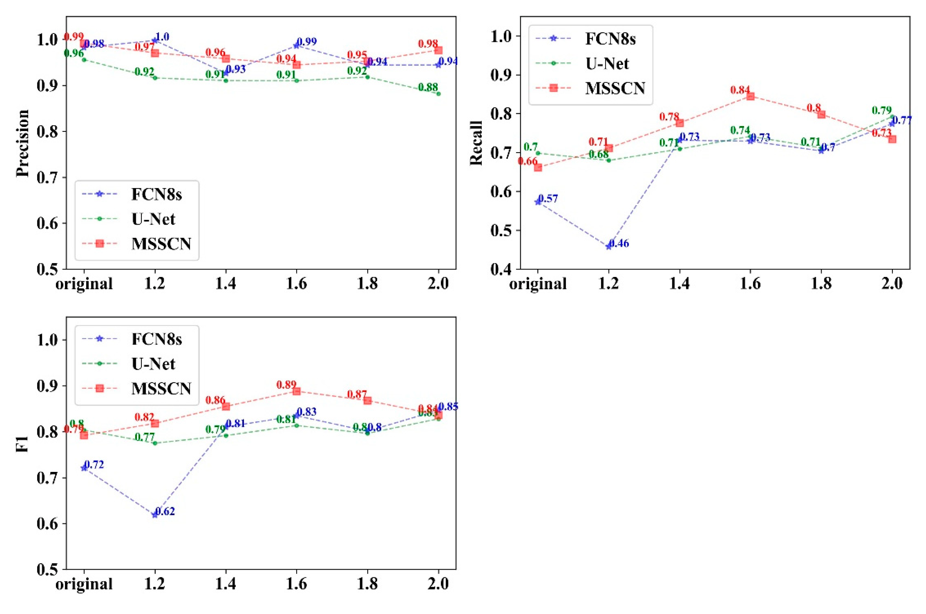
3.3. Comparison of the Accuracy of Different Models

The proposed method was compared with recent benchmark methods such as FCN8s and U-Net.

Table 4. The comparison of the proposed approach with benchmark approaches in different sites. Recall below 0.7 is colored light gray, while F1 over 0.85 is marked with dark gray.

Model	Site	TP	FN	FP	P	R	F1
FCN8s	A-1	99	17	2	0.98	0.85	0.91
	A-2	71	47	0	1.00	0.60	0.75
	A-3	45	22	1	0.98	0.67	0.80
	A-4	313	83	4	0.99	0.79	0.88
Avg					0.99	0.73	0.83
U-Net	A-1	100	16	8	0.93	0.86	0.89
	A-2	70	48	5	0.93	0.59	0.73
	A-3	51	16	6	0.89	0.76	0.82
	A-4	297	99	38	0.89	0.75	0.81
Avg					0.91	0.74	0.81
MSSCN	A-1	104	12	11	0.90	0.90	0.90
	A-2	84	34	0	1.00	0.71	0.83
	A-3	62	5	5	0.93	0.93	0.93
	A-4	335	61	18	0.95	0.85	0.89
Avg					0.94	0.84	0.89

shows the results obtained by all methods using precision, recall, and F1 metrics across four different testing sites with oversampling rate θ set to 1.6 and Gaussian kernel parameter σ set to 2.

We can see that the proposed method MSSCN achieved the best results in F1 and recall metrics with averages of 0.89, and 0.84 across all test sites, respectively. In addition, the MSSCN method achieved a precision of 0.94, while FCN8s and U-Net provided averaged precision values of 0.99 and 0.89, respectively.

We also found a notable difference in accuracy at different testing sites. In general, a better result (highest F1, recall, and precision) will be obtained in pure masson forests with low dead-tree intensity than in mixed forests with high dead-tree intensity.

In addition, the precision of all methods was larger than the recall in all testing sites. The differences between precision and recall were also larger with benchmark methods (FCN8s, U-Net) than the MSSCN method, which means that our proposed method was not insensitive to different forest types and disease intensity outbreak areas.

Figure 8 shows the visual results of predictions generated by three methods in different PWD intensity sites. We can see that our approach has fewer errors in detecting dead trees, while FCN8s and U-Net approaches omit dead trees, especially in mixed forests with high intensity.

4. Discussion

4.1. The Effect of the Gaussian Kernel Function

The Gaussian kernel function helped us to easily conduct “soft annotation” concerning the training samples. Prior studies [24,31,34], have noted that it was laborious work to depict dead tree crown boundaries as training samples, while in our study we only collected the center position to represent diseased wood and used the Gaussian kernel function to simulate the spatial distribution probability map (called confidence map) to represent the diseased area. This “soft annotation” method not only reduces the annotation workloads but also quantitively describes the confidence probability of the diseased individual tree crown and surrounding elements.

However, not much attention was paid in the previous study to the effect of the Gaussian kernel parameter $\sigma$ on results. In our study, we found that the value of σ directly affected the confidence map. A larger $\sigma$ resulted in a larger high-probability area in the confidence map, which would result in a higher weight to the background pixels than the target pixels in the MSSCN model and decreased training accuracy in the end. Especially in the complex stands, due to the small tree crown with canopy gap, it is difficult to obtain suitable data in this complex forest area (Figure 6). Determining how to obtain an appropriate $\sigma$ in the monitoring area is important for accurately detecting dead trees [35]. In this study, we tested three Gaussian parameters and found that the relatively small Gaussian filtering range is better than others. In the future, we should build a strategy to obtain a $\sigma$ with a self-adaption method according to the forest stand condition.

4.2. Oversampling Strategy in Promoting Detection Accuracy

One of the factors behind the low accuracy in object detection is the lack of representation of objects in training data, especially in small-object detection and imbalance samples [36]. In our study, the crown size of a standing dead tree was diverse and the training number in each image scene varied widely due to the forest type and PWD outbreak intensity. Imbalance of samples and tree crown size in each training image was very common. Oversampling and augmentation are very common strategies for resolving problems. In accordance with Kisantal (2019), the oversampling strategy with the copy–pasting method was used to provide a variety of spatial distribution states for standing dead trees, which makes the model more generalized and improves the detection accuracy [28]. The parameter called the oversample rate $\theta$ in the copy–pasting method is very important for training because unsuitable $\theta$ may cause overfitting or underfitting in the DL model [37]. In our study, we also found that “the bigger the better” does not apply to the oversample rate. With an increase in $\theta$, the accuracy metrics do not show a linear growth trend. In terms of F1 and recall metrics, the best accuracy with the MSSCN model was achieved when $\theta$ set to 1.6 in our study. In terms of the precision metric, we found that it is independent of $\theta$. These results indicated that our proposed method can predict standing dead trees with high recall and precision, having a very low number of false detection and commission errors. This means that our model can provide a trade-off between the precision and recall concerning detection accuracy. However, in other forest conditions with different input data, the best oversample rate should be carefully determined by the input training samples.

4.3. MSSCN Model on Detection Accuracy

Several reports have shown that fully convolutional neural networks present a remarkable ability in classification and object detection [20]. Meanwhile, these studies also point out that it is a challenging task in detecting multi-scale objects, especially in a complex environment. In our study, we found that the dead-tree crown size and sample number in each image scene were diverse, which leads to the low recall accuracy in FCN8s and U-Net. There are two reasons: one is that FCN8s and U-Net models easily lose spatial information in downsampling, especially when processing high-resolution images [38]; the second reason is that some small tree crowns often contain only a few pixels, which is often ignored in the downsampling process, resulting in the model not being able to restore more positioning reference information in prediction [39,40].

In order to solve this problem, the multi-scale spatial attention module implemented by the atrous conventional block was added to the deep learning network to generate multi-scale features by aggregation of series-dilated convolutional filters at different full convolutional layers [41,42]. This helps us to enlarge the field of view of each filter and find the best trade-off between the context information and the accurate localization [26,33,43]. This mechanism improves the missing detection problem in FCN8s and U-Net model, and increases the recall accuracy of small dead-tree crowns in dense canopy scenes, as shown in Figure 8. Moreover, compared with FCN8s and U-Net model, the multi-scale spatial attention module enables the model to learn the spatial relationship between any position in the feature map, which can highlight the accurate position of the dead trees and reduce the interference of background noise [44].

4.4. The Influence of Forest Type and Disease Outbreak Intensity on Detection Accuracy

Prior studies have noted that the complexity of forest types has an influence on the detection results, especially in individual tree detection [29,35]. We also found that it is easier to detect dead trees in pure forests than in mixed forests in our research area. The main reason is that, due to the diversity of trees in mixed forests, the crown features’ variability in remote-sensing images is magnified, which would cause the model to become more difficult to train. This finding is consistent with that of Chadwick (2020), who suggested that accurate tree detection is possible with fine-spatial-resolution imagery and point clouds [45].

Moreover, we also found disease outbreak intensity in the research area has an effect on detection accuracy. The main possible reason is a higher diversity of canopy characteristics in the remote-sensing images caused by the different stages of pest occurrence. From Figure 8, we can obviously find diverse colors in canopy colors from dark green to dark red in high-disease-infestation areas. In addition, the canopy structure may also be influenced by the different levels of disease infestation. The variety of canopy color and structure in high-disease-outbreak areas caused the model to become more difficult to train than the low-intensity area. Many researchers have found that the stage of pest or disease outbreak influenced the tree mortality mapping with high-spatial-resolution satellite imagery [46]. Complex color variations of the canopy at different disease stages further increase the difficulty of SDT detection when training samples are imbalanced. Further research should be undertaken to investigate the characteristics of the canopy at different disease stages.

5. Conclusions

Comprehensive, rapid, and accurate identification of pine nematode diseased trees in a complex forest environment is basic and challenging work. In this study, we proposed a novel method called the MSSCN model, which combines the Gaussian filter and multi-scale spatial attention to detect standing dead trees in different forest types and disease-outbreak-intensity areas. In addition, the oversample strategy called the copy–pasting method was used to solve the problem of lack of efficient samples. Validation at four different forest areas belonging to two forest types and two diseased outbreak intensities showed that (1) the copy–pasting method can help to improve the detection accuracy, but the best oversample rate should be carefully determined by the input training samples and image data. (2) Based on the two-dimensional spatial Gaussian kernel distribution function and the multi-scale spatial attention structure, the MSSCN model can effectively find the dead-tree extent in a confidence map; when this is followed by maximum location searching, we can easily locate the individual dead trees. The averaged precision, recall, and F1-score across different forest types and disease-outbreak-intensity areas can achieve 0.94, 0.84, and 0.89, respectively, which is the best performance among FCN8s and U-Net. (3) In terms of forest type and outbreak intensity, the MSSCN performs best in pure pine forest type and low-outbreak-intensity areas. Compared with FCN8s and U-Net, the MSSCN can achieve the best recall accuracy in all forest types and outbreak-intensity areas. Meanwhile, the precision metric is also maintained at a high level, which means that the proposed method provides a trade-off between the precision and recall concerning detection accuracy.

References

1. Tóth, Á. Bursaphelenchus Xylophilus, the Pinewood Nematode: Its Significance and a Historical Review. Acta Biol. Szeged. 2011, 55, 213–217. [Google Scholar]
2. Carnegie, A.J.; Venn, T.; Lawson, S.; Nagel, M.; Wardlaw, T.; Cameron, N.; Last, I. An Analysis of Pest Risk and Potential Economic Impact of Pine Wilt Disease to Pinus Plantations in Australia. Aust. For. 2018, 81, 24–36. [Google Scholar] [CrossRef]
3. Zhao, J.; Huang, J.; Yan, J.; Fang, G. Economic Loss of Pine Wood Nematode Disease in Mainland China from 1998 to 2017. Forests 2020, 11, 1042. [Google Scholar] [CrossRef]
4. Cha, D.; Kim, D.; Choi, W.; Park, S.; Han, H. Point-of-care diagnostic (POCD) method for detecting Bursaphelenchus xylophilus in pinewood using recombinase polymerase amplification (RPA) with the portable optical isothermal device (POID). PLoS ONE 2020, 15, e0227476. [Google Scholar] [CrossRef] [PubMed] [Green Version]
5. Abdulridha, J.; Ehsani, R.; Abd-Elrahman, A.; Ampatzidis, Y. A Remote Sensing Technique for Detecting Laurel Wilt Disease in Avocado in Presence of Other Biotic and Abiotic Stresses. Comput. Electron. Agric. 2019, 156, 549–557. [Google Scholar] [CrossRef]
6. Proença, D.N.; Grass, G.; Morais, P.V. Understanding pine wilt disease: Roles of the pine endophytic bacteria and of the bacteria carried by the disease-causing pinewood nematode. MicrobiologyOpen 2017, 6, e00415. [Google Scholar] [CrossRef] [PubMed]
7. Stone, C.; Mohammed, C. Application of Remote Sensing Technologies for Assessing Planted Forests Damaged by Insect Pests and Fungal Pathogens: A Review. Curr. For. Rep. 2017, 3, 75–92. [Google Scholar] [CrossRef]
8. Kang, J.S.; Kim, A.-Y.; Han, H.R.; Moon, Y.S.; Koh, Y.H. Development of Two Alternative Loop-Mediated Isothermal Amplification Tools for Detecting Pathogenic Pine Wood Nematodes. For. Pathol. 2015, 45, 127–133. [Google Scholar] [CrossRef]
9. Li, X.; Tong, T.; Luo, T.; Wang, J.; Rao, Y.; Li, L.; Jin, D.; Wu, D.; Huang, H. Retrieving the Infected Area of Pine Wilt Disease-Disturbed Pine Forests from Medium-Resolution Satellite Images Using the Stochastic Radiative Transfer Theory. Remote Sens. 2022, 14, 1526. [Google Scholar] [CrossRef]
10. Zhang, Y.; Dian, Y.; Zhou, J.; Peng, S.; Hu, Y.; Hu, L.; Han, Z.; Fang, X.; Cui, H. Characterizing Spatial Patterns of Pine Wood Nematode Outbreaks in Subtropical Zone in China. Remote Sens. 2021, 13, 4682. [Google Scholar] [CrossRef]
11. Zhang, B.; Ye, H.; Lu, W.; Huang, W.; Wu, B.; Hao, Z.; Sun, H. A Spatiotemporal Change Detection Method for Monitoring Pine Wilt Disease in a Complex Landscape Using High-Resolution Remote Sensing Imagery. Remote Sens. 2021, 13, 2083. [Google Scholar] [CrossRef]
12. Hart, S.J.; Veblen, T.T. Detection of Spruce Beetle-Induced Tree Mortality Using High- and Medium-Resolution Remotely Sensed Imagery. Remote Sens. Environ. 2015, 168, 134–145. [Google Scholar] [CrossRef] [Green Version]
13. Guo, Q.; Kelly, M.; Gong, P.; Liu, D. An Object-Based Classification Approach in Mapping Tree Mortality Using High Spatial Resolution Imagery. GIScience Remote Sens. 2007, 44, 24–47. [Google Scholar] [CrossRef]
14. Iordache, M.-D.; Mantas, V.; Baltazar, E.; Pauly, K.; Lewyckyj, N. A Machine Learning Approach to Detecting Pine Wilt Disease Using Airborne Spectral Imagery. Remote Sens. 2020, 12, 2280. [Google Scholar] [CrossRef]
15. Meddens, A.J.H.; Hicke, J.A.; Vierling, L.A.; Hudak, A.T. Evaluating Methods to Detect Bark Beetle-Caused Tree Mortality Using Single-Date and Multi-Date Landsat Imagery. Remote Sens. Environ. 2013, 132, 49–58. [Google Scholar] [CrossRef]
16. Skakun, R.S.; Wulder, M.A.; Franklin, S.E. Sensitivity of the Thematic Mapper Enhanced Wetness Difference Index to Detect Mountain Pine Beetle Red-Attack Damage. Remote Sens. Environ. 2003, 86, 433–443. [Google Scholar] [CrossRef]
17. Fassnacht, F.E.; Latifi, H.; Ghosh, A.; Joshi, P.K.; Koch, B. Assessing the Potential of Hyperspectral Imagery to Map Bark Beetle-Induced Tree Mortality. Remote Sens. Environ. 2014, 140, 533–548. [Google Scholar] [CrossRef]
18. Hall, R.J.; Castilla, G.; White, J.C.; Cooke, B.J.; Skakun, R.S. Remote Sensing of Forest Pest Damage: A Review and Lessons Learned from a Canadian Perspective. Can. Entomol. 2016, 148, S296–S356. [Google Scholar] [CrossRef]
19. Wulder, M.A.; White, J.C.; Carroll, A.L.; Coops, N.C. Challenges for the Operational Detection of Mountain Pine Beetle Green Attack with Remote Sensing. For. Chron. 2009, 85, 32–38. [Google Scholar] [CrossRef] [Green Version]
20. Hicke, J.A.; Logan, J. Mapping Whitebark Pine Mortality Caused by a Mountain Pine Beetle Outbreak with High Spatial Resolution Satellite Imagery. Int. J. Remote Sens. 2009, 30, 4427–4441. [Google Scholar] [CrossRef]
21. Coops, N.C.; Johnson, M.; Wulder, M.A.; White, J.C. Assessment of QuickBird High Spatial Resolution Imagery to Detect Red Attack Damage Due to Mountain Pine Beetle Infestation. Remote Sens. Environ. 2006, 103, 67–80. [Google Scholar] [CrossRef]
22. Oumar, Z.; Mutanga, O. Using WorldView-2 Bands and Indices to Predict Bronze Bug (Thaumastocoris Peregrinus) Damage in Plantation Forests. Int. J. Remote Sens. 2013, 34, 2236–2249. [Google Scholar] [CrossRef]
23. Fassnacht, F.E.; Latifi, H.; Stereńczak, K.; Modzelewska, A.; Lefsky, M.; Waser, L.T.; Straub, C.; Ghosh, A. Review of Studies on Tree Species Classification from Remotely Sensed Data. Remote Sens. Environ. 2016, 186, 64–87. [Google Scholar] [CrossRef]
24. Qiao, R.; Ghodsi, A.; Wu, H.; Chang, Y.; Wang, C. Simple Weakly Supervised Deep Learning Pipeline for Detecting Individual Red-Attacked Trees in VHR Remote Sensing Images. Remote Sens. Lett. 2020, 11, 650–658. [Google Scholar] [CrossRef]
25. Xiao, C.; Qin, R.; Huang, X.; Li, J. A study of using fully convolutional network for treetop detection on remote sensing data. ISPRS Ann. Photogramm. Remote Sens. Spat. Inf. Sci. 2018, IV–1, 163–169. [Google Scholar]
26. Qin, J.; Wang, B.; Wu, Y.; Lu, Q.; Zhu, H. Identifying Pine Wood Nematode Disease Using Uav Images and Deep Learning Algorithms. Remote Sens. 2021, 13, 162. [Google Scholar] [CrossRef]
27. Buda, M.; Maki, A.; Mazurowski, M.A. A Systematic Study of the Class Imbalance Problem in Convolutional Neural Networks. Neural Netw. 2018, 106, 249–259. [Google Scholar] [CrossRef] [PubMed] [Green Version]
28. Kisantal, M.; Wojna, Z.; Murawski, J.; Naruniec, J.; Cho, K. Augmentation for small object detection. arXiv 2019, arXiv:1902.07296. [Google Scholar]
29. Lopatin, J.; Dolos, K.; Kattenborn, T.; Fassnacht, F.E. How Canopy Shadow Affects Invasive Plant Species Classification in High Spatial Resolution Remote Sensing. Remote Sens. Ecol. Conserv. 2019, 5, 302–317. [Google Scholar] [CrossRef]
30. Liu, X.; Frey, J.; Denter, M.; Zielewska-Büttner, K.; Still, N.; Koch, B. Mapping Standing Dead Trees in Temperate Montane Forests Using a Pixel- and Object-Based Image Fusion Method and Stereo WorldView-3 Imagery. Ecol. Indic. 2021, 133, 108438. [Google Scholar] [CrossRef]
31. Osco, L.P.; de Arruda, M.D.S.; Marcato Junior, J.; da Silva, N.B.; Ramos, A.P.M.; Moryia, É.A.S.; Imai, N.N.; Pereira, D.R.; Creste, J.E.; Matsubara, E.T.; et al. A Convolutional Neural Network Approach for Counting and Geolocating Citrus-Trees in UAV Multispectral Imagery. ISPRS J. Photogramm. Remote Sens. 2020, 160, 97–106. [Google Scholar] [CrossRef]
32. Long, J.; Shelhamer, E.; Darrell, T. Fully convolutional networks for semantic segmentation. In Proceedings of the IEEE Conference on Computer Vision and Pattern Recognition (CVPR), Boston, MA, USA, 7–12 June 2015; pp. 3431–3440. [Google Scholar] [CrossRef] [Green Version]
33. Chen, L.-C.; Papandreou, G.; Kokkinos, I.; Murphy, K.; Yuille, A.L. DeepLab: Semantic Image Segmentation with Deep Convolutional Nets, Atrous Convolution, and Fully Connected CRFs. IEEE Trans. Pattern Anal. Mach. Intell. 2018, 40, 834–848. [Google Scholar] [CrossRef] [PubMed] [Green Version]
34. Pfister, T.; Charles, J.; Zisserman, A. Flowing Convnets for Human Pose Estimation in Videos. In Proceedings of the IEEE international conference on computer vision, Santiago, Chile, 7–13 December 2015; pp. 1913–1921. [Google Scholar]
35. Yun, T.; Jiang, K.; Li, G.; Eichhorn, M.P.; Fan, J.; Liu, F.; Chen, B.; An, F.; Cao, L. Individual Tree Crown Segmentation from Airborne LiDAR Data Using a Novel Gaussian Filter and Energy Function Minimization-Based Approach. Remote Sens. Environ. 2021, 256, 112307. [Google Scholar] [CrossRef]
36. White, J.C.; Wulder, M.A.; Brooks, D.; Reich, R.; Wheate, R.D. Detection of Red Attack Stage Mountain Pine Beetle Infestation with High Spatial Resolution Satellite Imagery. Remote Sens. Environ. 2005, 96, 340–351. [Google Scholar] [CrossRef]
37. Mai, Z.; Hu, X.; Peng, S.; Wei, Y. Human Pose Estimation via Multi-Scale Intermediate Supervision Convolution Network. In Proceedings of the 2019 12th International Congress on Image and Signal Processing, BioMedical Engineering and Informatics (CISP-BMEI), Suzhou, China, 19–21 October 2019; IEEE: Suzhou, China, 2019; pp. 1–6. [Google Scholar]
38. Han, Z.; Dian, Y.; Xia, H.; Zhou, J.; Jian, Y.; Yao, C.; Wang, X.; Li, Y. Comparing Fully Deep Convolutional Neural Networks for Land Cover Classification with High-Spatial-Resolution Gaofen-2 Images. ISPRS Int. J. Geo-Inf. 2020, 9, 478. [Google Scholar] [CrossRef]
39. Simonyan, K.; Zisserman, A. Very Deep Convolutional Networks for Large-Scale Image Recognition. In Proceedings of the 3rd International Conference on Learning Representations, ICLR 2015—Conference Track Proceedings, San Diego, CA, USA, 7–9 May 2015; pp. 1–14. [Google Scholar]
40. He, K.; Zhang, X.; Ren, S.; Sun, J. Deep Residual Learning for Image Recognition. In Proceedings of the IEEE conference on computer vision and pattern Recognition (CVPR), Las Vegas, NV, USA, 27–30 June 2016; pp. 770–778. [Google Scholar]
41. Yu, F.; Koltun, V.; Funkhouser, T. Dilated Residual Networks. In Proceedings of the Proceedings, 30th IEEE Conference on Computer Vision and Pattern Recognition (CVPR), Honolulu, HI, USA, 21–26 July 2017; pp. 636–644. [Google Scholar]
42. Chen, L.-C.; Papandreou, G.; Schroff, F.; Adam, H. Rethinking Atrous Convolution for Semantic Image Segmentation. arXiv 2017, arXiv:1706.05587. [Google Scholar]
43. Woo, S.; Park, J.; Lee, J.Y.; Kweon, I.S. CBAM: Convolutional Block Attention Module. arXiv 2018, arXiv:1807.06521. [Google Scholar]
44. Li, X.; Xu, F.; Lyu, X.; Gao, H.; Tong, Y.; Cai, S.; Li, S.; Liu, D. Dual Attention Deep Fusion Semantic Segmentation Networks of Large-Scale Satellite Remote-Sensing Images. Int. J. Remote Sens. 2021, 42, 3583–3610. [Google Scholar] [CrossRef]
45. Chadwick, A.J.; Goodbody, T.R.H.; Coops, N.C.; Hervieux, A.; Bater, C.W.; Martens, L.A.; White, B.; Röeser, D. Automatic Delineation and Height Measurement of Regenerating Conifer Crowns under Leaf-off Conditions Using UAV Imagery. Remote Sens. 2020, 12, 4104. [Google Scholar] [CrossRef]
46. Meddens, A.J.H.; Hicke, J.A. Spatial and Temporal Patterns of Landsat-Based Detection of Tree Mortality Caused by a Mountain Pine Beetle Outbreak in Colorado, USA. For. Ecol. Manag. 2014, 322, 78–88. [Google Scholar] [CrossRef]
Figure 1. Localization of the study areas (A and B). Training and testing areas are labeled with different colors (blue for training and red for testing).
Remotesensing 14 03075 g001
Figure 2. Gaussian kernel function distribution diagram.
Remotesensing 14 03075 g002
Figure 3. Schematic diagram of the data enhancement process. (a) Crop out the SDTs with adapted pixel size window from each image without overlap; (b) pasted at random without overlap; (c) locations in the pasted area in non-diseased pine area.
Remotesensing 14 03075 g003
Figure 4. The architecture of the multi-scale spatial supervision convolution network.
Remotesensing 14 03075 g004
Figure 5. Training loss of the MSSCN at different Gaussian kernel parameters.
Remotesensing 14 03075 g005
Figure 6. Confidence map generated with different σ values. (a) Ground truth of SDTs; (b) The confidence map when σ is 1; (c) The confidence map when σ is 2; (d) The confidence map when σ is 3.
Remotesensing 14 03075 g006
Figure 7. The comparison of the proposed approach with benchmark approaches in all sites changed with θ when σ was set to 2.
Remotesensing 14 03075 g007
Figure 8. Location results of different approaches in test sites (A-1, A-2, A-3, A-4). TP (true positive) is the number of correctly detected trees, FN (false negative) is the number of trees that were not detected (omission error), and FP (false positive) is the number of extra trees that did not exist in the field (commission error).
Remotesensing 14 03075 g008