Abstract
With the rapid development of global navigation satellite systems (GNSS) and their increasingly wide range of applications in atmospheric science, total electron content (TEC) data are widely used in the theoretical study of layer coupling related to seismicity. This study detected and analyzed pre-earthquake ionospheric anomalies (PEIA) by using TEC data from the Royal Observatory of Belgium (ROB), and analyzed coseismic ionospheric disturbance (CID) with vertical TEC (VTEC) from the GPS stations in earthquake preparation areas. The results show that PEIA appear to increase continuously from 08:00–12:00 UT in the 3 days before a seismic swarm of Mw > 5.0. The ionosphere over the seismogenic zones exhibited large-scale anomalies when multiple seismogenic zones of the Balkan Peninsula spatially and temporally overlapped. Moreover, the TEC around the earthquake centers showed a positive anomaly lasting for 7 h. In a single seismogenic zone in Greece, the TEC around the earthquake center reached over +3.42 TECu. In addition, the CID observed from GPS stations shows that with the increase in the number of earthquakes, the ionosphere over the seismogenic area is more obviously disturbed, and after three strong earthquakes, TEC suddenly decreased over the seismogenic area and formed a phenomenon similar to an ionospheric hole. We conclude that a lithosphere–atmosphere–ionosphere coupling mechanism existed before the seismic swarm appeared in the Balkan Peninsula. Earthquake-induced VTEC anomalies occurred more frequently within a 3–10 day window before the earthquake. This phenomenon is particularly evident when multiple seismogenic zones overlap spatiotemporally.
1. Introduction
With the development and advancement of space exploration technology, researchers have paid increasing attention to seismic ionosphere detection and lithosphere–ionosphere coupling. However, earthquake prediction has been in the exploratory stage because of the complexities behind the causes of earthquakes. There are many reports regarding pre-earthquake geological structural changes and other pre-earthquake anomalies related to earthquakes; among these, the pre-earthquake ionospheric anomaly is a popular topic of contemporary research [1,2,3].
Davies (1964) first detected abnormal ionospheric disturbances above the epicenter of a 9.2 magnitude Alaskan earthquake [4]. Pulinets (2004) observed anomalies appearing in electron densities of the ionospheric F region a few days before some strong earthquakes through the analysis of GPS TEC and other ionospheric parameters from different dedicated satellites [5]. The preliminary results from the above research show that the energy released during seismogenesis can propagate upward into the Earth’s atmosphere, resulting in ionospheric disturbances. The identification of seismo-ionospheric anomalies was made from the analysis of different GNSS satellite measurements based on different statistical methods. For example, by using GPS TEC, Sanchez (2022) found TEC in the form of traveling ionospheric disturbances (TIDs) within 1 h after the mainshock onset during an earthquake in California [6]. Liu (2001) detected TEC 15 days before an earthquake (Mw 7.7) in Taiwan and found three anomalies that provided empirical evidence of earthquake-executed ionosphere anomalies within five days before the mainshock [7]. Chen (2004) found a significant correlation between anomalies and earthquakes in Taiwan and the anomalous depression of the maximum plasma frequency in the ionospheric F2 layer by analyzing these TEC anomalies [8]. Hobara (2005) found from a dedicated satellite’s mission over a seismogenic zone that an abnormal ionospheric disturbance appeared during an 8.3 magnitude earthquake in Hachiko [9]. Ryu (2014) discovered earthquake–ionospheric coupling by detecting ionospheric electron density (IED) data in seismic regions accompanied by PEIA; this report suggested the possible coupling of the lithosphere and ionosphere by the integration of TEC [10]. Similarly, Yao (2016) used a singular spectrum analysis of the TEC time series around the epicenter of the Nepal earthquake and showed positive ionospheric anomalies in the epicenter region before the earthquake [11]. Shah (2020) used global TEC observation data to study ionospheric anomalies before and after earthquakes at different latitudes, and found there were pre-earthquake disturbances and coseismic responses in the temporal and spatial distribution of the TEC data [12]. Tariq (2021) studied the ionospheric anomalies before earthquakes in Pakistan and Islamabad, and the results showed positive anomalies in the ionosphere ten days before the two earthquakes [13]. In general, seismo-ionospheric anomalies appear either a few days to two weeks before large earthquakes or around the earthquake time [14]. Various kinds of great earthquake precursors have been reported so far, but there are few studies on the impact of the seismic swarm on the ionosphere. Therefore, this paper comprehensively describes the ionospheric disturbances of the Balkan–Greece seismic swarm with a case study of both the co- and pre-seismic ionospheric disturbances of the seismic swarm.
2. Experimental Data
To avoid the interference of magnetic storms, earthquakes that occurred under geomagnetic conditions during a quiet period were selected (Kp < 4, F10.7 < 100 and Dst > −30 nT). The Kp and Dst indices were usually lower than 4 and greater than −30 nT, respectively, which indicate that the geomagnetic activity is quiet [15,16]. The seismic data were obtained from the United States Geological Survey (available online: https://earthquake.usgs.gov/earthquakes/search/ (accessed on 10 July 2021)), which provided the reference for calculating the radius of the seismogenic area [11,17]. We also analyzed TEC data from GPS stations operating within the seismogenic zone of the seismic swarm in the Balkan Peninsula (Figure 1). Further details are presented in Table 1.
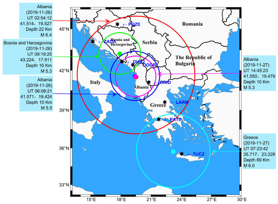
Figure 1.
Geographic map of the locations of seismic swarm in the Balkan Peninsula in 2019. Seismogenic zones are shown by circles. Earthquake information is shown with every epicenter (circular). GPS stations are shown by filled hexagons.

Table 1.
Details of the earthquakes that occurred in the Balkan Peninsula.
We retrieved high-quality TEC data from the ROB by using GPS observations, and the products consist of ionospheric vertical TEC maps over Europe, which were estimated in near real-time every 15 min with 0.5° × 0.5° grids. The maps are available online with a latency of ~3 min in IONEX format at: ftp://gnss.oma.be (accessed on 11 July 2021) and as interactive web pages at: www.gnss.be (accessed on 11 July 2021) [18]. In addition, we calculated the VTEC at seven GPS stations operating within the seismogenic zone of the seismic swarm in the Balkan Peninsula (available online: https://www.epncb.oma.be/ (accessed on 12 July 2021)). The correlation index for the solar activity and geomagnetic activity was obtained from the Goddard Space Flight Center of NASA (available online: https://omniweb.gsfc.nasa.gov/ (accessed on 12 July 2021)).
3. Methods
3.1. Bilinear Interpolation
To determine the TEC of the earthquake center, we used the adjacent four grid points to interpolate the TEC using the bilinear interpolation method. Figure 2 shows the ionospheric grid interpolation diagram.
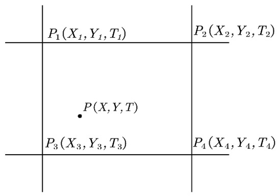
Figure 2.
Schematic diagram of the ionospheric grid interpolation algorithm.
According to the Lagrange interpolant, the ionospheric VTEC value of the interpolation point was obtained. The formula is as follows:
where X and Y are the coordinates of the undetermined interpolation point, the TEC is represented with T, and the grid coordinates are Xi and Yi, respectively.
3.2. Method for PEIA
Because ionospheric variation is affected by many factors, such as solar activity, earth rotation, geomagnetic conditions, and so on, it has a robust diurnal periodicity. The 15-day moving median (MM) method is a quartile-based statistical analysis technique that is used to express the dispersion of data in a powerful statistical technique proposed by Liu [19,20]. This technique is often used to check data anomalies and identify and strengthen periodic signals. Thus, abnormal disturbances in the TEC time series can be extracted using a quartile-based statistical technique. TEC data that were not disturbed by solar activity and geomagnetic anomalies within 15 days before the earthquake were used. The median (Q2), upper (Q1), and lower quartiles (Q3), and the interquartile range (IQR) were calculated. To further improve the reliability of abnormal signals, the constraint method of 1.5 × IQR is adopted [21]. For instance, in order to generate MM, UB and LB for the 16th day, the TEC values for the first 15 days were utilized. Similarly, 15 days of TEC data from between the 2nd and 16th day were used to generate bounds for the 17th day. If more than one-third of the data (e.g., eight hours are anomalous in a day) were greater or lesser than the UBs and LBs in a day, this day was taken as anomalous [20].
where TEC is the median of the first 15 days at the same time, IQR is the quartile of the first 15 days, and equals the IQR multiplied by 1.5 to delimit the upper and lower thresholds. Likewise, TECup and TEClow are the upper and lower confidence limits of the TEC, respectively, and if the observed TEC falls outside of either of the respective bounds, it is declared that a lower or upper abnormal signal is detected, respectively. If the observed value exceeds the upper threshold, a positive disturbance of the TEC is considered. Meanwhile, when the variations in TEC are below the lower bound, it may be a negative PEIA. The TEC exceptions were calculated as follows:
3.3. GNSS TEC Observations and Methods
The TEC from GPS stations operating within the seismogenic zone of the earthquakes was estimated by measuring the phase and amplitude (at a rate of 50 Hz) and code/carrier divergence (at 1 Hz) for each satellite, and the observation interval was 30 s. This calculates the slant TEC (STEC) from the combined frequencies by pseudo-range and carrier-phase measurements using the following equations [22,23]:
where and are carrier phase frequencies of GPS signals at the two ends, P and L represent the pseudo-range and carrier phase observation of the delay path of the GPS signal. , , and are the wavelength of GPS signals, the ambiguity of the ray path, and random residual of the GNSS signal along ray path, while b and d are the instrumental biases of the carrier phase and pseudo-range of the derived signal. Moreover, the STEC was converted into VTEC using the following equation [24]:
where R and H are the radius of the Earth and the height of the top ionospheric layer in atmospheric altitude, respectively. Z is the elevation angle of the satellite for the ionosphere pierce point.
The ionosphere ranges from 60 km to 1000 km above the Earth’s surface; to simplify the ionospheric model, the single-layer ionosphere assumption model is usually introduced. So, in this work, the height of the top layer of the atmospheric altitude was taken as 350 km [25].
4. Analysis and Results
4.1. Geomagnetic Activity Background
The spatial ionospheric variation is closely related to the solar and geomagnetic activity indices [26,27]. Thus, ionospheric anomalies caused by geomagnetism and solar activity should be avoided, and abnormal ionospheric disturbances related to earthquakes were obtained. Figure 3 and Figure 4 show the time series for the F10.7, Dst, and Kp indices from 15 to 29 November 2019. The Dst index does not exceed −30 nT and the Kp index is less than 4, indicating that the geomagnetic field is calm and in a quiet ionospheric period. Therefore, the ionospheric anomalies caused by solar activity and geomagnetic activity can be excluded, and other geophysical signals (e.g., solar and geomagnetic activities) can be distinguished. The data were obtained from NASA’s website at: https://omniweb.gsfc.nasa.gov/ (accessed on 15 July 2021).
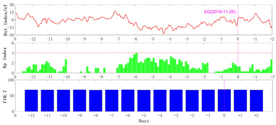
Figure 3.
Changes in F10.7, Dst, and Kp indices from 15 November to 29 November 2019.
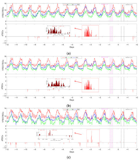
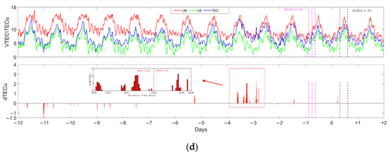
Figure 4.
TEC time series diagram of ionospheric anomalies. The red line represents the lower bound (LB), the green line represents the upper bound (UB), the blue line represents the total electron content (TEC), the vertical dashed lines represent the mainshock, dTECu represents the PEIA. (a) TEC time series of the Albanian earthquake center; (b) TEC time series of earthquake centers in Bosnia and Herzegovina; (c) TEC time series of the central grid of the Greek earthquake; (d) TEC time series of grid points at the confluence of the Greek and Albanian seismogenic regions.
4.2. Time Series Analysis of Epicenter TEC
To observe the affected hours more closely, TEC data were obtained for 15 days at the intersection of the four epicenters and two seismogenic zones, as shown in Figure 4, where the red curve is the upper quartile threshold, the green curve is the lower quartile threshold, the blue curve is the actual TEC value, and the pink and black vertical bars are the earthquake occurrence times. If the TEC data exceeded the upper and lower quartile thresholds, the TEC deviations were drawn on the red histogram at the bottom of the graph. TEC deviations can be seen beyond the upper limits, 3–4 days before successive earthquakes. We observed slight seismo-ionospheric anomalies 10 days before the earthquake. As shown in Figure 4a, at 07:00 UT on 16 November 2019 (10 days before the earthquake), TEC first appeared as a negative anomaly of −0.92 TECu, and at the same time of the next day (17 November), it also appeared and reached −0.93 TECu. Then, the negative anomaly gradually weakened and became a positive anomaly. The positive anomalies were initiated at 08:45 UT on 22 November (4 days before the earthquake), and these positive anomalies, occurred between 08:45 UT on 22 November and 15:45 UT on 23 November (3 days before the earthquake). The maximum time interval of the anomaly was only 1 h. The peak of the positive anomalies appeared at 17:45 UT on 21 November (5 days before the earthquake), and reached 2.54 TECu. The anomalous characteristics of the epicenters of the Bosnia and Herzegovina earthquakes were consistent with those of the Albania earthquake, as shown in Figure 4b. This phenomenon could be explained because the epicenters of the Bosnia and Herzegovina earthquakes were only 137.8 km apart from the epicenter of the Albania earthquake and the two seismogenic zones coincided. However, as shown in Figure 4c, with a single seismogenic zone at the epicenter, there was a negative anomaly of TEC = −2.91 TECu at 23:30 UT on 15 November (11 days before the earthquake), which is similar to the characteristics of the two previous epicenters, while the intensity of the seismo-ionospheric anomalies had no continuity. Then, positive anomalies appeared at 17:30 UT on 22 November (5 days before the earthquake), with the peak at 03:00 UT on 23 November (3 days before the earthquake), and reached 3.42 TECu. Figure 4d shows the seismic ionospheric anomalies in the area where the Albanian seismic zone meets the Greek seismic zone. The positive anomaly characteristics at the intersection of seismogenic zones were very similar to those in the Albania seismogenic zone, with both showing the characteristics of continuous anomalies. Compared with the single earthquake area, the seismic ionospheric anomalies were significantly different. In addition, earthquake-induced VTEC anomalies occurred more frequently within a 3–10-day window with the approach of the earthquake day. The intersection of seismogenic regions resulted in more frequent ionospheric fluctuations. These results suggest that there is a certain correlation between the intersection of seismogenic regions in time and space, and ionospheric disturbance.
4.3. TEC Changes in the Balkan Peninsula Seismic Swarm
In order to study whether CID are caused by various atmospheric waves (Rayleigh surface waves, and internal gravity waves) generated by the seismic swarm, we investigated the TEC responses to the Balkan Peninsula seismic swarm [28,29]. Figure 5 shows the VTEC time series and the trajectory of the ionospheric penetration point (IPP) observed by the GPS station in the earthquake area, where the orbit color matches the color of the observation station. The pentagram on the orbit is the location of the satellite when the earthquake occurs, and the pentagram color corresponds to the color of the earthquake center (when the red earthquake center occurs, it corresponds to the red five-star position on the IPP path, and the blue earthquake center corresponds to the blue five-star). The red arrow is the direction in which the satellite moves.
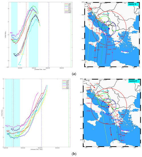
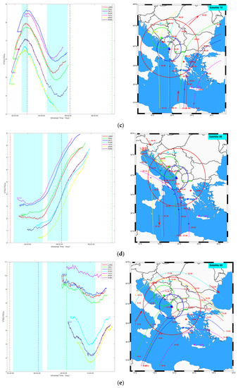
Figure 5.
The left panels present the time series of the original VTEC changes observed by different satellites at different stations and the right panels present the corresponding IPP trajectory of the satellite. Additionally, red, blue and green lines indicate the occurrence of an earthquake in the left figure (the color corresponds to the source in the right figure). The small stars on the track represent the IPP position of the satellite when the earthquake occurs (the color corresponds to the source in the figure) and the red thread indicates the moving direction of the satellite in the right figure. (a) The time series of the original VTEC changes observed by satellite 16 and the IPP trajectory of the satellite. (b) The time series of the original VTEC changes observed by satellite 27 and the IPP trajectory of the satellite. (c) The time series of the original VTEC changes observed by satellite 10 and the IPP trajectory of the satellite. (d) The time series of the original VTEC changes observed by satellite 08 and the IPP trajectory of the satellite. (e) The time series of the original VTEC changes observed by satellite 09 and the IPP trajectory of the satellite.
In the left plane of Figure 5a, we show the VTEC series from 1:00 UT to 5:00 UT recorded by satellite 16 visible from different stations (except for the ZADA station, the IPP longitude range is 11°–13°E) in the seismogenic area. For all stations, CID clearly appear after the earthquake, with time lags of 1–2 h, This phenomenon is consistent with the conclusion of Astafyeva [30,31], and the time needed for acoustic waves to travel from the surface to the IPP. Interestingly, we found that when we compared the VTEC sequence of ZADA station with that of TUC2 station, ZADA station is at the edge of the seismogenic area, IPP also does not pass over the seismogenic area, and the fluctuation amplitude of VTEC sequence is not very obvious. On the contrary, although the TUC2 station is not in the earthquake preparation area, the IPP track is located above the earthquake preparation area and close to the focal center, and it can be clearly seen that it has been strongly disturbed. In addition, it can also be observed that within 2 h before the arrival of the first main earthquake, all stations were disturbed to varying degrees. The perturbation frequency increased as the IPP positions got closer to the source center, with a fluctuation range of 0.1–0.5 TECu, and similar phenomena were observed on other satellites.
The TEC shows rising or falling curvature due to satellite elevation and latitude changes, so it is difficult to observe abnormal conditions. Nevertheless, we observed from the IPP path of satellite 27 (Figure 5b) and satellite 09 (Figure 5e) within 2 h, and its latitude change rate was relatively low. It is obvious that compared with satellite 27 (Figure 5b), when the 6.3 Mw Albanian earthquake struck, CID was observed at all stations on satellite 27. In particular, the ORID station is close to the center of the source, and the IPP is also closest to the center of the source, and its variation in amplitude is large. Figure 5e shows VTEC changes over the seismogenic area after three earthquakes. From the figure on the right, we can see that the IPP of observation satellite 09 (Figure 5e) and the POZE, ZADA and DUB2 stations monitor the VTEC in the upper half of the seismogenic area. In addition, satellite 09 was observed at other stations, and its IPP position was located in the lower half of the seismogenic area. The VTEC observed at the ORID, LARM, and PAT0 stations were disturbed to the same extent, and VTEC change curves showed similar changes. However, at the TUC2 station outside the seismogenic area, it was observed that the VTEC at the edge of the seismogenic area was significantly different from other stations at UT 10:00. Interestingly, the overall trend of VTEC still showed a downward trend, indicating that the decrease in TEC after the earthquake may result from electronic transport. Therefore, it can be inferred that the earthquake swarm will continuously interfere with the ionosphere over the seismogenic area, and this interference will continue to increase with the increase in the number of earthquakes. It is interesting that within 2 h after the earthquake, the VTEC over this area decreased sharply (in the upper half of the seismogenic area). In order to analyze this abnormal phenomenon, the earthquake swarm likely caused the formation of ionospheric holes in the region [32]. In Figure 6b, at UT 9:00–10:00, the VTEC (satellite 22) in the seismogenic area observed by the three stations was lower than 10 tecu. However, after UT 11:00, when satellite 09 moved into the region, VTEC still showed a downward trend, which preliminarily indicated that the ionosphere in this region was abnormal. Figure 6a shows the change in VTEC on the day before the earthquake. It can be seen that its change characteristics align with the daily change characteristics of the ionosphere. With time, VTEC gradually increases.
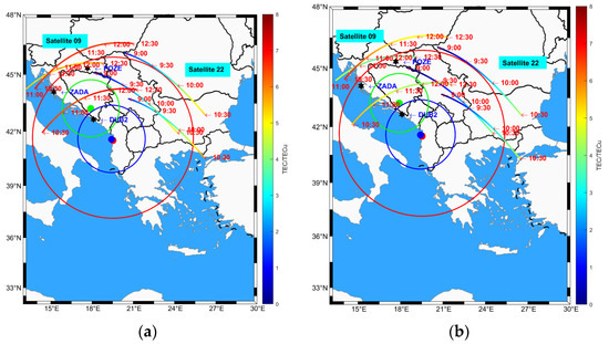
Figure 6.
POZE, ZADA and TUB2 station observed the IPP position and VTEC changes of satellite 09 and satellite 22 at UT 9:00–12:30. The left panels present TEC disturbance (TEC) along the IPP trajectories (trajectories are from left to right) in the vicinity of the epicenter on the previous day on November 25 (a) and the right panels show the day of the event on November 26 (b).
4.4. Observed Coseismic Ionospheric Disturbances in the Balkan Peninsula Seismic Swarm
To further analyze the CID, we examined TEC data with elevation angles higher than 20°. The TEC disturbance (dTEC) was obtained by employing high pass filtering.
In Figure 7, we compare the IPP trajectories and dTEC of satellite 16, 10, and 09 observed at the GPS stations. Abnormalities can be seen in the dTEC after the onset of the mainshock (26 November 2019) on earthquake day, but no such anomaly can be noted on the previous day or on the day after, respectively. In addition, it can be clearly seen that the anomaly of satellite 16 on the mainshock day is relatively weak, and the anomalies of satellite 10 and satellite 09 are more intense on the mainshock day. The IPPs of satellites 10 and 09 are approaching the source center. After three earthquakes in this area (25 November 2019), we noticed that the variation in the dtec amplitude of satellite 09 was about 0.15 tecu. Therefore, from this spatiotemporal analysis, we concluded that the intensified TEC disturbances in Figure 7 were likely of seismic origin.
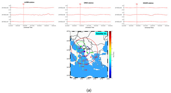
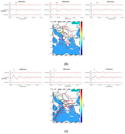
Figure 7.
The upper panels present TEC disturbance (dTEC) was observed on three consecutive days (25–27 November 2019, event day on 26 November 2019). The lower panels show their corresponding IPP trajectory of the satellite. (a) TEC disturbance (dTEC) on the previous day on 25 November 2019, on the event day on 26 November 2019, and on the day after on 25 November 2019, and the IPP trajectories of the GPS Sat. 16. (b) TEC disturbance (dTEC) on the previous day on 25 November 2019, on the event day on 26 November 2019, and on the day after on 25 November 2019, and the IPP trajectories of the GPS Sat. 10. (c) TEC disturbance (dTEC) on the previous day on 25 November 2019, on the event day on 26 November 2019, and on the day after on 25 November 2019, and the IPP trajectories of the GPS Sat. 09.
5. Discussions
In this paper, the PEIAs associated with a seismic swarm in Balkan Peninsula were studied. The TEC from ROB-TEC within the seismogenic zone showed significant enhancement before the mainshock day. Ionospheric anomalies caused by solar activity and geomagnetic activity can be excluded, suggesting that earthquakes were the factor in ionospheric anomalies. Temporal TEC from ROB-TEC showed profound variations during the 3–10 days before the mainshock on relatively quiet storm days (Figure 4). Such evidence has already been provided by multiple analyses of temporal TEC over epicentral regions. They (Ulukavak (2020); Nico (2021); Nina (2020)) analyzed global earthquakes with Mw ≥ 6 and possible ionospheric TEC anomalies that occurred before earthquakes. The results of this study contribute to earthquake prediction in the short-term by providing empirical evidence [33,34,35]. Biagi revealed the INFREP Radio Network variations in connection with six earthquakes (Mw > 5.0) that occurred in the Balkan Peninsula and Adriatic Sea on 26 and 27 November 2019 [36]. All this information increases our knowledge about the origin of different pre-seismic signals associated with the above-mentioned catastrophic earthquakes.
In addition, with the increase in the number of seismogenic zones, the incidence and intensity of ionospheric disturbance has increased, further analyses are needed to quantify the variations with a more statistical and mathematical model and method to convincingly prove such phenomena. However, there are many theories regarding the existence of abnormal TEC from GPS measurements and some have provided enough evidence for the connection of the lithosphere–atmosphere–ionosphere coupling system. For example, Freund has proved the existence of stress-activated electric currents in rocks that sweep through the mineral grains under stress dislocations and cause the peroxy links to break, thus generating flow-down stress gradients, constituting an electric current with attendant magnetic field variations and EM emissions. Further experiments have shown the generation of energetic charge barriers and their thermal conduction as fissure reactions in the seismogenic zone, which could be an intrinsic source of earthquake–ionospheric anomalies [37]. The main findings show that continuous earthquakes have repeatedly triggered the generation of high-energy charge barriers in the seismogenic belt and their heat conduction as crack reactions, which frequently affect the ionosphere.
On the other hand, CID observed by GPS stations (Figure 7) shows that with the increase in the number of earthquakes, the ionosphere over the seismogenic area is more obviously disturbed, which is consistent with the previous findings. For example, the far-field CID following the 2015 Mw 7.8 Nepal earthquake was detected by GPS-TEC [38] as the acoustic gravity wave induced by Rayleigh surface wave propagated into the ionosphere and caused the electronic and plasma density oscillation.
It is worth noting that after three strong earthquakes, the TEC suddenly decreased over the seismogenic area, forming a phenomenon similar to an ionospheric hole (Figure 6b). In further studies, more statistical and mathematical models and methods are required to prove such phenomena. There is evidence of a quantitative relationship between the TEC depression rate of the ionospheric cavity caused by the tsunami earthquake and the intensity of the tsunami earthquake [32,39]. However, more relevant observation data are needed to analyze the ionosphere at different heights in the region and the relevant meteorological data in the region are necessary for the generation of the ionospheric hole. In conclusion, the abovementioned results provide an opportunity to study the correlation between the ionosphere and earthquakes from multiple directions and angles for the earlier detection of specific pre-seismic anomalies related to earthquakes.
6. Conclusions
In this study, we presented research on pre-seismic ionospheric anomalies and CID for a seismic swarm in the Balkan Peninsula in November 2019. The results show that a larger number of positive anomalies appeared in the seismogenic area on 23 November 2019 (3 days before the earthquake), and continuous positive anomaly disturbances appeared in the grid points in the spatially overlapping seismogenic zones. Moreover, there was a small range of negative anomalies in the seismogenic area 6–12 days before the earthquake, although the interval was relatively long. We found that CID could be clearly observed at the stations in the seismogenic area during each earthquake, and the degree of CID and disturbance increased as the IPPs approached the center of the earthquake area. After the three earthquakes, we also found a similar ionospheric hole phenomenon over the seismogenic area, and a large area where the VTEC value plummeted over the seismogenic area. The results showed that with the increase in the number of seismogenic zones, the incidence and intensity of the ionospheric disturbance increased.
These findings suggest that there is synergy between different surface, atmospheric, and ionospheric processes. However, further analysis is required to support the hypothesis regarding lithosphere and ionosphere coupling during the earthquake preparation period as mainshock responses, which will be left for a future work.
Author Contributions
Conceptualization, J.L. and L.L.; methodology, L.W. and J.L.; validation, C.R., L.H. (Liangke Huang) and X.T.; formal analysis, L.W.; writing—original draft preparation, L.W., L.Z. and D.Z.; writing—review and editing, D.Z., J.L., L.H. (Ling Huang) and H.H.; funding acquisition, J.L., D.Z., L.H. (Ling Huang) and L.L. All authors have read and agreed to the published version of the manuscript.
Funding
This work was supported by the Guangxi Natural Science Foundation of China (2020GXNSFBA297145, 2020GXNSFBA159033), the Foundation of Guilin University of Technology (GUTQDJJ6616032), and the National Natural Science Foundation of China (42004025, 42064002).
Data Availability Statement
The data presented in this study are available on request from the corresponding author.
Conflicts of Interest
The authors declare no conflict of interest.
References
- Ikuta, R.; Hisada, T.; Karakama, G.; Kuwano, O. Stochastic Evaluation of Pre-Earthquake TEC Enhancements. J. Geophys. Res. Space Phys. 2020, 125, e2020JA027899. [Google Scholar] [CrossRef]
- Thomas, J.N.; Huard, J.; Masci, F. A statistical study of global ionospheric map total electron content changes prior to occurrences of M ≥ 6.0 earthquakes during 2000–2014. J. Geophys. Res. Space Phys. 2017, 122, 2151–2161. [Google Scholar] [CrossRef]
- Kakinami, Y.; Saito, H.; Yamamoto, T.; Chen, C.-H.; Yamamoto, M.-Y.; Nakajima, K.; Liu, J.-Y.; Watanabe, S. Onset Altitudes of Co-Seismic Ionospheric Disturbances Determined by Multiple Distributions of GNSS TEC after the Foreshock of the 2011 Tohoku Earthquake on March 9, 2011. Earth Space Sci. 2021, 8, e2020EA001217. [Google Scholar] [CrossRef]
- Davies, K.; Baker, D.M. Ionospheric effects observed around the time of the Alaskan earthquake of March 28, 1964. J. Geophys. Res. (1896–1977) 1965, 70, 2251–2253. [Google Scholar] [CrossRef]
- Pulinets, S. Ionospheric precursors of earthquakes; recent advances in theory and practical applications. Terr. Atmos. Ocean. Sci. 2004, 15, 413–436. [Google Scholar] [CrossRef]
- Sanchez, S.A.; Kherani, E.A.; Astafyeva, E.; de Paula, E.R. Ionospheric Disturbances Observed Following the Ridgecrest Earthquake of 4 July 2019 in California, USA. Remote Sens. 2022, 14, 188. [Google Scholar] [CrossRef]
- Liu, J.; Chen, Y.; Chuo, Y.; Tsai, H. Variations of ionospheric total electron content during the Chi-Chi earthquake. Geophys. Res. Lett. 2001, 28, 1383–1386. [Google Scholar] [CrossRef]
- Chen, Y.-I.; Liu, J.-Y.; Tsai, Y.-B.; Chen, C.-S. Statistical tests for pre-earthquake ionospheric anomaly. Terr. Atmos. Ocean. Sci. 2004, 15, 385–396. [Google Scholar] [CrossRef]
- Hobara, Y.; Parrot, M. Ionospheric perturbations linked to a very powerful seismic event. J. Atmos. Sol.-Terr. Phys. 2005, 67, 677–685. [Google Scholar] [CrossRef]
- Ryu, K.; Lee, E.; Chae, J.; Parrot, M.; Pulinets, S. Seismo-ionospheric coupling appearing as equatorial electron density enhancements observed via DEMETER electron density measurements. J. Geophys. Res. Space Phys. 2014, 119, 8524–8542. [Google Scholar] [CrossRef]
- Chen, P.; Yao, Y.; Yao, W. On the coseismic ionospheric disturbances after the Nepal Mw7. 8 earthquake on April 25, 2015 using GNSS observations. Adv. Space Res. 2017, 59, 103–113. [Google Scholar] [CrossRef]
- Shah, M.; Aibar, A.C.; Tariq, M.A.; Ahmed, J.; Ahmed, A. Possible ionosphere and atmosphere precursory analysis related to Mw> 6.0 earthquakes in Japan. Remote Sens. Environ. 2020, 239, 111620. [Google Scholar] [CrossRef]
- Fernández, J. Geodetic and geophysical effects associated with seismic and volcanic hazards. In Geodetic and Geophysical Effects Associated with Seismic and Volcanic Hazards; Springer: Berlin/Heidelberg, Germany, 2004; pp. 1301–1303. [Google Scholar]
- Liu, J.-Y.; Chen, Y.; Chuo, Y.; Chen, C.-S. A statistical investigation of preearthquake ionospheric anomaly. J. Geophys. Res. Space Phys. 2006, 111, A5. [Google Scholar] [CrossRef]
- Kumar, S.; Chen, W.; Liu, Z.; Ji, S. Effects of solar and geomagnetic activity on the occurrence of equatorial plasma bubbles over Hong Kong. J. Geophys. Res. Space Phys. 2016, 121, 9164–9178. [Google Scholar] [CrossRef]
- Zheng, D.; Zheng, H.; Wang, Y.; Nie, W.; Li, C.; Ao, M.; Hu, W.; Zhou, W. Variable pixel size ionospheric tomography. Adv. Space Res. 2017, 59, 2969–2986. [Google Scholar] [CrossRef]
- Dobrovolsky, I.; Zubkov, S.; Miachkin, V. Estimation of the size of earthquake preparation zones. Pure Appl. Geophys. 1979, 117, 1025–1044. [Google Scholar] [CrossRef]
- Bergeot, N.; Chevalier, J.-M.; Bruyninx, C.; Pottiaux, E.; Aerts, W.; Baire, Q.; Legrand, J.; Defraigne, P.; Huang, W. Near real-time ionospheric monitoring over Europe at the Royal Observatory of Belgium using GNSS data. J. Space Weather. Space Clim. 2014, 4, A31. [Google Scholar] [CrossRef]
- Liu, J.Y.; Chuo, Y.; Shan, S.; Tsai, Y.; Chen, Y.; Pulinets, S.; Yu, S. Pre-earthquake ionospheric anomalies registered by continuous GPS TEC measurements. In Annales Geophysicae; Copernicus GmbH: Göttingen, Germany, 2004; pp. 1585–1593. [Google Scholar]
- Liu, J.-Y.; Chen, Y.; Chen, C.-H.; Liu, C.; Chen, C.; Nishihashi, M.; Li, J.; Xia, Y.; Oyama, K.; Hattori, K. Seismoionospheric GPS total electron content anomalies observed before the 12 May 2008 Mw7. 9 Wenchuan earthquake. J. Geophys. Res. Space Phys. 2009, 114. [Google Scholar] [CrossRef]
- Cahyadi, M.N.; Heki, K. Ionospheric disturbances of the 2007 Bengkulu and the 2005 Nias earthquakes, Sumatra, observed with a regional GPS network. J. Geophys. Res. Space Phys. 2013, 118, 1777–1787. [Google Scholar] [CrossRef]
- Dong, Y.; Gao, C.; Long, F.; Yan, Y. Suspected Seismo-Ionospheric Anomalies before Three Major Earthquakes Detected by GIMs and GPS TEC of Permanent Stations. Remote Sens. 2022, 14, 20. [Google Scholar] [CrossRef]
- Zheng, D.; Yao, Y.; Nie, W.; Chu, N.; Lin, D.; Ao, M. A new three-dimensional computerized ionospheric tomography model based on a neural network. GPS Solut. 2020, 25, 10. [Google Scholar] [CrossRef]
- Zheng, D.; Yao, Y.; Nie, W.; Liao, M.; Liang, J.; Ao, M. Ordered subsets-constrained ART algorithm for ionospheric tomography by combining VTEC data. IEEE Trans. Geosci. Remote Sens. 2020, 59, 7051–7061. [Google Scholar] [CrossRef]
- Rao, P.; Ram, S.T.; Krishua, S.; Niranjan, K.; Prasad, D. Morphological Characteristics of L-Band Scintillations and Their Impact on GPS Signals—A Quantitative Study on the Precursors for the Occurrence of Scintillations; Andhra University Vishakhapatnam (India) Deptartment of Physics: Visakhapatnam, India, 2006. [Google Scholar]
- Filjar, R.; Kos, S.; Krajnovic, S. Dst Index as a Potential Indicator of Approaching GNSS Performance Deterioration. J. Navig. 2013, 66, 149–160. [Google Scholar] [CrossRef]
- Jin, S.; Occhipinti, G.; Jin, R. GNSS ionospheric seismology: Recent observation evidences and characteristics. Earth-Sci. Rev. 2015, 147, 54–64. [Google Scholar] [CrossRef]
- Heki, K.; Enomoto, Y. Preseismic ionospheric electron enhancements revisited. J. Geophys. Res. Space Phys. 2013, 118, 6618–6626. [Google Scholar] [CrossRef]
- Rolland, L.M.; Lognonné, P.; Astafyeva, E.; Kherani, E.A.; Kobayashi, N.; Mann, M.; Munekane, H. The resonant response of the ionosphere imaged after the 2011 off the Pacific coast of Tohoku Earthquake. Earth Planets Space 2011, 63, 853–857. [Google Scholar] [CrossRef]
- Astafyeva, E.; Shalimov, S.; Olshanskaya, E.; Lognonné, P. Ionospheric response to earthquakes of different magnitudes: Larger quakes perturb the ionosphere stronger and longer. Geophys. Res. Lett. 2013, 40, 1675–1681. [Google Scholar] [CrossRef]
- Occhipinti, G.; Kherani, E.A.; Lognonné, P. Geomagnetic dependence of ionospheric disturbances induced by tsunamigenic internal gravity waves. Geophys. J. Int. 2008, 173, 753–765. [Google Scholar] [CrossRef]
- Kakinami, Y.; Kamogawa, M.; Tanioka, Y.; Watanabe, S.; Gusman, A.R.; Liu, J.Y.; Watanabe, Y.; Mogi, T. Tsunamigenic ionospheric hole. Geophys. Res. Lett. 2012, 39. [Google Scholar] [CrossRef]
- Ulukavak, M.; Yalçınkaya, M.; Kayıkçı, E.T.; Öztürk, S.; Kandemir, R.; Karslı, H. Analysis of ionospheric TEC anomalies for global earthquakes during 2000–2019 with respect to earthquake magnitude (Mw ≥ 6.0). J. Geodyn. 2020, 135, 101721. [Google Scholar] [CrossRef]
- Nico, G.; Biagi, P.F.; Ermini, A.; Boudjada, M.Y.; Eichelberger, H.U.; Katzis, K.; Contadakis, M.; Skeberis, C.; Moldovan, I.A.; Bezzeghoud, M. Wavelet analysis applied on temporal data sets in order to reveal possible pre-seismic radio anomalies and comparison with the trend of the raw data. In EGU General Assembly 2021; Copernicus GmbH: Göttingen, Germany, 2021. [Google Scholar]
- Nina, A.; Pulinets, S.; Biagi, P.F.; Nico, G.; Mitrović, S.T.; Radovanović, M.; Popović, L.C. Variation in natural short-period ionospheric noise, and acoustic and gravity waves revealed by the amplitude analysis of a VLF radio signal on the occasion of the Kraljevo earthquake (Mw = 5.4). Sci. Total Environ. 2020, 710, 136406. [Google Scholar] [CrossRef]
- Ulukavak, M.; Yalcinkaya, M. Precursor analysis of ionospheric GPS-TEC variations before the 2010 M 7.2 Baja California earthquake. Geomat. Nat. Hazards Risk 2017, 8, 295–308. [Google Scholar] [CrossRef]
- Freund, F. Toward a unified solid state theory for pre-earthquake signals. Acta Geophys. 2010, 58, 719–766. [Google Scholar] [CrossRef]
- Liu, H.; Zhang, K.; Imtiaz, N.; Song, Q.; Zhang, Y. Relating Far-Field Coseismic Ionospheric Disturbances to Geological Structures. J. Geophys. Res. Space Phys. 2021, 126, e2021JA029209. [Google Scholar] [CrossRef]
- Savastano, G.; Komjathy, A.; Shume, E.; Vergados, P.; Ravanelli, M.; Verkhoglyadova, O.; Meng, X.; Crespi, M. Advantages of geostationary satellites for ionospheric anomaly studies: Ionospheric plasma depletion following a rocket launch. Remote Sens. 2019, 11, 1734. [Google Scholar] [CrossRef]
Publisher’s Note: MDPI stays neutral with regard to jurisdictional claims in published maps and institutional affiliations. |
© 2022 by the authors. Licensee MDPI, Basel, Switzerland. This article is an open access article distributed under the terms and conditions of the Creative Commons Attribution (CC BY) license (https://creativecommons.org/licenses/by/4.0/).