Article

Mixed Feature Prediction on Boundary Learning for Point Cloud Semantic Segmentation

The State Key Laboratory of Integrate Service Network, School of Telecommunications Engineering, Xidian University, Xi’an 710071, China
*
Author to whom correspondence should be addressed.
Remote Sens. 2022, 14(19), 4757; https://doi.org/10.3390/rs14194757
Submission received: 28 July 2022 / Revised: 30 August 2022 / Accepted: 15 September 2022 / Published: 23 September 2022

Abstract

:
Existing point cloud semantic segmentation approaches do not perform well on details, especially for the boundary regions. However, supervised-learning-based methods depend on costly artificial annotations for performance improvement. In this paper, we bridge this gap by designing a self-supervised pretext task applicable to point clouds. Our main innovation lies in the mixed feature prediction strategy during the pretraining stage, which facilitates point cloud feature learning with boundary-aware foundations. Meanwhile, a dynamic feature aggregation module is proposed to regulate the range of receptive field according to the neighboring pattern of each point. In this way, more spatial details are preserved for discriminative high-level representations. Extensive experiments across several point cloud segmentation datasets verify the superiority of our proposed method, including ShapeNet-part, ScanNet v2, and S3DIS. Furthermore, transfer learning on point cloud classification and object detection tasks demonstrates the generalization ability of our method.

Graphical Abstract

1. Introduction

With the remarkable advancements in computer vision, artificial intelligence, and sensor technology, 3D vision has received considerable crucial attention. Semantic segmentation based on point clouds has been widely adopted in the fields of remote sensing [1,2], autonomous driving [3,4], smart city [5], agricultural resource assessment [6], etc. However, existing methods can not segment well on details such as at point cloud boundaries, which has a serious impact on the practical application. Recently, a new paradigm named transformer has provided a powerful ability for feature learning with a superior structure. Nevertheless, the performance enhancement for supervised-learning-based methods depends on costly manual labeling of datasets with high precision. Furthermore, the generalization ability of such methods for different applications remains a big challenge.
Recent progress in deep learning has extended the self-supervised pretraining technology to language and image processing tasks [7,8]. By designing an auxiliary pretext task, models are often pretrained first to obtain representations that are more suitable for downstream tasks. The mask and predict (MAP) strategy has been phenomenally successful in pretraining tasks [9,10,11,12]. Nevertheless, most of these approaches rely on reconstruction [13,14,15] or generation works [16], which are challenging for point cloud data due to their unordered nature. Furthermore, another fatal issue in point cloud analysis is feature aggregation. Since not every member shares the same weight in the local region, adopting kernels with rigid sizes for point feature aggregation is inherently limited.
In this paper, we propose a novel framework to address the aforementioned challenges from three aspects. First, we design a pretext task aiming at delivering a boundary-aware model for point cloud semantic segmentation. Through a high-pass filter for point clouds, the pretraining task attempts to regress the target sharp features of point clouds by mixing the boundary features. As shown in Figure 1, we first locate the boundary points and then swap the features with their farthest local neighbors. Therefore, by using mixed boundaries to predict sharp features, we encourage the model to be boundary-aware in the pretraining stage. Second, we develop a dynamic feature aggregation (DFA) module to select discriminative neighbors with the consideration of spatial information. This module helps to raise the proportion of detailed information fed into the pooling module. Consequently, the latent representation is spatially more precise. Third, a boundary-label consistent loss is introduced to evaluate the predicted boundaries based on the segmentation results, which is jointly optimized with the cross-entropy loss. Experimental verifications of our proposed model are performed on different semantic segmentation datasets. After comparison, our method produces more accurate results in the boundary regions. Furthermore, we transfer our network to the point cloud classification (on the ModelNet40 and ScanObjectNN datasets) and object detection task (on the SUNRGB-D dataset). The results demonstrate the applicability of our method to general 3D processing tasks.
To summarize, the major contributions of this work are presented as follows:
  • We design a mixed feature prediction task for point cloud semantic segmentation to pretrain the model to be boundary-aware.
  • A dynamic feature aggregation module is proposed to perform point convolutions with adaptive receptive fields, which introduces more spatial details to the high-level feature representations.
  • Experimental results validate the enhancement of our method for boundary regions in semantic segmentation predictions. In addition, the integrated feature representations learned by our method transfer well to other point cloud tasks such as classification and object detection.

2. Related Work

2.1. Point Cloud Semantic Segmentation Methods

Point cloud semantic segmentation is an indispensable critical step in point cloud processing. Its principle is to divide point cloud data into several nonintersecting subsets according to the characteristic properties of point clouds. Traditional point cloud segmentation methods include edge-based, region-based, and model-fitting based methods [17,18,19], only obtaining a relative coarse segmentation result. Recently, with the development of data-driven deep learning algorithms, end-to-end methods are proposed to analyze point clouds. As a pioneering work of learning-based method, PointNet [20] provided a network architecture that was suitable for processing raw point clouds directly. To further exploit local features, PointNet++ [21] sought out a solution by dividing the entirety at different scales. However, the aggregation manner for the global feature was still an intractable question. KPConv [22] employed irregular convolution operators to map pointwise features to predefined kernel points, and carried out convolution operations with regular kernel points. Recently, the transformer-based methods [23,24,25] possessing a large number of parameters were introduced to explore the long-range relations among points. In this work, we propose a self-supervised pretraining method on point clouds, providing an essential initialization for semantic segmentation tasks.

2.2. Self-Supervised Learning

Self-supervised pretraining has become increasingly popular due to its effectiveness in many research fields, such as natural language processing [7,8], target detection [26], pose estimation [27], and 3D reconstruction [28]. BERT [7] introduced a masked language modeling (MLM) strategy to mask and recover the input tokens. MAE [12] encoded incomplete patches with an autoencoder and reconstructed the original image through a lightweight decoder. Li et al. [29] used multiview relevance to generate supervision signals for training a 2D-to-3D pose estimator. Recently, several current works [24,30,31] advised to use self-supervised pretraining techniques for 3D point clouds. Sauder et al. [32] presented a pretraining method based on rearranging permuted point clouds. Compared to the jigsaw puzzles in images [33], Eckart et al. [30] designed a pretext task to partition the point clouds to interpret a latent Gaussian mixture model. Inspired by the BERT-style in NLP, Point-BERT [11] first converted point clouds to discrete tokens via dVAE, and then performed pretraining by predicting the masked point tokens. However, most of the existing pretraining tasks for point clouds are based on generative or contrastive methods. It is inconducive for downstream tasks, such as semantic segmentation, which require more geometric features to reflect local information.

2.3. Boundary Learning in Segmentation

In 2D image processing, the problems of blurred target boundaries and inaccurate predictions in segmentation tasks can be effectively improved by jointly executing boundary detection and semantic segmentation. Li et al. [34] decoupled edge and body areas by extracting the high-frequency components and low-frequency components of the image. Distinct optimizations were performed on different parts of the pixels. Zhen et al. [35] designed a pyramid context module that shared semantic information for joint task learning, refining details along object boundaries. However, it remained a tough problem for point clouds to incorporate boundary features with the point branches. EC-Net [36] detected point cloud boundaries by a deep architecture and accomplished a fine-grained 3D reconstruction with sharp features reserved. Jiang et al. [37] constructed a hierarchical graph to embed edge features with the point features progressively. JSENet [38] proposed a two-stream fully convolutional network to settle the edge detection problem and the segmentation problem at the same time. CBL [31] explored the boundary areas with contrastive learning and enhanced performance on different baselines. However, due to the sparse distribution and variable scales, the boundary features remained difficult to capture adequately.

3. Methods

3.1. Overview

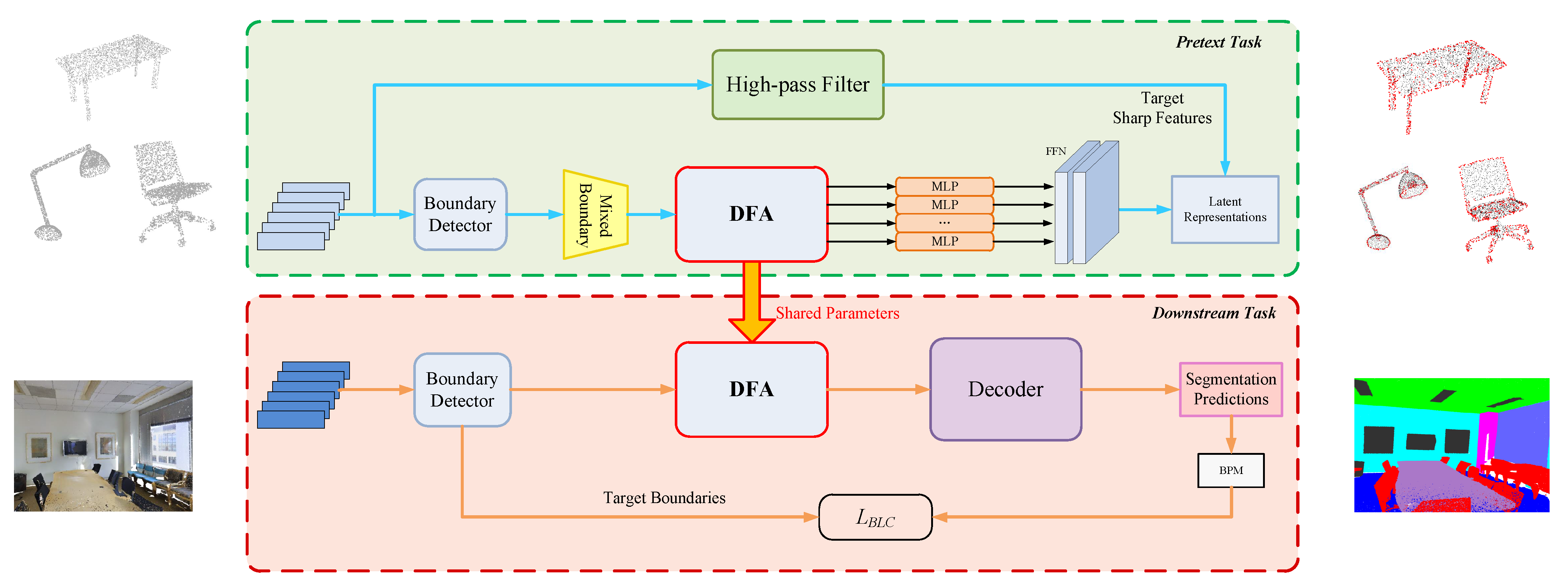
In this section, we present the overall framework of our model on boundary learning for the point cloud semantic segmentation task. Given point clouds denoted as P R N × 3 , we first detected boundaries and mixed the features between the boundary points and the interior points. With this boundary-blurred outcome fed into the model, we directly regressed the sharp features of the point clouds. After this self-supervised pretext task, the pretrained model was applied to the downstream task, fine-tuned with task-specific decoders. In particular, to better preserve detailed information in high-level feature propagation, we adopted dilated grouping and hybrid feature encoding strategies. In addition, a global label-consistent loss was introduced to ensure the segmentation correctness around boundary regions. Figure 2 illustrates the detailed pipeline of our boundary-aware model.

3.2. Masked Feature Pretraining

3.2.1. Boundary Detector

The boundary regions of point clouds share a distinct spatial distribution characteristic that most neighbor points locate only in some directions. For a query point P i in point clouds, we first sought its nearest neighbors as N i = p j | j = 1 , 2 , k through a k-dimensional (k-d) tree. Considering the density of each local region, we then computed the coordinate value of the shape center with the following equation:
C i = 1 k j = 1 k S ( x j , y j , z j ) p j S ( x i , y i , z i )
where k is the number of local neighbors, S ( x , y , z ) is an inverse density function provided by kernel density estimation, and p j is the spatial coordinates of local neighbors. By calculating the L 2 distance between the shape center and the centroid point, we could identify the marginal regions. Considering the density variation of local regions, the resolution r N i was defined as the minimum distance between a centroid point and its neighbor point.
r N i = min p j N i P i p j 2
We set a threshold value λ to extract the boundary points in marginal regions, as defined in Equation (3):
C i P i > λ · r N i

3.2.2. Mixed Feature Prediction Task

Motivated by MAE [12] and Point-BERT [11], we wanted to extend this self-supervised method to point cloud segmentation. Nevertheless, it is challenging to extend this mask and model strategy to the unorganized point cloud data. Unlike the regular arrangement of two-dimensional images, the decoder for point clouds needs to recover the coordinate position of the masked points. Moreover, there is no well-defined local partition manner to build a shape vocabulary for point clouds. Point-BERT [11] adds an external tokenizer for the pretraining task, but extra training is required for the tokenizer in the workflow. Another common solution to obtain local embeddings for point clouds is to utilize the basic sampling and grouping operations. Nevertheless, the process of sampling introduces randomness to the same input, which increases the difficulty to reconstruct the masked point clouds for the decoder.
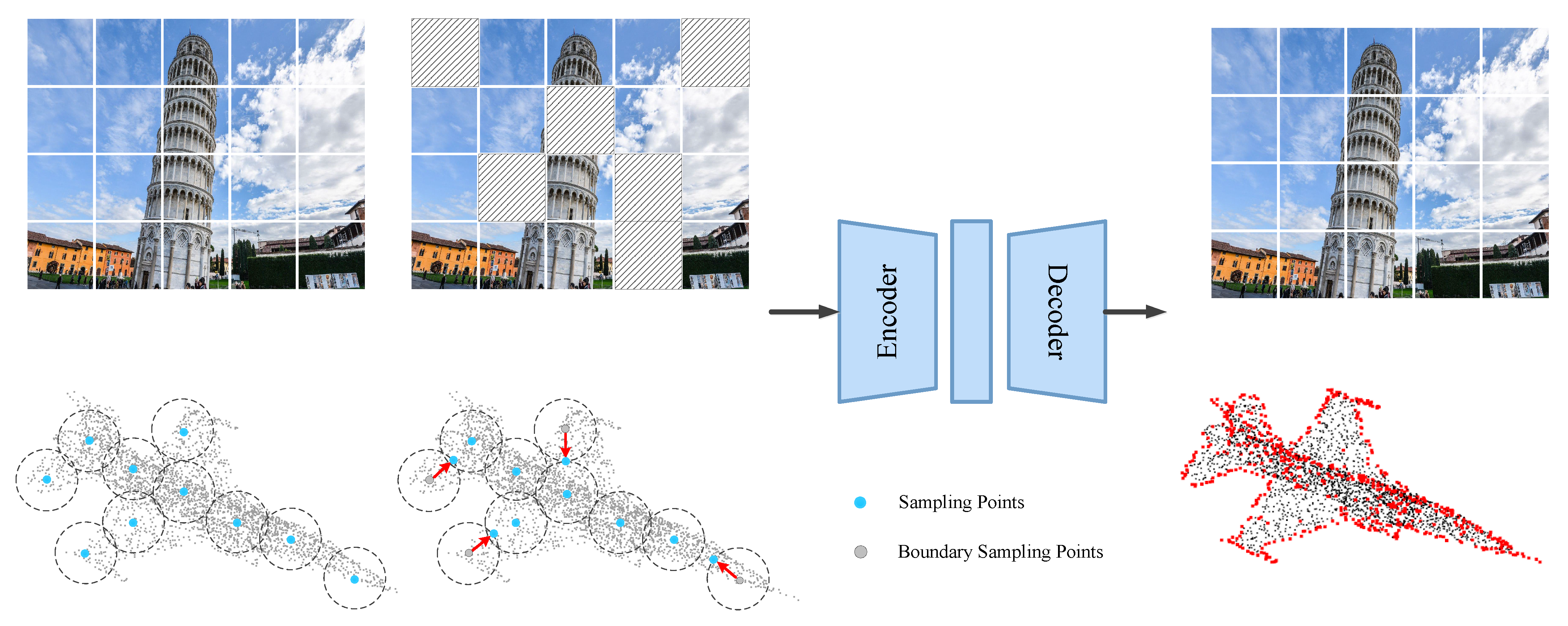
To solve the problems above, we adopted a mix and predict strategy as in Figure 3 to generate a pretext task for pretraining. Specifically, we first utilized a boundary detector to extract and mask boundary points. Then, we found its K surrounding neighbors for each point, forming a continuous local region. Inspired by the PointCutMix [39] technique, we randomly selected the sampling points and swapped its features with those of its farthest local neighbor. Finally, a boundary-mixed coarse input was fed into the encoder module. As for the decoder, we selected the sharp features of point clouds as the target prediction. In this way, the encoder was encouraged to capture the sharp features from the coarse input formed by inner points. Moreover, for the same set of point cloud targets, the sharp edge features were explicit regardless of the variability of the sampling results. The spatial coordinate information was also reserved, and no additional learning was required for the decoder.
The goal of our mixed feature prediction task was to boost the ability of our model to recognize boundaries. Through a high-pass filter, we could obtain the sharp features of the point clouds. The geometric information could be directly served as a continuous supervision signal to pretrain our model. After the feature aggregation through a MLP, we computed the L 2 distance between the predicted sharp features and the original sharp features as in Equation (4). The pretext task performed self-supervised learning by locating boundaries, which was helpful to improve the training of the model with limited data.
L o s s p r e = i = 1 N F s _ p r e d F s _ t g t 2
where N represents the point number and F s _ p r e d and F s _ t g t represent the predicted sharp features and the original target sharp features, respectively.

3.2.3. High-Pass Filter

The sharp features describe the contour area and the corner sets of point clouds, reflecting the local structural information that entails semantic meaning. In this paper, we regarded the point clouds as an undirected graph signal G = ( V , A ) , where V represents the set of the nodes and A represents the relationship between nodes. The relations between two nodes were defined as:
A i j = σ T x i x j 2
where x i and x j are the feature vectors of node i and node j. · 2 represents the L 2 norm distance, T is a nonlinear function which we implemented as a shared multilayer perceptron (MLP), and σ is the activation function; we adopted a LeakyRelu in the practical experiment. Hence, A = a i , j R N × N is the adjacent matrix of graph G. In this way, we could resort to the spectral graph theory to analyze disordered point clouds. The Laplace matrix of the graph G was obtained as follows:
L = D A
where D is a diagonal matrix consisting of the degrees of each node in G. To eliminate the influence of scale variation, we normalized the Laplace matrix as follows:
L ^ = I D 1 2 A D 1 2
After an eigendecomposition as in Equation (8), the eigenvalues represented different frequency components of the graph signal.
L ^ = U Λ U 1 = U λ 1 λ n U 1
where Λ represents the frequency response of the point clouds. In general, the eigenvalues are sorted in a descending order as λ 1 λ 2 λ n . By designing an attention mechanism, we could update the node aggregations by focusing on high-frequency information to generate the sharp features. Practically, we used the Haar-like filter [40] h ( Λ ) , which is a special case of the Chebyshev polynomial approximation of GCN. As shown in Equation (9), the frequency response of h ( Λ ) was 1 λ i . Due to the condition that 1 λ i 1 λ i + 1 , the signal passing through this filter was amplified in the high-frequency regions and suppressed in the low-frequency regions, achieving the effect of a high-pass filter as below:
h ( Λ ) = I L ^
In Figure 4, the target sharp features of the input point clouds P for the pretraining task was obtained as h Λ P . Actually, the sharp features reflect the change variation of each node to its neighbors.

3.3. Dynamic Feature Aggregation

For most point cloud processing baselines, high-level features contain limited spatial information due to the inevitable pooling operations. To preserve more spatial details, one straightforward solution is to collect more spatial information before pooling. So in this work, we first clustered the point clouds with boundary-based location information for separately encoding. Then, we adopted three grouping strategies with different dilated ratios to perform feature aggregation. Finally, the boundary regions containing the most detailed information fused hybrid grouping results with the most kinds of dilated ratios.

3.3.1. Spatial-Based Clustering

Points located in different position of the point cloud have different importance. Therefore, it is inefficient to perform the same calculation for each point. To adequately exploit the feature relations between local regions, we divided the input feature map into three branches based on the boundary detector in Section 3.2.1, denoted as boundary regions, cross regions, and interior regions. After extracting the boundary points, we counted the number of boundary points in each local region. The cluster criterion is given as follows:
P i interior regions , b i = 0 cross regions , 0 < b i < μ boundary regions , μ < b i
where μ is a threshold parameter. b i denotes the number of boundary points surrounding the point P i . The threshold parameter μ is determined by calculating the 3D chamfer distance between the points from boundary cluster and the points from boundary detector as follows,
d CD P , Q = 1 N p p P min q Q p q 2 2 + 1 N q q Q min p P q p 2 2
where P and Q represent the points from the boundary cluster and the points extracted by the boundary detector, respectively. N p and N q represent the number of point sets P and Q.

3.3.2. Hybrid Feature Encoder

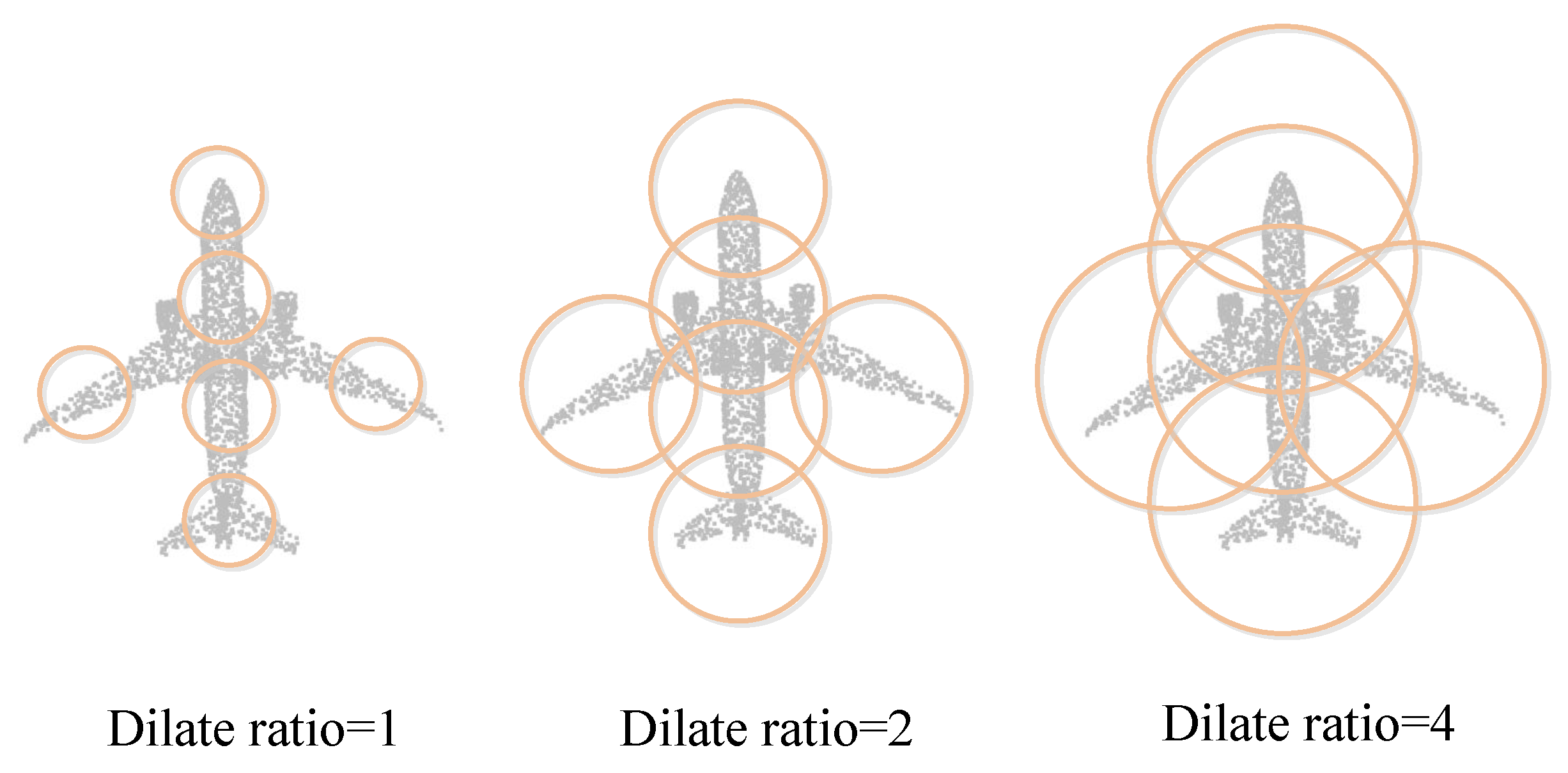
Searching K nearest neighbors is a commonly used grouping method for each sampling point. However, merely using a rigid selection criterion can not suitably reflect the geometric and structural properties of point clouds, which is redundant or even inefficient, especially dealing with flat regions. To solve this problem, we put forward a dilated neighbor selection strategy for point grouping. As shown in Figure 5, a wider range of points was considered by applying our predefined n dilated searching rates. In this process, we obtained K nearest neighbors for each dilated ratio. As the dilated ratio increased, the neighborhood range of each point increased accordingly.
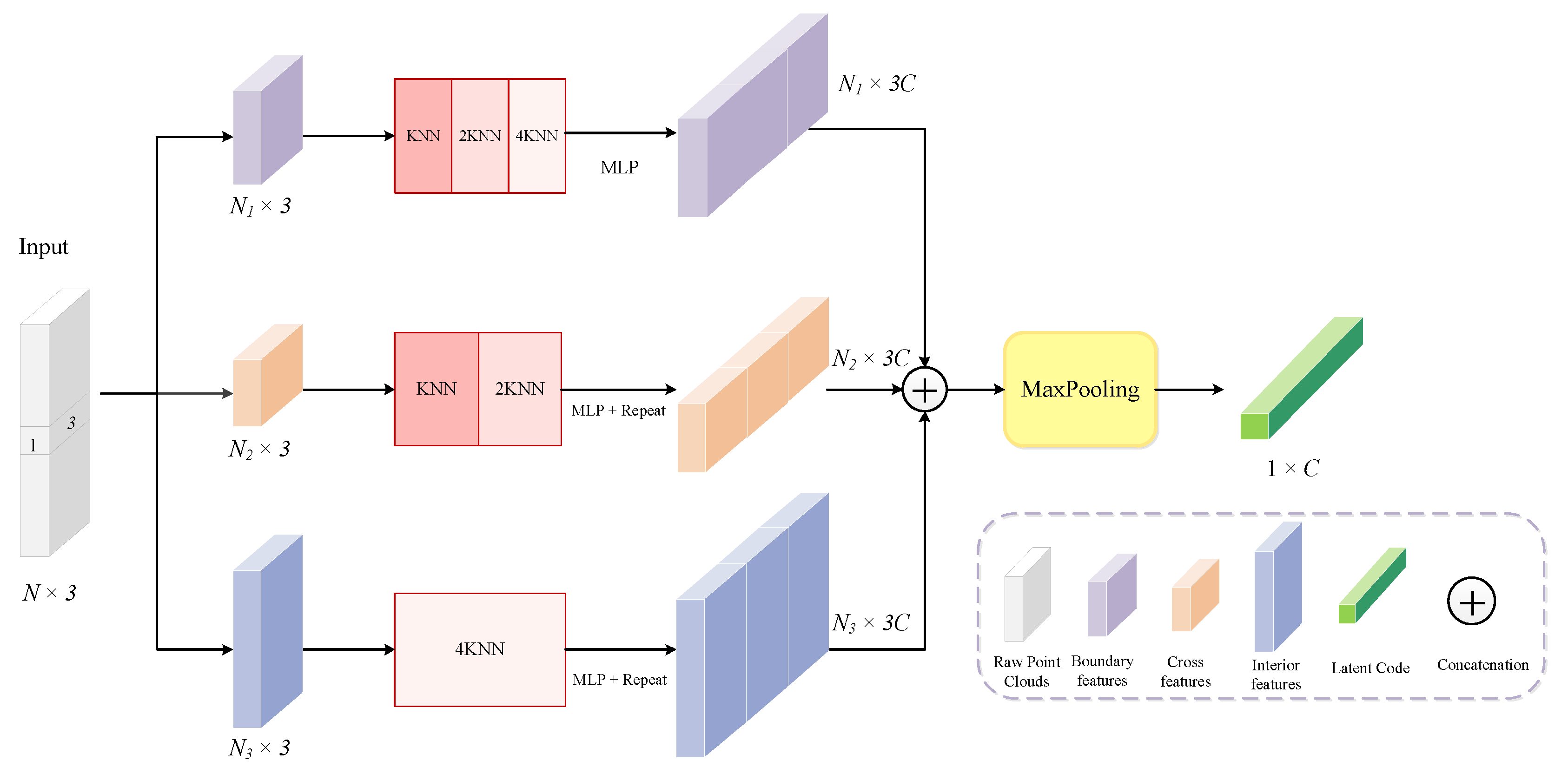
To ensure the symmetric invariance of the point cloud processing network, pooling modules are necessary for point feature encoders. Unfortunately, such an operation results in the loss of spatial information, which is harmful to pointwise prediction for segmentation. To alleviate this issue, we enriched the components of boundary region features before pooling. The overall structure of our proposed DFA module is shown in Figure 6. The module consisted of three branches corresponding to the boundary, cross, and interior regions, respectively. According to the various feature distribution of different regions, we adopted three kinds of dilated ratios for a reasonable neighbor grouping. In particular, we stacked all of the neighbor points with the dilated ratios of 1, 2, 4 for the boundary regions, neighbor points with the dilated ratios of 1 and 2 for the cross regions, and the dilated ratio of 4 for the interior regions. The use of dilated grouping can not only integrate multiscale information but also augment the diversity of spatial detail information. After employing an MLP to build feature maps F, we fed the outcomes to the max-pooling block and obtained a comprehensive latent representation.

3.4. Loss Function

To better explore boundary regions in the segmentation results, we constrained the final result with a label-consistent loss. Given the predicted category of each point, we obtained the boundary prediction result by analyzing the categories of its neighboring points. Specifically, for each point, we first counted the number of neighbors of each category within a certain range and then calculated the proportion of points different from the category of the point. If the proportion was greater than the preset ratio value, the point was identified as a boundary point; otherwise, it was not. As the boundary detector results could be regarded as the supervision information, we computed the chamfer distance of the label boundaries b i and the predicted boundaries b ^ j :
L B L C = i = 1 m j = 1 k b i b ^ j 2
Finally, we explored the boundary regions based on a global correction and the final loss was
L = L c r o s s e n t r o p y + θ L B L C
where θ is the loss weight.

4. Experiments

In this section, we introduce the implementation details for our approach. We first provide the setups of the pretraining scheme. Then, we evaluate the performance of our model on downstream tasks. The evaluation metrics and corresponding comparison results with other state-of-the-art works are shown in detail. Our network was implemented in Pytorch, with two parallel Nvidia GTX 2080Ti GPUs employed for training.

4.1. Experiment Setups

4.1.1. Pretraining Setups

ShapeNet [41] was selected for the pretraining of our network; it contains over 57,448 models with 55 categories. We split the datasets into a training set and a validation set. Each model was sampled for 1024 points. In the pretraining phase, we employed the AdamW [42] optimizer with an initial learning rate set to 0.001 and a weight decay of 0.3. The model was trained for 600 epochs and the batch size was set to 64. For the boundary point detector, the optimal results for Equation (3) was achieved at λ = 8 on the ShapeNet and the clustering threshold parameter μ in Equation (10) was 12 in our experiments.

4.1.2. Evaluation Metrics

We selected overall accuracy (OA), average accuracy (mAcc), and mean IoU (mIoU) as the evaluation metrics for the downstream tasks on point clouds. OA denotes overall accuracy, i.e., the proportion of the correct predicted points to the total number of points. mAcc denotes the mean value of the prediction accuracy for all categories. mIoU denotes the mean value of IoUs corresponding to different categories, where IoU denotes the ratio of the intersection and union of two sets of ground truths and predictions. The calculation formulas for the evaluation metrics are shown as follows,
O A = i = 1 N P i i i = 1 N j = 1 N P i j
m A c c = 1 N * i = 1 N P i i j = 1 N P i j
m I o U = i = 1 N I o U i N , I o U i = i = 1 N P i i j = 1 N P i j + j = 1 N P j i P i i
where N is the total number of the categories. P i j represents the number of points that belong to category i but are classified as category j. P i i represents the number of points correctly predicted in category i. P j i represents the number of points that belong to category j but are classified as category i.

4.2. Downstream Tasks

4.2.1. Part Segmentation on ShapeNet-Part Dataset

The ShapeNet-part dataset [43] is composed of 16,881 3D models covering 16 categories. Each category is divided into 2 to 6 parts, resulting in 50 parts in total. The dataset was split into training, validation, and testing set, containing 12137, 1870, and 2874 models, respectively. The dataset is practically challenging due to its imbalanced distribution of the model categories and parts within the category. The results of the proposed method and some current state-of-the-art methods on the ShapeNet-part dataset are presented in Table 1.

4.2.2. Semantic Segmentation on ScanNet v2 Dataset

ScanNet v2 [48] was built using 2.5 million scans from 1613 3D indoor scenes, with 21 semantic classes included. The dataset contains 3D coordinate information and label information in a mesh format. A train/validation/test split of 1201/312/100 is provided for the public. Following previous work [49], we randomly sampled 8192 points from each room for training and testing over the entire scene. In the training phase, we employed the AdamW [42] optimizer with an initial learning rate set to 0.001 and a weight decay of 0.3. The model was trained for 300 epochs and the batch size was set to 32.
As shown in Table 2, we compared the classwise mean of intersection over union (mIoU) of our method to some outstanding networks. Our network ranked third after Mix3D [42] and O-CNN [50]. Mix3D uses an out-of-context technique for data augmentation and reach the state-of-the-art scores based on a voxel-based method [51], which depends on costly computation complexity. O-CNN [50] is also a full-voxel-based solution that leverages an octree structure. Notably, our method outperformed other point-based methods by a large margin. JSENet [38] and CBL [31] are methods considering boundaries for point clouds; our method achieved a performance improvement of 5.9% and 5.3%, respectively, against these methods.

4.2.3. Semantic Segmentation on S3DIS Dataset

S3DIS [53] refers to the Large-Scale 3D Indoor Spaces dataset obtained by a Matterport scanner; it contains 271 rooms from six different areas. Each point in the scene is represented by a semantic label in 13 categories (chair, table, wall, etc.). We divided the rooms into 1 m × 1 m blocks and randomly sample 4096 points for each block. As the experimental setups used in [54], we selected Area 5 for testing and the other areas for training in default. In the training phase, we employed the AdamW [42] optimizer with an initial learning rate set to 0.0001 and a weight decay of 0.3. The model was trained for 300 epochs and the batch size was set to 32.
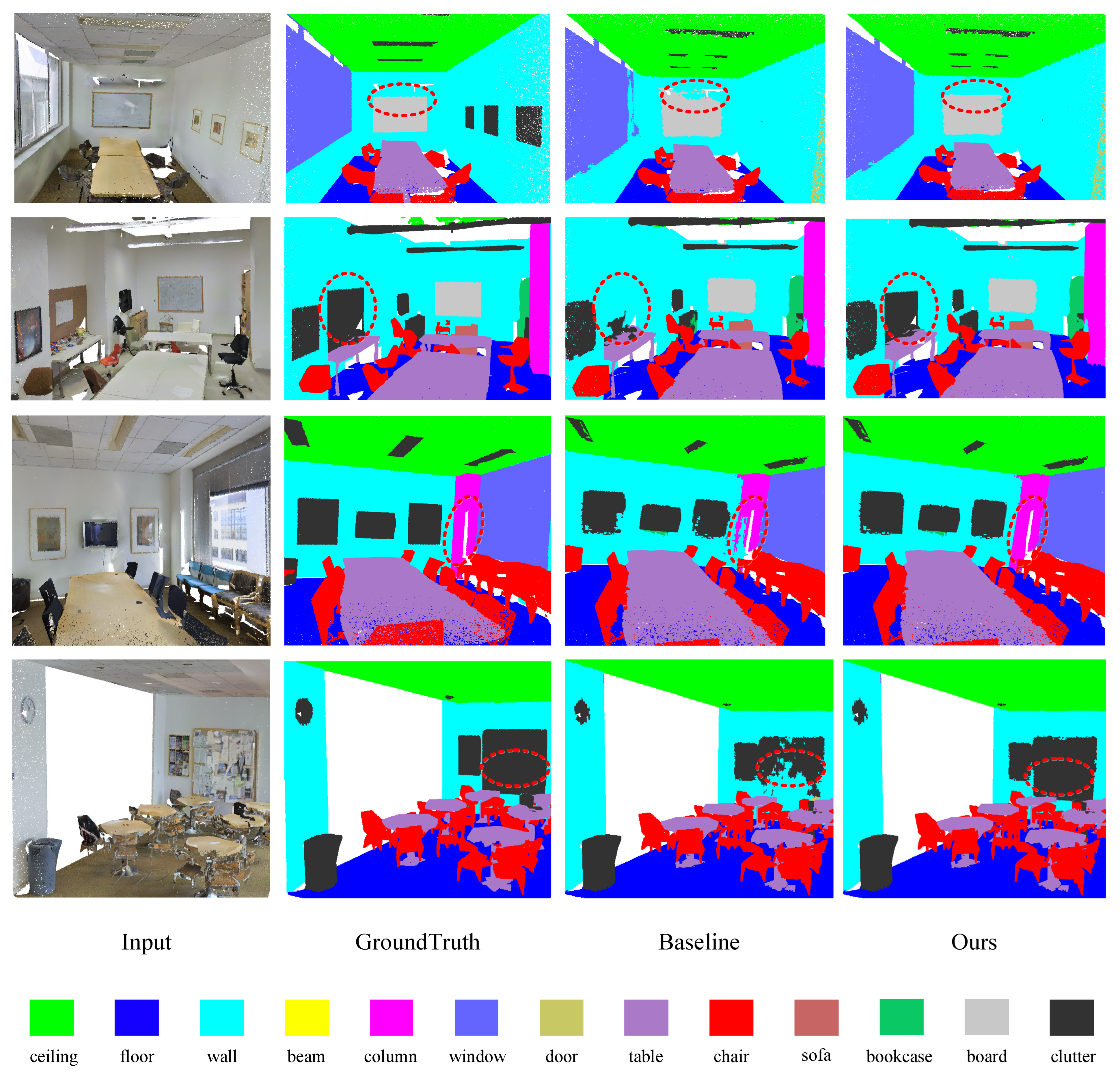
Officially, the scenes from Area 5 of S3DIS were used for testing. The qualitative improvements of our method on boundary regions are highlighted by red dotted circles in Figure 7. Notice that our method performed well on categories with explicit boundaries such as ceiling, floor, wall, and window. Moreover, our method not only segmented boundaries precisely but also enhanced the overall performance by a large margin from the baseline. As shown in Table 3, the overall accuracy (OA), the mean accuracy, and the mean intersection over union (mIoU) were considered to compare the performance of our method with some recent remarkable networks. As a whole, our method presented a compelling segmentation result with the help of our boundary-aware network.
For the generality of the experiment results, we also conducted a sixfold cross-validation (Table 4) by changing the testing area in turn. Our method outperformed previous methods with leading results on overall accuracy and the mean intersection over union (mIoU).

4.3. Transfer Learning

4.3.1. Object Classification

Point cloud classification is an important problem in 3D scene understanding. We evaluated the transfer learning performance of our network from the ShapeNet dataset to the ModelNet40 dataset. The ModelNet40 [59] is built from 12,311 objects covering 40 categories, with 9843 objects for training and 2468 objects for testing. In the training phase, we employed the AdamW [42] optimizer with an initial learning rate set to 0.001 and a weight decay of 0.5. The model was trained for 200 epochs and the batch size was set to 64.
To verify the effectiveness of our method in feature representation for point clouds, we transferred our network to the point cloud classification task. In particular, after we trained our network from the ShapeNet dataset, we froze the parameters of the encoder and trained a linear SVM classifier on ModelNet40. The overall accuracy (OA) results are shown in Table 5. Since the encoder and the SVM were trained on different datasets, the experiment showed the generalization ability of our network. Moreover, we also compared with other supervised methods as shown in Table 6. Initialized with the proposed pretraining method results, our method achieved an outstanding accuracy performance.
We extended our method to a real-world dataset, ScanObjectNN [67]. The dataset provides a more challenging setup than ModelNet40, considering the background and occlusions in realistic scenarios. It contains 2902 objects spread across 15 categories. The results of our proposed method and some existing excellent methods on the ScanObjectNN dataset are presented in Table 7.

4.3.2. Few-Shot Classification

To evaluate the generalization performance of our model, we conducted few-shot classification experiments on ModelNet40 dataset. We followed the standard “K-way N-shot” configuration for data generation. In the training phase, we randomly selected K categories in the training set with N samples for each category. The K × N samples constituted a support set for the model. Then, a batch of samples were selected from the remaining data of these categories as the query set to evaluate the model. We ran 10 different rounds according to the same settings and reported the mean outcome. In Table 8, we compare the result of our model with some other state-of-the-art approaches under four different data conditions. Ours-rand represents the proposed network training from scratch. Our method outperformed the Point Transformer by 0.8%/1.2%/0.6%/0.9%, which was promoted by 0.6%/0.8%/0.4%/0.7% through pretraining, demonstrating the effectiveness of our self-supervised pretraining method.

4.3.3. Object Detection

Object detection is a traditional task in the field of computer vision. Different from image recognition, 3D object detection needs to provide not only the identification and classification of objects present in the point clouds, but also the location of the object through a minimal 3D bounding box. A 3D bounding box is the smallest cuboid that encloses a target object in the real 3D world. Theoretically, a 3D bounding box has nine degrees of freedom, three for the position, three for the rotation, and three for the dimensional size. The SUNRGB-D [69] dataset is a popular densely annotated dataset for target detection, and the average precision (AP) is commonly used to evaluate the model. We combined our pretrained model with the state-of-the-art detection framework VoteNet. The AP 25 and AP 50 results are listed in Table 9; a 5.8% promotion on AP 25 indicates that our pretraining method provided benefits compared with training from scratch.

5. Discussion

5.1. Boundary Extraction Strategies

As the proposed pretraining task requires accurate boundary points as a prerequisite. Therefore, we compare the performance of the boundary extractor in the model with another two edge detection methods [76,77]. The comparison methods are referred as the discontinuity-based (D+SC) method and the eigenvalue analysis (EA) method, respectively. The ground truth of the boundary points was generated by Meshlab. A quantitative analysis of the results was performed using precision and recall estimates. As shown in Figure 8, as the recall rate increased, the accuracy of the D+SC [76] and EA [77] methods tended to decrease. In contrast, our method showed a consistently higher precision and recall, providing more precise and complete boundary proposals.

5.2. Effectiveness of the MFP Pretraining

In Table 10, we compare our pretraining method for network initialization with some recent methods including OcCo, Point-BERT, and training from scratch. We conducted experiments on ScanNet v2 and S3DIS, with the same fine-tuning strategy for each dataset. We can see that the self-supervised pretraining progress significantly raised the supervised-from-scratch baseline with the geometric priors learned from the boundary regions. In addition, our mixed feature prediction (MFP) pretraining method averted the time and space overhead for training the dVAE-based tokenizer for point clouds.
We adopted random masking and compared the influence of different mixing ratios for boundary sampling points in Table 11. Different from the masking ratios in NLP and computer vision (15% to 40%), we surprisingly found that a higher mixing ratio resulted in better performance for point cloud tasks. The reason lay in the discontinuous nature of the unorganized point clouds. The optimal masking ratio was eventually confirmed as 90% in our experiments.

5.3. Effectiveness of the DFA Module

The dynamic feature aggregation module adopted an adaptive dilated KNN search for points at different positions. With the combination of different dilated ratios, the detailed information became diverse with flexible receptive fields. Table 12 shows different arrangements for the feature extraction of the boundary regions on ScanNet v2 and S3DIS. Notably, both the features in small receptive fields and in large receptive fields were critical for boundary learning.
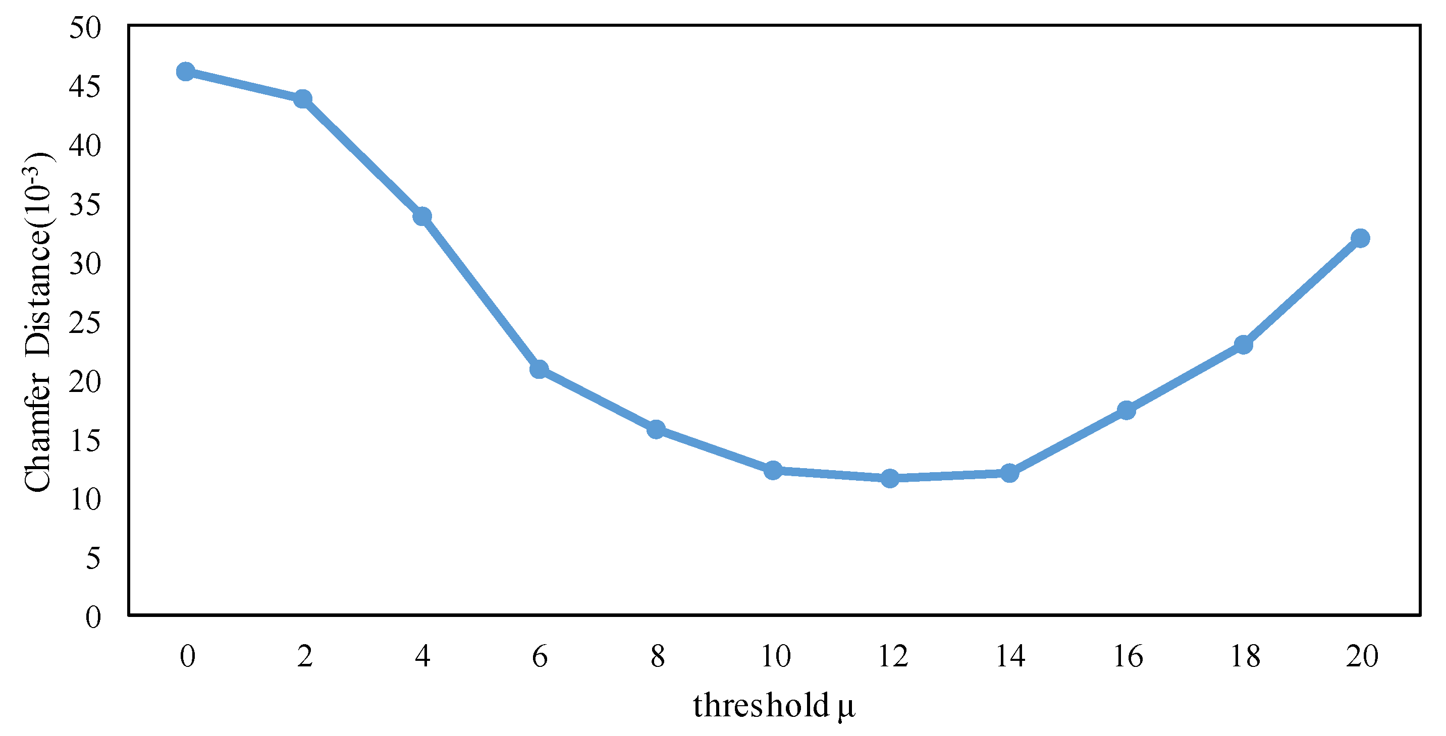
Our network was trained on 2048 points with a number of neighbors K of 20. We conducted experiments with varying values of the threshold parameter μ , from 0 to 20. The results are presented in Figure 9. As μ increased, the number of points divided into boundary regions gradually decreased. To obtain an even distributed clustering result, we eventually selected μ = 12 on ShapeNet for pretraining.

5.4. Effectiveness of the BLC Loss

The boundary label-consistent loss serves as an implicit auxiliary supervision signal for point features. It focuses on the interclass regions and differentiates the point features of each region via boundary information. After the experimental test, the weight θ of the BLC loss was set to 0.2 in our implementation. We conducted an ablation study, whose results are shown in Table 13. Equipped with the BLC-loss, 0.6% and 0.5% increases were achieved on the ScanNet v2 and S3DIS datasets, respectively.

5.5. Complexity Analysis

Finally, we compared the model complexity of our method with that of other point cloud segmentation methods. For the sake of fairness, all the experiments were performed with two paralleled RTX 2080Ti GPUs on the ModelNet40 dataset. As shown in Table 14, PointNet++ [21] and DGCNN [44] are time-consuming, a major reason being that they both adopt the computationally expensive FPS sampling operation. KPConv [22] is difficult to extend to large scenes due to its high computational and memory cost. The Point Transformer [23] suffers from a large number of parameters on account of the huge calculation required from the self-attention layer. Our method requires fewer parameters while maintaining a competitive result. Thanks to the proposed dynamic feature aggregation (DFA) method, we employed different point convolution strategies according to spatial properties for point clouds, thus allowing the proposed model to extract long-range geometric dependency with less time. Furthermore, we used the simple random sampling operation together with the efficient shared-MLPs to aggregate features, which was especially beneficial for reducing inference time.
We followed the stand-point-based processing design to build our network architecture. The detailed configuration is shown in Table 15.

6. Conclusions

Semantic segmentation technology plays a key role in extracting valuable content from large quantities of 3D data for better scene understanding. In this paper, we presented a simple and efficient framework focusing on the boundary regions for the point cloud semantic segmentation task. Through a mixed feature prediction task, the model obtained accurate boundary perception ability through pretraining. To capture local information more efficiently, we further proposed a dynamic feature aggregation (DFA) module to search for the best fitting neighbors under different receptive fields. In addition, a novel boundary label-consistent loss was integrated into our network to ensure the boundary smoothness of segmentation results. Overall, our proposed self-supervised learning method achieved results comparable with fully supervised learning in semantic segmentation tasks, avoiding the high cost of manual labeling for point clouds. On this basis, we can take advantage of large-scale raw data for training, greatly improving the applicability and robustness of neural network models in domains such as autonomous driving, augmented reality, robotics, and medical treatment. In the future, we will explore the method of integrating the information from multisource data. The texture features contained in hyperspectral remote sensing images are conducive to understanding the large-scale real-world point cloud scenarios.

Author Contributions

F.H., J.L. and R.S. conceived and designed the study; F.H. performed the experiments and analyzed the data; F.H. and J.L. wrote the paper; K.C., R.S. and Y.L. reviewed and edited the manuscript. All authors have read and agreed to the published version of the manuscript.

Funding

This research was supported in part by the Fundamental Research Funds for the Central Universities under Grant JBF22010, the National Nature Science Foundation of China under Grant 61901343, the state Key Laboratory of Geo-Information Engineering (no. SKLGIE2020-M-3-1), the science and technology on space intelligent control laboratory ZDSYS-2019-03, the China Postdoctoral Science Foundation (no. 2017M623124), the China Postdoctoral Science Special Foundation (no. 2018T111019) and the Youth Innovation Team of Shaanxi Universities. The project was also partially supported by the Open Research Fund of CAS Key Laboratory of Spectral Imaging Technology (no. LSIT201924W), and Wuhu and Xidian University special fund for industry-university-research cooperation (no. XWYCXY-012021002).

Data Availability Statement

Publicly available datasets were analyzed in this study. The datasets can be found here: http://modelnet.cs.princeton.edu/ (accessed on 5 July 2022), https://www.shapenet.org/ (accessed on 5 July 2022), http://www.scan-net.org/ (accessed on 5 July 2022), http://buildingparser.stanford.edu/(accessed on 5 July 2022), and https://rgbd.cs.princeton.edu/ (accessed on 5 July 2022).

Conflicts of Interest

The authors declare no conflict of interest. The funding sponsors had no role in the design of the study; in the collection, analyses, or interpretation of data; in the writing of the manuscript, and in the decision to publish the results.

References

  1. Jing, W.; Zhang, W.; Li, L.; Di, D.; Chen, G.; Wang, J. AGNet: An Attention-Based Graph Network for Point Cloud Classification and Segmentation. Remote Sens. 2022, 14, 1036. [Google Scholar] [CrossRef]
  2. Wan, J.; Xie, Z.; Xu, Y.; Zeng, Z.; Yuan, D.; Qiu, Q. Dganet: A dilated graph attention-based network for local feature extraction on 3D point clouds. Remote Sens. 2021, 13, 3484. [Google Scholar] [CrossRef]
  3. Lin, X.; Wang, F.; Yang, B.; Zhang, W. Autonomous vehicle localization with prior visual point cloud map constraints in gnss-challenged environments. Remote Sens. 2021, 13, 506. [Google Scholar] [CrossRef]
  4. Aldibaja, M.; Suganuma, N. Graph slam-based 2.5d lidar mapping module for autonomous vehicles. Remote Sens. 2021, 13, 5066. [Google Scholar] [CrossRef]
  5. Huang, J.; Stoter, J.; Peters, R.; Nan, L. City3D: Large-Scale Building Reconstruction from Airborne LiDAR Point Clouds. Remote Sens. 2022, 14, 2254. [Google Scholar] [CrossRef]
  6. Neuville, R.; Bates, J.S.; Jonard, F. Estimating forest structure from UAV-mounted LiDAR point cloud using machine learning. Remote Sens. 2021, 13, 352. [Google Scholar] [CrossRef]
  7. Devlin, J.; Chang, M.W.; Lee, K.; Toutanova, K. BERT: Pre-training of deep bidirectional transformers for language understanding. In Proceedings of the NAACL HLT 2019—Conference of the North American Chapter of the Association for Computational Linguistics: Human Language Technologies, Minneapolis, MN, USA, 3–5 June 2019; pp. 4171–4186. [Google Scholar]
  8. Bansal, T.; Jha, R.; Munkhdalai, T.; McCallum, A. Self-supervised meta-learning for few-shot natural language classification tasks. In Proceedings of the EMNLP—2020 Conference on Empirical Methods in Natural Language Processing, Online, 16–20 November 2020; pp. 522–534. [Google Scholar]
  9. Wei, C.; Fan, H.; Xie, S.; Wu, C.Y.; Yuille, A.; Feichtenhofer, C. Masked Feature Prediction for Self-Supervised Visual Pre-Training. arXiv 2021, arXiv:2112.09133. [Google Scholar]
  10. Xie, Z.; Zhang, Z.; Cao, Y.; Lin, Y.; Bao, J.; Yao, Z.; Dai, Q.; Hu, H. SimMIM: A Simple Framework for Masked Image Modeling. arXiv 2021, arXiv:2111.09886. [Google Scholar]
  11. Yu, X.; Tang, L.; Rao, Y.; Huang, T.; Zhou, J.; Lu, J. Point-BERT: Pre-training 3D Point Cloud Transformers with Masked Point Modeling. arXiv 2021, arXiv:2111.14819. [Google Scholar]
  12. He, K.; Chen, X.; Xie, S.; Li, Y.; Dollár, P.; Girshick, R. Masked Autoencoders Are Scalable Vision Learners. arXiv 2021, arXiv:2111.06377. [Google Scholar]
  13. Zhao, Y.; Birdal, T.; Deng, H.; Tombari, F. 3D point capsule networks. In Proceedings of the 2019 IEEE/CVF Conference on Computer Vision and Pattern Recognition (CVPR), Long Beach, CA, USA, 15–20 June 2019; pp. 1009–1018. [Google Scholar]
  14. Yang, Y.; Feng, C.; Shen, Y.; Tian, D. FoldingNet: Point Cloud Auto-encoder via Deep Grid Deformation. In Proceedings of the 2018 IEEE/CVF Conference on Computer Vision and Pattern Recognition, Salt Lake City, UT, USA, 18–23 June 2018; pp. 206–215. [Google Scholar]
  15. Gao, X.; Hu, W.; Qi, G.J. Graphter: Unsupervised learning of graph transformation equivariant representations via auto-encoding node-wise transformations. In Proceedings of the 2020 IEEE/CVF Conference on Computer Vision and Pattern Recognition (CVPR), Seattle, WA, USA, 13–19 June 2020; pp. 7161–7170. [Google Scholar]
  16. Generative, B.; Networks, A.; Gan, P.; Networks, G.A. Point Cloud Gan. arXiv 2018, arXiv:1810.05795. [Google Scholar]
  17. Vosselman, G.; Gorte, B.G.H.; Sithole, G.; Rabbani, T. Recognising structure in laser scanner point clouds. Int. Arch. Photogramm. Remote Sens. Spat. Inf. Sci. 2004, 46, 33–38. [Google Scholar]
  18. Rabbani, T.; van den Heuvel, F.a.; Vosselman, G. Segmentation of point clouds using smoothness constraint. Remote Sens. Spat. Inf. Sci. 2006, 36, 248–253. [Google Scholar]
  19. Jagannathan, A.; Miller, E.L. Three-dimensional surface mesh segmentation using curvedness-based region growing approach. IEEE Trans. Pattern Anal. Mach. Intell. 2007, 29, 2195–2204. [Google Scholar] [CrossRef]
  20. Qi, C.R.; Su, H.; Mo, K.; Guibas, L.J. PointNet: Deep learning on point sets for 3D classification and segmentation. In Proceedings of the 2017 IEEE Conference on Computer Vision and Pattern Recognition (CVPR), Honolulu, HI, USA, 21–26 July 2017; pp. 77–85. [Google Scholar]
  21. Qi, C.R.; Yi, L.; Su, H.; Guibas, L.J. PointNet++: Deep hierarchical feature learning on point sets in a metric space. In Proceedings of the 31st NIPS’17 International Conference on Neural Information Processing Systems, Long Beach, CA, USA, 4–9 December 2017; pp. 5100–5109. [Google Scholar]
  22. Thomas, H.; Qi, C.R.; Deschaud, J.E.; Marcotegui, B.; Goulette, F.; Guibas, L. KPConv: Flexible and deformable convolution for point clouds. In Proceedings of the 2019 IEEE/CVF International Conference on Computer Vision (ICCV), Seoul, Korea, 27 October–2 November 2019; pp. 6410–6419. [Google Scholar]
  23. Engel, N.; Belagiannis, V.; Dietmayer, K. Point Transformer. IEEE Access 2021, 9, 26–40. [Google Scholar] [CrossRef]
  24. Yu, X.; Rao, Y.; Wang, Z.; Liu, Z.; Lu, J.; Zhou, J. PoinTr: Diverse Point Cloud Completion with Geometry-Aware Transformers. In Proceedings of the 2021 IEEE/CVF International Conference on Computer Vision (ICCV), Montreal, QC, Canada, 10–17 October 2021; pp. 12478–12487. [Google Scholar]
  25. Guo, M.H.; Cai, J.X.; Liu, Z.N.; Mu, T.J.; Martin, R.R.; Hu, S.M. PCT: Point cloud transformer. Comput. Vis. Media 2021, 7, 187–199. [Google Scholar] [CrossRef]
  26. Zhou, P.; Zhang, D.; Cheng, G.; Han, J. Weakly Supervised Learning for Target Detection in Remote Sensing Images. IEEE Geosci. Remote Sens. Lett. 2015, 12, 318–323. [Google Scholar]
  27. Wan, Y.; Zhao, Q.; Guo, C.; Xu, C.; Fang, L. Multi-Sensor Fusion Self-Supervised Deep Odometry and Depth Estimation. Remote Sens. 2022, 14, 1228. [Google Scholar] [CrossRef]
  28. Li, X.; Liu, S.; Kim, K.; Mello, S.D.; Jampani, V.; Mar, C.V. Self-supervised Single-view 3D Reconstruction via Semantic Consistency. arXiv 2020, arXiv:2003.06473v1. [Google Scholar]
  29. Li, Y.; Li, K.; Jiang, S.; Zhang, Z.; Huang, C.; Da Xu, R.Y. Geometry-driven self-supervised method for 3D human pose estimation. In Proceedings of the AAAI 2020—34th AAAI Conference on Artificial Intelligence, New York, NY, USA, 7–12 February 2020; pp. 11442–11449. [Google Scholar]
  30. Eckart, B.; Yuan, W.; Liu, C.; Kautz, J. Self-Supervised Learning on 3D Point Clouds by Learning Discrete Generative Models. In Proceedings of the 2021 IEEE/CVF Conference on Computer Vision and Pattern Recognition (CVPR), Nashville, TN, USA, 20–25 June 2021; pp. 8244–8253. [Google Scholar]
  31. Tang, L.; Zhan, Y.; Chen, Z.; Yu, B.; Tao, D. Contrastive Boundary Learning for Point Cloud Segmentation. In Proceedings of the IEEE Computer Society Conference on Computer Vision and Pattern Recognition, New Orleans, LA, USA, 19–24 June 2022. [Google Scholar]
  32. Sauder, J.; Sievers, B. Self-supervised deep learning on point clouds by reconstructing space. arXiv 2019, arXiv:1901.08396. [Google Scholar]
  33. Noroozi, M.; Favaro, P. Unsupervised learning of visual representations by solving jigsaw puzzles. In Proceedings of the European Conference on Computer Vision; Springer: Cham, Switzerland, 2016; Volume 9910, pp. 69–84. [Google Scholar]
  34. Li, X.; Li, X.; Zhang, L.; Cheng, G.; Shi, J.; Lin, Z.; Tan, S.; Tong, Y. Improving Semantic Segmentation via Decoupled Body and Edge Supervision. In Proceedings of the European Conference on Computer Vision; Springer: Cham, Switzerland, 2020; Volume 12362, pp. 435–452. [Google Scholar]
  35. Zhen, M.; Wang, J.; Zhou, L.; Li, S.; Shen, T.; Shang, J.; Fang, T.; Quan, L. Joint semantic segmentation and boundary detection using iterative pyramid contexts. In Proceedings of the 2020 IEEE/CVF Conference on Computer Vision and Pattern Recognition (CVPR), Seattle, WA, USA, 13–19 June 2020; pp. 13663–13672. [Google Scholar]
  36. Yu, L.; Li, X.; Fu, C.W.; Cohen-Or, D.; Heng, P.A. EC-Net: An edge-aware point set consolidation network. In Proceedings of the European Conference on Computer Vision; Springer: Cham, Switzerland, 2018; pp. 398–414. [Google Scholar]
  37. Jiang, L.; Zhao, H.; Liu, S.; Shen, X.; Fu, C.W.; Jia, J. Hierarchical point-edge interaction network for point cloud semantic segmentation. In Proceedings of the 2019 IEEE/CVF International Conference on Computer Vision (ICCV), Seoul, Korea, 27 October–2 November 2019; pp. 10432–10440. [Google Scholar]
  38. Hu, Z.; Zhen, M.; Bai, X.; Fu, H.; lan Tai, C. JSENet: Joint Semantic Segmentation and Edge Detection Network for 3D Point Clouds. In Proceedings of the European Conference on Computer Vision; Springer: Cham, Switzerland, 2020; Volume 12365, pp. 222–239. [Google Scholar]
  39. Zhang, J.; Chen, L.; Ouyang, B.; Liu, B.; Zhu, J.; Chen, Y.; Meng, Y.; Wu, D. PointCutMix: Regularization Strategy for Point Cloud Classification. arXiv 2021, arXiv:2101.01461. [Google Scholar] [CrossRef]
  40. Deng, Q.; Zhang, S.; DIng, Z. Point Cloud Resampling via Hypergraph Signal Processing. IEEE Signal Process. Lett. 2021, 28, 2117–2121. [Google Scholar] [CrossRef]
  41. Chang, A.X.; Funkhouser, T.; Guibas, L.; Hanrahan, P.; Huang, Q.; Li, Z.; Savarese, S.; Savva, M.; Song, S.; Su, H.; et al. ShapeNet: An Information-Rich 3D Model Repository. arXiv 2015, arXiv:1512.03012. [Google Scholar]
  42. Loshchilov, I.; Hutter, F. Decoupled weight decay regularization. In Proceedings of the 7th International Conference on Learning Representations, ICLR, New Orleans, LA, USA, 6–9 May 2019. [Google Scholar]
  43. Yi, L.; Kim, V.G.; Ceylan, D.; Shen, I.C.; Yan, M.; Su, H.; Lu, C.; Huang, Q.; Sheffer, A.; Guibas, L. A scalable active framework for region annotation in 3D shape collections. ACM Trans. Graph. 2016, 35, 1–12. [Google Scholar] [CrossRef]
  44. Wang, Y.; Sun, Y.; Liu, Z.; Sarma, S.E.; Bronstein, M.M.; Solomon, J.M. Dynamic graph Cnn for learning on point clouds. ACM Trans. Graph. 2019, 38, 1–2. [Google Scholar] [CrossRef]
  45. Li, Y.; Bu, R.; Sun, M.; Wu, W.; Di, X.; Chen, B. PointCNN: Convolution on X-transformed points. arXiv 2018, arXiv:1801.07791v5. [Google Scholar]
  46. Liu, Y.; Fan, B.; Xiang, S.; Pan, C. Relation-shape convolutional neural network for point cloud analysis. In Proceedings of the 2019 IEEE/CVF Conference on Computer Vision and Pattern Recognition (CVPR), Long Beach, CA, USA, 15–20 June 2019; pp. 8887–8896. [Google Scholar]
  47. Lei, H.; Akhtar, N.; Mian, A. Spherical Kernel for Efficient Graph Convolution on 3D Point Clouds. IEEE Trans. Pattern Anal. Mach. Intell. 2021, 43, 3664–3680. [Google Scholar] [CrossRef]
  48. Dai, A.; Chang, A.X.; Savva, M.; Halber, M.; Funkhouser, T.; Nießner, M. ScanNet: Richly-annotated 3D reconstructions of indoor scenes. In Proceedings of the 2017 IEEE Conference on Computer Vision and Pattern Recognition (CVPR), Honolulu, HI, USA, 21–26 July 2017; pp. 2432–2443. [Google Scholar]
  49. Wu, W.; Qi, Z.; Fuxin, L. PointCONV: Deep convolutional networks on 3D point clouds. In Proceedings of the 2019 IEEE/CVF Conference on Computer Vision and Pattern Recognition (CVPR), Long Beach, CA, USA, 15–20 June 2019; pp. 9613–9622. [Google Scholar]
  50. Wang, P.S.; Liu, Y.; Guo, Y.X.; Sun, C.Y.; Tong, X. O-CNN: Octree-based convolutional neural networks for 3D shape analysis. ACM Trans. Graph. 2017, 36, 1–11. [Google Scholar] [CrossRef] [Green Version]
  51. Choy, C.; Gwak, J.; Savarese, S. 4D spatio-temporal convnets: Minkowski convolutional neural networks. In Proceedings of the 2019 IEEE/CVF Conference on Computer Vision and Pattern Recognition (CVPR), Long Beach, CA, USA, 15–20 June 2019; pp. 3070–3079. [Google Scholar]
  52. Nekrasov, A.; Schult, J.; Litany, O.; Leibe, B.; Engelmann, F. Mix3D: Out-of-Context Data Augmentation for 3D Scenes. In Proceedings of the 2021 International Conference on 3D Vision (3DV), London, UK, 1–3 December 2021; pp. 116–125. [Google Scholar]
  53. Armeni, I.; Sener, O.; Zamir, A.R.; Jiang, H.; Brilakis, I.; Fischer, M.; Savarese, S. 3D semantic parsing of large-scale indoor spaces. In Proceedings of the 2016 IEEE Conference on Computer Vision and Pattern Recognition (CVPR), Las Vegas, NV, USA, 27–30 June 2016; pp. 1534–1543. [Google Scholar]
  54. Hu, Q.; Yang, B.; Xie, L.; Rosa, S.; Guo, Y.; Wang, Z.; Trigoni, N.; Markham, A. Randla-Net: Efficient semantic segmentation of large-scale point clouds. In Proceedings of the 2020 IEEE/CVF Conference on Computer Vision and Pattern Recognition (CVPR), Seattle, WA, USA, 13–19 June 2020. [CrossRef]. [Google Scholar]
  55. Tchapmi, L.P.; Choy, C.B.; Armeni, I.; Gwak, J.; Savarese, S. SEGCloud: Semantic Segmentation of 3D Point Clouds. In Proceedings of the 2017 International Conference on 3D Vision (3DV), Qingdao, China, 10–12 October 2017; pp. 537–547. [Google Scholar]
  56. Landrieu, L.; Simonovsky, M. Large-Scale Point Cloud Semantic Segmentation with Superpoint Graphs. In Proceedings of the 2018 IEEE/CVF Conference on Computer Vision and Pattern Recognition, Salt Lake City, UT, USA, 18–23 June 2018; pp. 4558–4567. [Google Scholar]
  57. Siqi, F.; Qiulei, D.; Fenghua, Z.; Yisheng, L.; Peijun, Y.; Fei-Yue, W. SCF-Net: Learning Spatial Contextual Features for Large-Scale Point Cloud Segmentation. In Proceedings of the IEEE/CVF Conference on Computer Vision and Pattern Recognition, Nashville, TN, USA, 20–25 June 2021; pp. 14504–14513. [Google Scholar]
  58. Qiu, S.; Anwar, S.; Barnes, N. Semantic Segmentation for Real Point Cloud Scenes via Bilateral Augmentation and Adaptive Fusion. In Proceedings of the 2021 IEEE/CVF Conference on Computer Vision and Pattern Recognition (CVPR), Nashville, TN, USA, 20-25 June 2021. [CrossRef]. [Google Scholar]
  59. Wu, Z.; Song, S.; Khosla, A.; Yu, F.; Zhang, L.; Tang, X.; Xiao, J. 3D ShapeNets: A deep representation for volumetric shapes. In Proceedings of the 2015 IEEE Conference on Computer Vision and Pattern Recognition (CVPR), Boston, MA, USA, 7–12 June 2015; pp. 1912–1920. [Google Scholar]
  60. Kazhdan, M.; Funkhouser, T.; Rusinkiewicz, S. Rotation Invariant Spherical Harmonic Representation of 3D Shape Descriptors. In Proceedings of the 2003 Eurographics/ACM SIGGRAPH Symposium on Geometry Processing, Aachen, Germany, 23–25 June 2003. [Google Scholar]
  61. Wu, J.; Zhang, C.; Xue, T.; Freeman, W.T.; Tenenbaum, J.B. Learning a probabilistic latent space of object shapes via 3D generative-adversarial modeling. arXiv 2016, arXiv:1610.07584. [Google Scholar]
  62. Achlioptas, P.; Diamanti, O.; Mitliagkas, I.; Guibas, L. Learning representations and generative models for 3d point clouds. In Proceedings of the International Conference on Machine Learning, Stockholm, Sweden, 10–15 July 2018; pp. 67–85. [Google Scholar]
  63. Gadelha, M.; Wang, R.; Maji, S. Multiresolution Tree Networks for 3D Point Cloud Processing; Springer: Berlin/Heidelberg, Germany, 2018; pp. 105–122. [Google Scholar]
  64. Liu, H.; Lee, Y.J. Masked Discrimination for Self-Supervised Learning on Point Clouds. arXiv 2022, arXiv:2203.11183. [Google Scholar]
  65. Xiang, T.; Zhang, C.; Song, Y.; Yu, J.; Cai, W. Walk in the Cloud: Learning Curves for Point Clouds Shape Analysis. In Proceedings of the 2021 IEEE/CVF International Conference on Computer Vision (ICCV), Montreal, QC, Canada, 10–17 October 2021. [Google Scholar]
  66. Ma, X.; Qin, C.; You, H.; Ran, H.; Fu, Y. Rethinking Network Design and Local Geometry in Point Cloud: A Simple Residual MLP Framework. arXiv 2022, arXiv:2202.07123. [Google Scholar]
  67. Uy, M.A.; Pham, Q.H.; Hua, B.S.; Nguyen, T.; Yeung, S.K. Revisiting point cloud classification: A new benchmark dataset and classification model on real-world data. In Proceedings of the 2019 IEEE/CVF International Conference on Computer Vision (ICCV), Seoul, Korea, 27 October–2 November 2019; pp. 1588–1597. [Google Scholar]
  68. Wang, H.; Lasenby, J.; Kusner, M.J. Unsupervised Point Cloud Pre-training via Occlusion Completion. In Proceedings of the 2021 IEEE/CVF International Conference on Computer Vision (ICCV), Montreal, QC, Canada, 10–17 October 2021. [Google Scholar]
  69. Zhou, B.; Lapedriza, A.; Xiao, J.; Torralba, A.; Oliva, A. Learning Deep Features for Scene Recognition using Places Database. In Proceedings of the 27th International Conference on Neural Information Processing Systems, Montreal, QC, Canada, 8–13 December 2014; pp. 487–495. [Google Scholar]
  70. Qi, C.R.; Litany, O.; He, K.; Guibas, L. Deep hough voting for 3D object detection in point clouds. In Proceedings of the 2019 IEEE/CVF International Conference on Computer Vision (ICCV), Seoul, Korea, 27 October–2 November 2019; pp. 9276–9285. [Google Scholar]
  71. Zhang, Z.; Sun, B.; Yang, H.; Huang, Q. H3DNet: 3D Object Detection Using Hybrid Geometric Primitives. In Proceedings of the European Conference on Computer Vision; Springer: Cham, Switzerland, 2020; Volume 12357, pp. 311–329. [Google Scholar]
  72. Xie, S.; Gu, J.; Guo, D.; Qi, C.R.; Guibas, L.; Litany, O. PointContrast: Unsupervised Pre-training for 3D Point Cloud Understanding. In Proceedings of the European Conference on Computer Vision; Springer: Cham, Switzerland, 2020; Volume 12348, pp. 574–591. [Google Scholar]
  73. Zhang, Z.; Girdhar, R.; Joulin, A.; Misra, I. Self-Supervised Pretraining of 3D Features on any Point-Cloud. arXiv 2021, arXiv:2101.02691. [Google Scholar]
  74. Liu, Z.; Zhang, Z.; Cao, Y.; Hu, H.; Tong, X. Group-Free 3D Object Detection via Transformers. arXiv 2022, arXiv:2104.00678. [Google Scholar]
  75. Qi, C.R.; Chen, X.; Litany, O.; Guibas, L.J. ImVoteNet: Boosting 3D Object Detection in Point Clouds with Image Votes. In Proceedings of the 2020 IEEE/CVF Conference on Computer Vision and Pattern Recognition (CVPR), Seattle, WA, USA, 13–19 June 2020; pp. 4403–4412. [Google Scholar]
  76. Bormann, R.; Hampp, J.; Hägele, M.; Vincze, M. Fast and accurate normal estimation by efficient 3d edge detection. In Proceedings of the 2015 IEEE/RSJ International Conference on Intelligent Robots and Systems (IROS), Hamburg, Germany, 28 September–2 October 2015; pp. 3930–3937. [Google Scholar]
  77. Bazazian, D.; Casas, J.R.; Ruiz-Hidalgo, J. Fast and Robust Edge Extraction in Unorganized Point Clouds. In Proceedings of the 2015 International Conference on Digital Image Computing: Techniques and Applications (DICTA), Adelaide, SA, Australia, 23–25 November 2015; pp. 1–8. [Google Scholar]
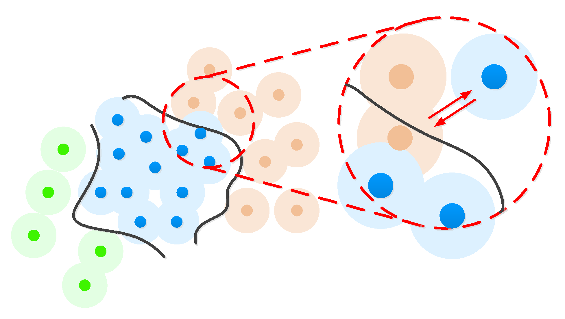
Figure 1. The boundary features are mixed by swapping the features of the boundary centroid and its farthest local neighbor.
Remotesensing 14 04757 g001
Figure 2. An overview of the proposed boundary-aware architecture for point cloud semantic segmentation. We first carry out a mixed feature prediction (MFP) task on ShapeNet to learn prior knowledge. Then, we fine-tune the network on downstream tasks based on the shared parameters. The boundary detector serves as an auxiliary supervised signal to maintain the correctness of the segmentation.
Remotesensing 14 04757 g002
Figure 3. Illustration of the mixed feature prediction task. We compare our mixed feature prediction task with the masked autoencoding workflow in the 2D image domain. The upper row shows the process to train an autoencoder by reconstructing the masked patches from the unmasked parts of the input image data. The lower row describes the main idea of an analogous method applicable to point clouds. An encoder is trained to learn sharp features of point clouds with mixed boundary feature embeddings.
Remotesensing 14 04757 g003
Figure 4. The high-frequency components that reflect sharp features in point clouds are shown in red.
Remotesensing 14 04757 g004
Figure 5. The construction of dilated neighborhood with different receptive fields for point clouds.
Remotesensing 14 04757 g005
Figure 6. The architecture of the proposed dynamic feature aggregation (DFA) module. Note that KNN denotes the dilated ratio is 1, 2KNN denotes the dilated ratio is 2, and 4KNN denotes the dilated ratio is 4. N 1 , N 2 , and N 3 denote the number of boundary points, cross points, and interior points, respectively, and N 1 + N 2 + N 3 = N .
Remotesensing 14 04757 g006
Figure 7. Qualitative comparison results on different scenes from S3DIS Area 5. Improvements on boundary regions are highlighted with red dashed circles. From left to right: the input raw point clouds, the ground-truth label, the baseline predicted results, and the predicted results of our method. The baseline represents the proposed model training from scratch, which denotes no pretraining process in the workflow.
Remotesensing 14 04757 g007
Figure 8. Precision and recall curve for the boundary extraction methods.
Remotesensing 14 04757 g008
Figure 9. Experiment conducted with varying values of the threshold parameter μ on the validation set.
Remotesensing 14 04757 g009
Table 1. Quantitative comparison with state-of-the-art methods on ShapeNet-part dataset. The bold denotes the best performance.
Methodcls.mIoU (%)int. mIoU (%)
PointNet [20]80.483.7
PointNet++ [21]81.985.1
DGCNN [44]82.385.1
PointCNN [45]84.686.1
KPConv [22]85.186.4
RS-CNN [46]84.086.2
SPH3D-GCN [47]84.986.8
PointTransformer [23]83.786.6
Point-BERT [11]84.185.6
Ours84.586.6
Table 2. Quantitative comparison with state-of-the-art methods on ScanNet v2 dataset. The bold denotes the best performance.
MethodMethodmIoU (%)
PointNet++ [21]point-based33.9
PointCNN [45]point-based45.8
PointConv [49]point-based55.6
SPH3D-GCN [47]point-based61.0
KPConv [22]point-based68.0
JSENet [38]point-based69.9
CBL [31]point-based70.5
MinkowskiNet [51]voxel-based73.6
O-CNN [50]voxel-based76.2
Mix3D [52]voxel-based78.1
Ourspoint-based75.8
Table 3. Quantitative comparison on S3DIS Area 5 dataset. Results of the overall accuracy (OA), the mean accuracy (mAcc), and the mean IoU (mIoU) are listed. The bold denotes the best performance.
MethodOA (%)mAcc (%)mIoU (%)CeilingFloorWallBeamColumnWindowDoorTableChairSofaBookcaseBoardClutter
PointNet [20] 49.041.188.897.369.80.13.946.310.859.052.65.940.326.433.2
SegCloud [55] 57.448.990.196.169.90.018.438.423.170.475.940.958.413.041.6
PointCNN [45]88.175.665.492.398.279.40.017.622.862.174.480.631.766.762.156.7
SPG [56]86.466.558.089.496.978.10.042.848.961.684.775.469.852.62.152.2
KPConv [22] 72.867.192.897.382.40.023.958.069.091.081.575.375.466.758.9
RandLA-Net [54]87.271.462.491.195.680.20.024.762.347.776.283.760.271.165.753.8
JSENet [38] 67.793.897.083.00.023.261.371.689.979.875.672.372.760.4
PT [23]90.876.570.494.098.586.30.038.063.474.389.182.474.380.276.059.3
CBL [31]90.675.269.493.998.484.20.037.057.771.991.781.877.875.669.162.9
Ours90.180.369.394.298.285.30.034.064.072.888.782.574.378.067.461.5
Table 4. Quantitative comparison of different methods on the S3DIS dataset (6-fold cross-validation). The bold denotes the best performance.
MethodOA(%)mAcc (%)mIoU (%)
PointNet++ [21]67.181.054.5
DGCNN [44]84.1-56.1
PointCNN [45]88.175.665.4
SPG [56]85.573.062.1
KPConv [22]-79.170.6
RandLA-Net [22]88.082.070.0
SCF-Net [57]88.482.771.6
BAAF [58]88.983.172.2
CBL [31]89.679.473.1
Ours90.280.773.5
Table 5. Classification results in transfer learning from ShapeNet dataset to ModelNet40 dataset. The bold denotes the best performance.
Learned Features + Linear SVMAcc (%)
SPH [60]68.2
3D-GAN [61]83.3
Latent GAN [62]85.7
MRTNet-VAE [63]86.4
FoldingNet [14]88.4
PointCapsNet [13]88.9
GraphTER [15]89.1
Ours89.3
Table 6. Comparison with other supervised methods on ModelNet40 dataset. The bold denotes the best performance.
MethodInputAcc (%)
PointNet [20]1 k89.2
PointNet++ [21]1 k90.7
DGCNN [44]1 k92.9
RS-CNN [46]1 k92.9
PointTransformer [23]-93.7
Point-BERT [11]1 k93.2
Point-MAE [64]1 k94.0
CurveNet [65]1 k94.2
PointMLP [66]1 k94.5
Ours1k94.2
Table 7. Object classification on ScanObjectNN. Three main variants were considered: object only, object with background, and the hardest perturbed variant (PB_T50_RS variant). The bold denotes the best performance.
MethodOBJ-BGOBJ-ONLYPB-T50_RS
PointNet [20]73.379.268.0
PointNet++ [21]82.384.377.9
DGCNN [44]82.886.278.1
PointCNN [45]86.185.578.5
Transformer [23]79.980.677.2
Point-BERT [11]87.488.183.1
Ours86.583.482.6
Table 8. Few-shot classification results of different methods on ModelNet40. The bold denotes the best performance.
Method5-Way10-Way
10-Shot20-Shot10-Shot20-Shot
DGCNN-rand [44]31.6 ± 2.840.8 ± 4.619.9 ± 2.116.9 ± 1.5
DGCNN-OcCo [68]90.6 ± 2.892.5 ± 1.982.9 ± 1.386.5 ± 2.2
Transformer-rand [23]87.8 ± 5.293.3 ± 4.384.6 ± 5.589.4 ± 6.3
Transformer-OcCo [68]94.0 ± 3.695.9 ± 2.389.4 ± 5.192.4 ± 4.6
Point-BERT [11]94.6 ± 3.196.3 ± 2.791.0 ± 5.492.7 ± 5.1
PointMAE [64]96.3 ± 2.597.8 ± 1.892.6 ± 4.195.0 ± 3.0
Ours-rand93.1 ± 3.294.2 ± 2.490.2 ± 3.992.3 ± 3.2
Ours96.5 ± 2.197.2 ± 2.393.1 ± 3.795.2 ± 4.1
Table 9. Transfer learning based on state-of-the-art detection frameworks. The bold denotes the best performance.
MethodSUNRGB-D
AP 25 AP 50
Frustum PointNet [66]54.0-
VoteNet [70]57.732.9
H3DNet [71]60.139.0
PointContrast [72]57.534.8
DepthConstrast [73]61.635.5
GroupFree3D [74]63.045.2
ImVoteNet [75]63.4-
Ours63.544.7
Table 10. Ablation studies on our proposed MFP pretraining method. The bold denotes the best performance.
InitializationScanNet v2 (mIoU)S3DIS (mIoU)
Supervised from scratch70.262.7
Ours-OcCo73.368.6
Ours-discrete token74.669.2
Ours-MFP75.871.4
Table 11. Mask ratio selection. The bold denotes the best performance.
Ratio20%40%60%80%90%95%
OA (%)89.190.692.993.994.293.7
Table 12. Ablation studies on the proposed DFA module. The bold denotes the best performance.
Dilate Ratio dNumber of Neighbors KScanNet v2 (mIoU)S3DIS (mIoU)
12074.567.6
22072.367.1
42061.263.3
1, 22075.670.6
2, 42075.369.3
1, 2, 42075.871.4
Table 13. Ablation studies on the proposed BLC loss. The bold denotes the best performance.
DatasetScanNet v2 (mIoU)S3DIS (mIoU)
Without BLC Loss75.270.9
With BLC Loss75.8 (↑ 0.6)71.4 (↑ 0.5)
Table 14. Complexity Analysis. The bold denotes the best performance.
MethodInputParamsForward TimeOA (%)
PointNet [20]1 k3.50 M13.2 ms89.2
PointNet++ [21]1 k1.48 M34.8 ms90.7
DGCNN [44]1 k1.81 M86.2 ms92.9
KPConv [22]1 k14.3 M33.5 ms92.9
RS-CNN [46]1 k1.41 M30.6 ms93.6
Point Transformer [23]1 k2.88 M79.6 ms93.7
Ours1 k0.88 M22.4 ms94.2
Table 15. Network architecture details. N 1 , N 2 , and N 3 denote the number of boundary points, cross points, interior points and N 1 + N 2 + N 3 = N .
ModuleBlockCinCmiddleCoutNout
DFA encoderMLP13(64, 64, 128)768 N 1
MLP23(64, 64, 128)768 N 2
MLP33(64, 64, 128)768 N 3
MaxPoolingN-1-
MFP decoderMLP768(512, 256,128)12864
Linear12864264
Segmentation headMLP387384 × 438464
EdgeConv384-512128
EdgeConv512-384128
EdgeConv384-512256
EdgeConv512-384256
EdgeConv384-512512
EdgeConv512-384512
EdgeConv384-5122048
EdgeConv512-3842048
Classficiation headMLP768(512, 256)40-
Target detection headVoting layer256256259-
Proposal layer128(128, 128)79-
Publisher’s Note: MDPI stays neutral with regard to jurisdictional claims in published maps and institutional affiliations.