Article

Virtual Laser Scanning Approach to Assessing Impact of Geometric Inaccuracy on 3D Plant Traits

1
Leibniz Institute of Plant Genetics and Crop Plant Research (IPK), D-06466 Seeland, Germany
2
Plant Sciences Core Facility, Central European Institute of Technology (CEITEC), Masaryk University, 62500 Brno, Czech Republic
*
Author to whom correspondence should be addressed.
Remote Sens. 2022, 14(19), 4727; https://doi.org/10.3390/rs14194727
Submission received: 13 August 2022 / Revised: 1 September 2022 / Accepted: 14 September 2022 / Published: 21 September 2022
(This article belongs to the Special Issue 3D Modelling and Mapping for Precision Agriculture)

Abstract

:
In recent years, 3D imaging became an increasingly popular screening modality for high-throughput plant phenotyping. The 3D scans provide a rich source of information about architectural plant organization which cannot always be derived from multi-view projection 2D images. On the other hand, 3D scanning is associated with a principle inaccuracy by assessment of geometrically complex plant structures, for example, due the loss of geometrical information on reflective, shadowed, inclined and/or curved leaf surfaces. Here, we aim to quantitatively assess the impact of geometrical inaccuracies in 3D plant data on phenotypic descriptors of four different shoot architectures, including tomato, maize, cucumber, and arabidopsis. For this purpose, virtual laser scanning of synthetic models of these four plant species was used. This approach was applied to simulate different scenarios of 3D model perturbation, as well as the principle loss of geometrical information in shadowed plant regions. Our experimental results show that different plant traits exhibit different and, in general, plant type specific dependency on the level of geometrical perturbations. However, some phenotypic traits are tendentially more or less correlated with the degree of geometrical inaccuracies in assessing 3D plant architecture. In particular, integrative traits, such as plant area, volume, and physiologically important light absorption show stronger correlation with the effectively visible plant area than linear shoot traits, such as total plant height and width crossover different scenarios of geometrical perturbation. Our study addresses an important question of reliability and accuracy of 3D plant measurements and provides solution suggestions for consistent quantitative analysis and interpretation of imperfect data by combining measurement results with computational simulation of synthetic plant models.

1. Introduction

In the last two decades, image-based assessment of phenotypic traits became an indispensable tool in quantitative plant biology [1]. Due to geometrical complexity and dynamic nature of developing plant structures, image-based estimation of even very basic plant traits, such as plant biomass, renders a challenging technical and analytical task [2].
The early approaches to plant phenotyping based on 2D projectional multi-view (i.e., rotational side and top) images enable estimation of a wide range of traits, including some proxies of 3D plant morphology, such as quasi-volume [3]. However, in general, they do not allow to accurately segment single leaves or compute such important physiological traits as light interception area and real 3D biomass that are naturally derivable from 3D data.
To quantitatively assess 3D plant organization a number of different 3D scanning and geometry reconstruction methods were developed [4,5]. The methods for 3D plant reconstruction includes laser scanning (LS) [6,7,8], stereo vision (SV) or structure from motion (SfM) [9,10,11,12,13,14], structured light (SL) [15,16,17], space/volume carving [18], time of flight (ToF) [19,20], light field (LF) [21], and terrestrial laser scanning (TLS) or Light Detection And Ranging (LIDAR) [22,23,24,25]. Despite different methodological approaches, all methods of 3D object reconstruction provide similar representation of 3D reconstructed objects in form of point clouds and/or triangulated surface meshes. In previous works, a number of methods for processing, segmentation, and analysis of 3D plant models resulting from 3D scanning or image-based 3D reconstruction was presented [26,27,28]. However, the accuracy of plant models resulting from 3D scanning and its impact on phenotypic plant traits was rarely addressed in the past.
Goldbach et al. [29] performed evaluation of their volume carving approach by comparing traits assessed from 3D reconstruction vs. manually cut individual leaves of tomato seedlings with a relatively sparse shoot architecture. Zhou et al. [30] investigated the accuracy of their greenhouse SfM imagery system on dummy objects. Amador et al. [31] presented a study on generation of point cloud models of five different plant types using the laser scanning system calibrated on synthetic geometric objects (sphere, cube, cylinder). A general approach to evaluation of accuracy of 3D scanning vs. ground truth models of arbitrary plant species, and, therefore, architectures are missing.
In this study, we present a general framework for virtual laser scanning of synthetic 3D plant models which was applied to four different plants architectures (including tomato, maize, cucumber, and arabidopsis shoots) with the goal to address the following basic questions:
  • To what extent progressive inaccuracy of 3D plant reconstruction simulated by different types of geometric noise affects the resulting 3D plant traits?
  • Can partially inaccurate measurements of 3D plant traits provide consistent quantitative description of plant morphology and physiology by combining them with the results of computational simulations of synthetic plant models?
The manuscript is structured as follows. In the next section, our methodological framework for virtual laser scanning and phenotyping of synthetic 3D plant models is described. Then, the experimental results of our simulation studies with four different 3D shoot models are presented. Finally, possible approaches to normalization of 3D plant traits derived from partial and error-afflicted measurements are discussed.

2. Methods

2.1. Modelling Platform

The modelling and simulation of this study are performed using the open-source modelling platform GroIMP v1.6 [32]. GroIMP is a widely applied plant modelling environment which is mainly used for applications in functional-structural plant modelling. It provides a rich set of features suitable for the need of this invention. In addition to a fully 3D modelling environment, it includes advanced capabilities for light modelling based on a forward Monte Carlo path tracer [33,34]. GroIMP further provides a virtual laser scanner, that allows virtually simulate 3D scans of a virtual scene. The virtual laser scanner was used to perform point-wise sample of synthetic 3D plant shoot models.

2.2. Synthetic Plant Models

Synthetic 3D models of four plant shoot architectures, including tomato, maize, cucumber, and arabidopsis, were generated and used in this study in virtual laser scanning experiments, see Figure 1. A model of an adult tomato plant was chosen as example of a relatively complex plant morphology. The greenhouse cucumber model has a similar architecture as the tomato plant but with larger, closed leaves leading to a significantly higher overlapping and so self-shading effects of leaves. An adult maize plant stands exemplary for a more simple plant architecture characterized by its distinctive 2D vertical plain geometry. In contrast, the arabidopsis plant model exhibits a flat, circular, quasi-2D shape with large leaves covering the ground. All together, these four plant architectures give examples of alternative and partially contrasting 3D plant architectures that differ with respect to their morphological and physiological properties, including light absorption, leaf coverage, density, etc.
The virtual tomato plant model, as described in Zhang et al. [35], consists of 21 internodes with one leaf at each internode. The plant model has a total height of 1.7 meter and a maximal diameter of 86 centimetre. At rank four and six a panicle of tomato fruits of different ageing stages and so sizes are modelled. The original 3D plant model was taken and converted from geometric primitive objects, i.e., cylinder, spheres, and NURBS shapes, to a set of vertices (intersection points for the triangles) and faces (triangles of the triangulation)—a pure triangulation model of the original model. This step allows us to remove small parts, i.e., individual triangles, from the whole model to “cut” holes and so to simulate perturbation effects. The triangulation contains 25,674 vertices forming a total of 8558 faces (always three vertices belong to one face). All colouring and shaders have been removed during this process. Figure 2 shows screenshots of the whole tomato plant, as well as enlargements of a leaf and single leaflet.
All other plant models are constructed and transformed into triangulated meshes in the same way as described for the tomato model. Table 1 summarizes the statistics of each virtual plant model.

2.3. Simulation Scenarios

2.3.1. Virtual Laser Scanner

An in GroIMP v1.6 integrated virtual laser scanner was used to simulate a 3D plant scanning process. The laser scanner is based on the same physical-based ray tracing model as used to perform light simulations within GroIMP, see Hemmerling et al. [33] for further details. Instead of calculating light scenarios, it was modified in a way to generate point cloud models of the scanned objects independent of the optical properties of the objects or the colour of the laser ray. The virtual laser scanner allows to perform a set of standard scanning options, such as cylindrical or spherical scanning, around an object. Further scanner parameters such as opening angle of the emitted rays and dentistry are configured to match common handheld scanner systems. Figure 3 shows a side and top view of the used hemispherical scanner dome. The virtual laser scanners are arranged in layers on a virtual hemisphere, where the distance between two neighbouring scanners, horizontally and vertically, is roughly about 50 cm. The dimension of the scanner dome is set equal for all scenarios, and dimensioned so that the highest plant (maize) fits in. The main view direction of each virtual laser scanner is pointing towards the virtual centre of the scene, where the plant model is located.
In the output, the virtual laser scanner produces a set of XYZ coordinates, where each 3D point stands for one intersection point of a ray emitted by one of the virtual laser scanners and an object, i.e., triangle/face, of the scene. The resulting point clouds are saved for further processing.
The computation time for the simulation of the virtual laser scan is directly related to resolution of the defined scanner dome, i.e., the number of scanners and so the number of simulated laser rays. The average scanning time for the tomato model is about 9.3 s while for relatively simple architectures as the arabidopsis model only 9.0 s are required on a Intel© Core™ i7-4710MQ CPU @ 2.50 GHz × 4 with 32 GB RAM.

2.3.2. Light Simulation

In addition to the simulation of the virtual laser scanner, the estimation of light absorption of the 3D structure was used as further indicator to quantify the “completeness” of the structure when compared to the original plant structure. The GroIMP in-built raytracer called “Twilight”, a bidirectional path tracer [33], was used to simulate the light scenario within the virtual 3D scene and so for the plant structures. The diffuse colour of the plant was set to pure green (RGB: 0, 255, 0), which means that all green part of light was reflected and all other parts of the visual light waveband are absorbed. The transparency of all leaves was set equally to 10 %, allowing 10 % of the incoming radiation to pass through the leaf. To generate a homogeneous, diffuse light distribution, a virtual hemisphere of 72 regularly arranged direct light sources (six circles with 12 light sources each) was used as described in [36,37]. The intensity of the total power to the diffuse sky was set constant to 1000 W for all simulations. Please note that the value of the power of the light sources does not have any effect on the observed light distribution itself or on the following absorption by individual plant organs, and can be therefore chosen arbitrarily. Changing the power can be compared to dimming a lamp, it changes only the intensity but not the overall distribution. To be able to simulate a reproducible and accurate light distribution the light model was configured to use 10 million light rays and a recursion depth of 10 reflections levels, what is more than sufficient relative to the size of the simulated 3D scene [34].
As output of the light simulation, the absorption for each face as well as the object identification number are saved.
The computation time for the light simulation is directly related to the complexity and the size of the 3D scene as well as the number of objects within the scene and the number of used light rays and their maximal recursion depth. The average light simulation time for the tomato model is about 20.8 s and about 9.3 s area required for the arabidopsis model on a Intel© Core™ i7-4710MQ CPU @ 2.50 GHz × 4 with 32 GB RAM.

2.3.3. Geometrical Perturbation Scenarios and Simulations

In this study, three thinning, or perturbation, scenarios assuming three different ways of how and where parts of the plant are lost, have been investigated, namely, random, from outside to inside (outside-to-inside), and from inside to outside (inside-to-outside). Although, in the random scenario, facets are removed randomly, for the other two scenarios, directional pattern of face elimination, i.e., from the plant periphery to stem (outside-to-inside) and in the opposite direction (inside-to-outside) is used.
For each thinning scenario, 30 simulations are performed, while at each step the plant model, or more precisely the triangulated mesh of the plant model, is reduced by one percentage of the faces starting with the complete plant. For each simulation step, the point cloud is generated by the virtual laser scanner, and the amount of absorbed light, calculated by the light model, of the reaming structure is stored for further analyses.
Figure 4 shows the effect of all three thinning scenarios at the thinning of 30 % in top view of the tomato plant model.

2.3.4. Data Analysis

Virtual laser scans of original and progressively thinned 3D plant models were subsequently analysed to calculate quantitative traits of 3D plant architecture. For each thinning step, one percentage of the initial number or faces for the complete pant was removed. For the remaining plant structure, the following features are calculated:
  • Height. Total plant height in metre defined as highest Z-coordinate of the point cloud above the ground.
  • PCA1. The length of the largest PCA axis of the scanned point cloud in [m].
  • PCA2. The length of the smallest PCA axis of the scanned point cloud in [m]. ize Convex_Hull_Volume. The 3D volume [m 3 ] of the convex hull (Figure 5) enclosing all points of the scanned point cloud.
  • Plant_AbsorbedRadiation. Total amount of radiation absorbed by the plant structure in Watt [W].
  • Plant_SurfaceArea. Total surface area [m 2 ] of the plant structure, computed as a sum of areas of all single-side faces.
  • Visible_Plant_SurfaceArea. The visible surface area [m 2 ] is defined as the sum of areas all single-side faces that are “visible” to the virtual laser scanner and obtained an intersection with at least one virtual light ray emitted by the scanner.
  • Number_ScanPoints. Total number of scanner points, i.e., number of points within the point cloud, generated by the virtual laser scanner.
Quantitative analysis of the above descriptors and, in particular, linear correlation between the quantitative traits and the visible plant area were performed using MATLAB R2021a (Mathworks Inc., Natick, MA, USA).

3. Experimental Results

In this study, we restrict our investigations to a meaningfully range of up to 30% loss of the original plant area. Perturbation is performed in one percent steps starting from zero to 30 % in number of faces, respectively, starting from a full, un-perturbed model containing all faces going down to a model that only contains 70 % of the original number of faces.
Thirty percent represent already quite a substantial loss of plant area but can be reached in real measurements thinking of dense plant architectures where inner plant parts are in the shade of outer parts.
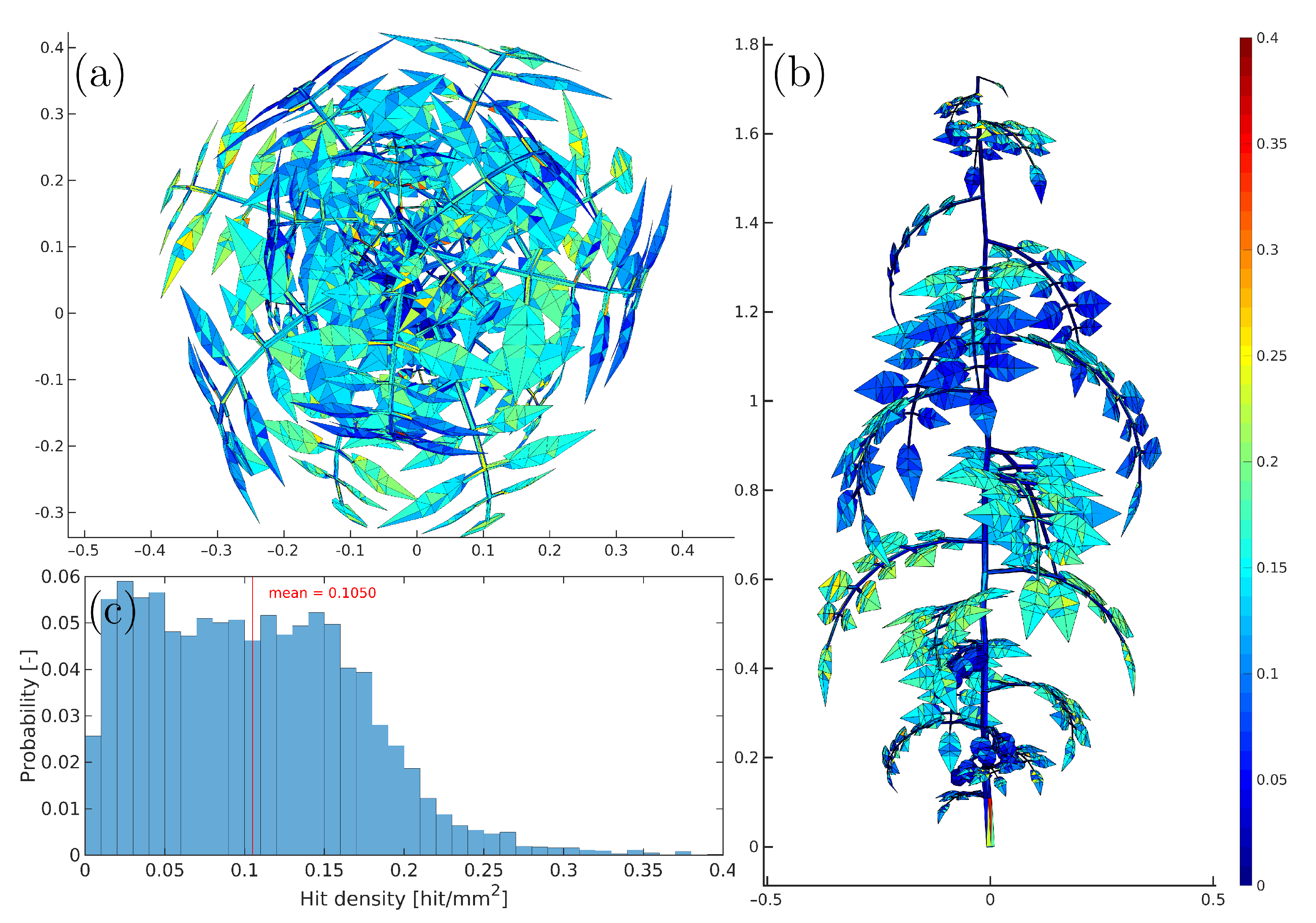
Figure 6 shows the average hit density of each triangle of the original virtual tomato model. The local hit density was calculated as a number of ray intersections (hits) with a triangle, and the average hit density per mm 2 as the average of number of hits per square millimeter of the surface area. A slightly darker blue colour in the inner areas of the plant directly visualize the lower hit density of small and very small triangles as found in the approximation of the of the internodien and petiole. This further illustrates the direct influence of outer layer of leaves that are covering the inner parts of the plant, preventing the laser rays from penetrating the plant architecture deeper and, therefore, from obtaining a complete scan. A common effect which can be seen in real world 3D scans of plants and which can be interpreted as circumstantial evidence for the reliability of the the virtual laser scanner approach used in this study. The histogram of the hit density in Figure 6c, reveals a quite homogeneous overall distribution with an average hit density of 0.105 hits per square millimeter and a variance of 0.0042.
To estimated area of a triangle which is “visible” to the virtual laser scanner, the relation between the number of hits per triangle and their area was investigated. For this purpose, the relationship between the number of ray hits and triangle area was studied on a simplified geometrical model, i.e., a half-ellipsoid fitted to the plant dimensions. Figure 7b shows the hit density per square millimeter triangle area calculated using the half-ellipsoid model. Due to a particular (hemispherical) geometry of the ray dome and the relative proportion of the plant half-ellipsoid, a slightly higher hit density around the north pole and a belt of the half-ellipsoid is seen. The correlation between the number of hits and the area of a triangle is given in Figure 7c with a r 2 of 0.93.
Since unstructured grids are typically composed of triangles of quite different size, the statistical analysis of the hit density was performed with 10 different categories of triangle areas ranging between [ 25 ( i 1 ) , 25 i ] , i = [ 1 , 10 ] . The results of this statistical analysis are presented as box-whisker plots in Figure 8. In particular, they show the median hit density for 10 different area classes with a bin width of 25 mm 2 , from zero to a maximum area of 250 mm 2 . As one expects, the average hit density for all categories with exception of very small triangles (0–25 mm 2 ) is nearly constant. Based on this observation, an equal hit density for all triangle sizes can be assumed. To calculate the visible area of a “fully visible” triangle of each plant at each perturbation level, a mean hit density of ρ m = 0.0959 hit/mm 2 is assumed. This can also be interpreted as an average projection area of 10.43 mm 2 for a single laser ray. For further processing the visible area ( v A ) of each triangle is determined as area of the triangle (A) weighted by the relative hit density ( ρ r = ρ t / ρ m ), where the relative hit density ( ρ r ) is, in turn, calculated as actual hit density of the current triangle ρ t divided by the mean hit density of a “fully visible” triangle ρ m = 0.0959 hit/mm 2 . By weighting full triangle area with the relative hit density a more realistic assessment of the “visible” triangle area is achieved. Furthermore, a triangle is considered as visible, if more than 50 % of its total surface area is calculated as “visible area”. In Table 2, the ratios of the visible area and number of visible faces for a complete (undisturbed) plant geometry are summarized. As one can see reduced visibility of faces does not equally affect the reduction in visible area. The discrepancy can be traced back to two factors: First, the size of the “invisible” faces is relatively small compared to the faces used to build the leaves. These small faces mainly building the steam elements, internodien, peduncle, and petioles, which directly leads to the second factor, the location within the plant architecture of these small faces. As main plant supporting structure, these elements are typically found hidden within the plant structure, often covered by the outer leave foliage.
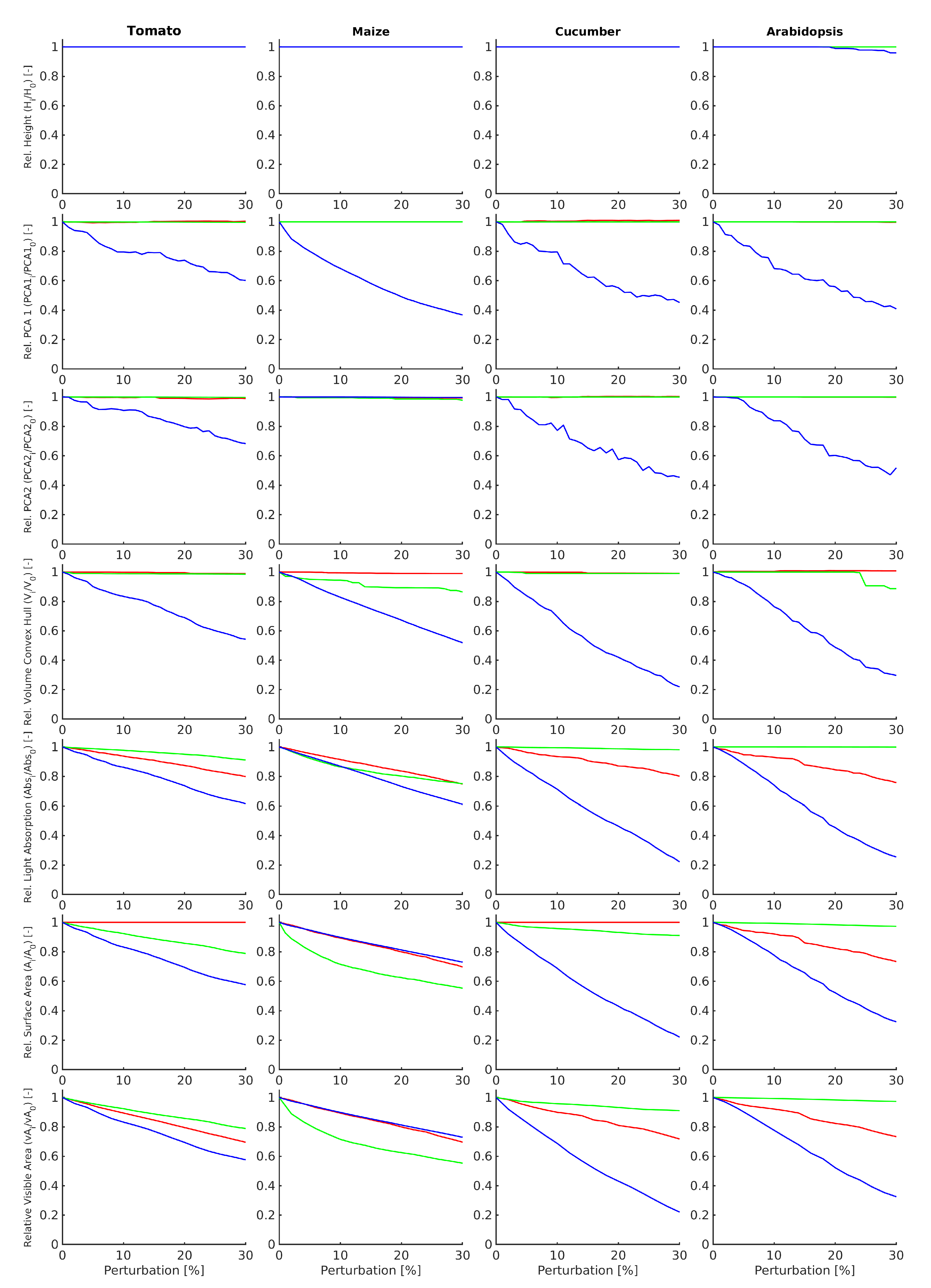
From Table 2 it is evident that only a fraction of the full-plant area is “visible” to laser scanner in all plants. However, the visible fraction of plant area depends on the plant type (i.e., 3D plant architectures) and varies in the range between 78 % for a rather more dense architecture of tomato up to 94 % for a more sparse maize and cucumber plant architecture. For every step of the geometrical model perturbation with an increment of one percent loss of faces, the above described phenotypic descriptors were calculated. In order to obtain quantitative descriptors that are independent on the absolute size of a concrete 3D model, all phenotypic traits were normalized by calculating the relative ratios to their values in the original (unperturbed) plant model, for example, H i H i / H 0 [ 0 , 1 ] , where i = 0 stands for zero (no perturbation) step of the simulation series. Figure 9 shows plots of phenotypic traits for all four plant models (tomato, maize, cucumber, and arabidopsis) and the three perturbation scenarios (random (red), outside-to-inside (blue) and inside-to-outside (green)) in dependency on the percentage of simulated area loss. From Figure 9, it is visible that that (i) some phenotypic traits are more sensitive for perturbation of 3D plant geometry than others, (ii) some perturbation scenarios exhibit stronger dependency on the loss of the visible area than other traits. In particular, the plant height is not significantly affected in all plant models and simulation scenarios for the entire range of the relative area loss from zero to 30 % . This can be attributed to the fact that the plant height is defined by a small fraction of the highest remaining points. Among all three geometrical perturbation scenarios, the outside-to-inside thinning shows the largest impact on phenotypic traits, including principle plant dimensions (PCA1 and PCA2), as well as the volume and effective light absorption, while random and inside-to-outside scenarios exhibit more moderate or no pronounced effects. This observation can be traced back to the fact that the outside-to-inside scenario has the strongest effect on the plant shape and the visible plant area compared to other two perturbation scenarios that alter the plant architecture randomly or rather hidden inner regions than are anyway covered visible leaves, and thus do not contribute significantly to quantitative traits of “visible” plant geometry. Despite the large differences between simulated plant architectures, trait responses among all four plants turn out to be remarkably comparable, although, different in their magnitude. The difference in the plant surface area between the large faces building the leaves and the relative small faces used for the supporting structure, consequently, supports the pattern seen for the outside-to-inside and inside-to-outside perturbation scenarios. Although, for the outside-to-inside scenario, first the larger faces of the leaves on the outside are remove and the remaining area decreases fast, for the inside-to-outside scenario first the relative small faces of the supporting structure are removed, leading to a relative small lost of area.
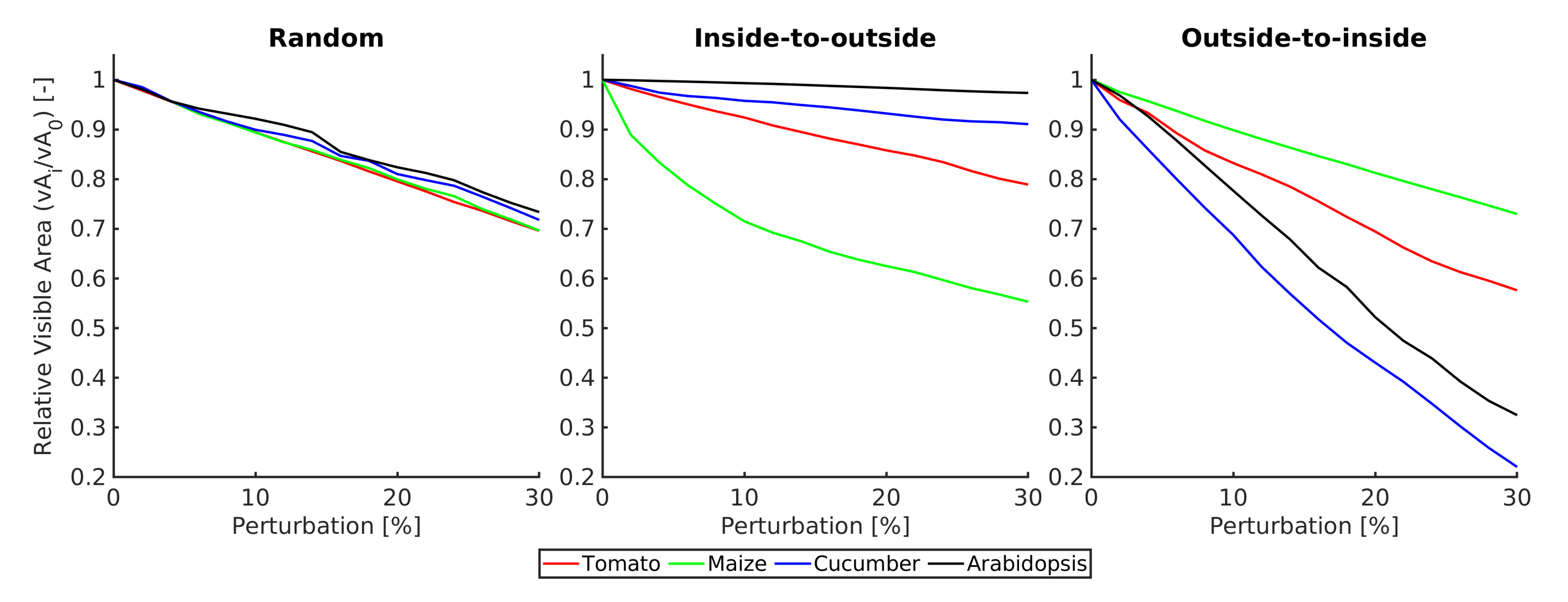
Interestingly, patterns of phenotypic traits from Figure 9 exhibit distinctive similarity to the patterns of the visible area in dependency on the geometrical loss rate shown in the last row of Figure 9. Again, the relative visible area was computed as the absolute visible area of plant leaves hit by the virtual laser rays normalized by its value in the original, i.e., unperturbed, plant model. The direct comparison of the three simulation scenarios for all four plant species shown in Figure 10 allows a more clear assessment of the effects of plant architecture on reduction in the visible area in dependency of progressive model perturbation. As one can see from this overview, random perturbation scenario affects all four plants with different spatial organization almost equally, which basically reflects the fact that random removal of faces linearly correlates with reduction in visible area. In contrast, inside-to-outside and outside-to-inside perturbations scenarios lead to different patterns of visible area reduction with progressive model perturbation. Although the maize model exhibits rapid reduction in visible area with the amount of removed faces in the inside-to-outside scenario, visible area of arabidopsis model remains almost unaffected throughout the entire range of tested perturbations of up to 30 % . By the mirrored outside-to-inside scenario, one sees the reverse pattern of visible area reduction.
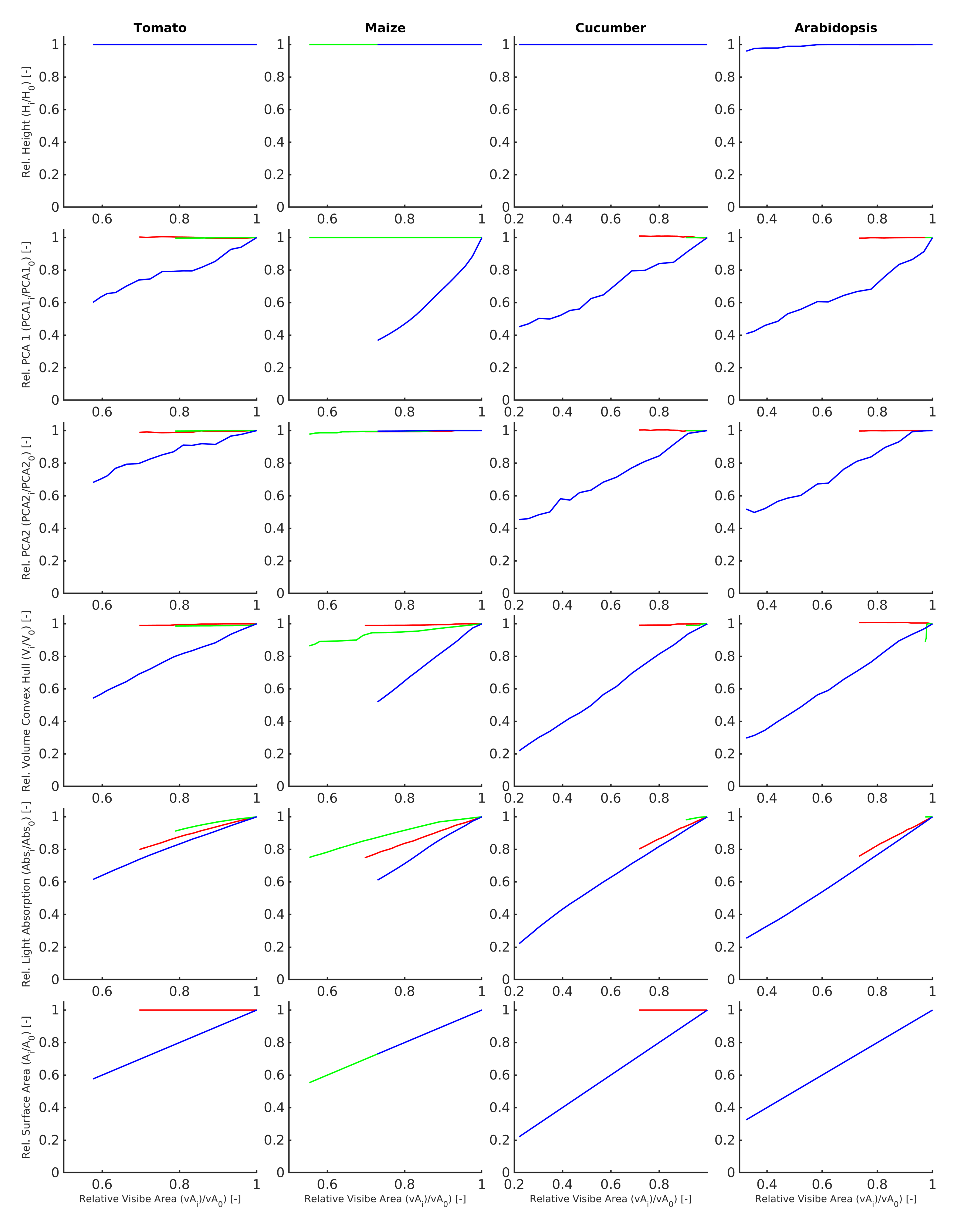
In order to dissect the relationship between the phenotypic traits and the visible plant area, all phenotypic descriptors from Figure 9 were plotted in Figure 11 vs. the relative visible area. As one can see, curves of features as function of the visible area begin now to show a clearly linear pattern. Table 3 with a summary of linear correlations between phenotypic features and the visible plant area confirms their statistically significant relationship. From Table 3, it follows that the whole plant surface area, plant volume but, in particular, also such important physiological feature as the light absorption, show a significant linear correlation with the visible plant area crossover all four plant models and three perturbation scenarios. The exact form of this functional relationship is, however, dependent on the particular plant architecture and perturbation scenario. The global features such as area and linear dimension analysed above are commonly accepted, simple descriptors of plant morphology. However, they do not allow to intrinsically assess the level of plant model perturbation especially when the perturbation scenario and degree of data loss during the measurement is not known. In order to enable a low-level analysis of shoot point cloud models, we introduced a criterion which is based on measurement of local (point-wise) smoothness. The basic idea of point cloud smoothness measurement is that the inner points are surrounded by other neighbouring points, and only regular boundary or artificial discontinuity points exhibit an asymmetric neighbourhood. To measure the local point smoothness, further termed as the smoothness factor (SF), the integral (sum) over the local neighbourhood P j ( x j , y j , z j ) of the point P i ( x i , y i , z i ) was introduced:
S F i = 1 N i = 1 N P j P i | P j P i |
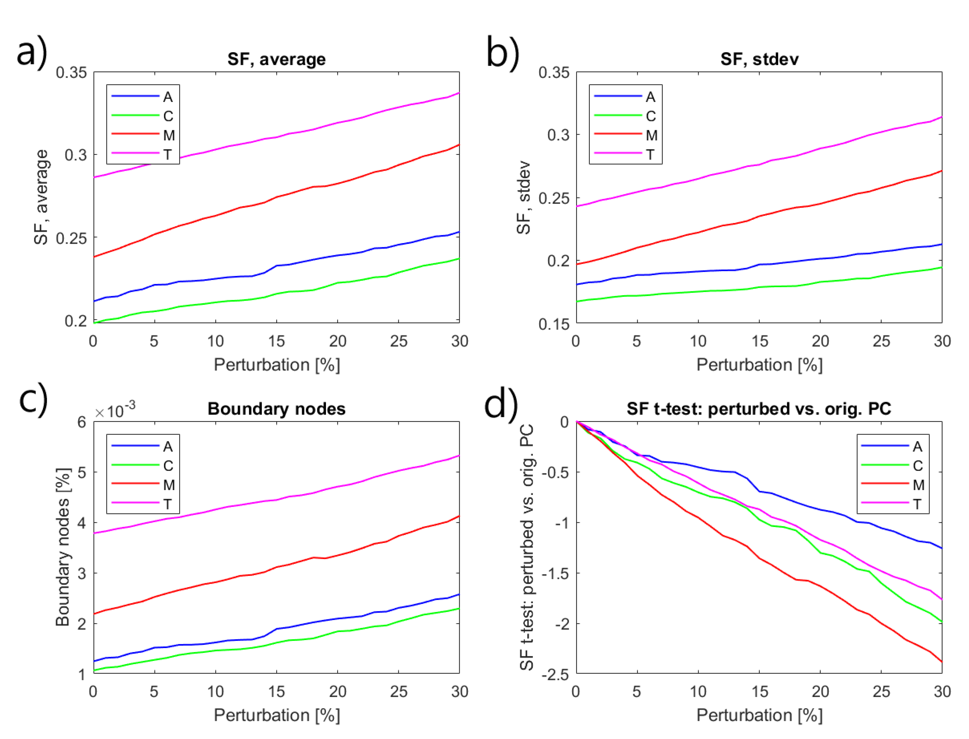
Thereby, the local neighbourhood of each and every point of the point cloud was determined using the MATLAB’s knnsearch function. The smoothness factor defined in Equation (1) takes the value zero for an inner point of a flat leaf and deviates from zero towards unity on edge and corner points. As the amount of edge and corner points growths in a geometrically perturbed (i.e., inaccurately scanned) 3D model growth, the amount of points with S F > > 0 , as well as the average SF value is expected to reflect it. Figure 12a shows the histograms of SF distributions for original (unperturbed) vs. 30 % perturbed tomato model. As one can see the distribution of SF values in a perturbed model significantly deviates from the original distribution which can be formally quantified, for examples, using the Student’s t-test between original vs. perturbed full or, in particular, boundary point cloud SF distributions. For detection of boundary points with higher SF values the threshold of SF > 0.5 was used. Figure 12b shows original vs. perturbed full and boundary point cloud models of the tomato plant. Figure 13 gives an overview of dependency of SF features on the degree of random model perturbation, including average SF, stdev of SF distributions, fraction of boundary point detected using the threshold SF > 0.5 , as well as t-test values computed from comparison of SF distributions in randomly perturbed vs. original point cloud models. As one can see all SF features show similar linear patterns of dependency on model perturbation, however, with exception of t-test values they have different starting values for different plant that obviously reflect intrinsic differences in plant architectures.

4. Conclusions

In this study, we aimed to investigate effects of geometrical inaccuracies of 3D surface scans on the resulting plant traits. For this purpose, virtual laser scanning of synthetic 3D plant models was used. Using a virtual 3D laser scanner and plant models provides us with the full control over the original pant structure, as well as the exact configuration including position and properties of the virtual laser scanner. In particular, virtual 3D scans of four different plant species (arabidopsis, cucumber, maize, and tomato) with three different scenarios of geometrical thinning/perturbation (random, outside-to-inside, and inside-to-outside) with up to 30 % loss of the total plant area were analyzed and compared. These four plants models represent four different, but common, plant architectures ranging from a complex (tomato), over large-leaf (maize) to quasi-2D rosette plant shape, such as arabidopsis. Our experimental results showed that different phenotypic traits of the whole plant geometry exhibit, in general, different responses to gradual model perturbation. Thereby, some metric features, such as, for example, the plant height turn out to be widely independent on the percentage of missing surface area, and, thus, relatively robust to inaccuracies of 3D scanning. Principle plant dimensions in the mean 2D ground projection planes (i.e., plant width, 2D projection PCA axes) are, in contrast, dependent on the type of model perturbation scenario, whereas the outside-to-inside thinning has, as expected, the strongest impact in most plant species. On the other hand, the outside-to-inside scenario turn out to be strongly dependent on the particular plant architectures which reflects in different patterns of the relative visible area reduction as a function of progressive model perturbation. In contrast, all four plant models exhibit a very similar pattern of the visible area loss in dependency on the random model perturbation. An important observation is that integrative plant features, such as the total surface area, volume of the convex plant hull, and the light absorption show a strong correlation with the visible plant area, which is the main measurable variable under real experimental conditions. This means that these integrative features can only be accurate as the visible plant area. Since this correlation was observed crossover all plant species and perturbation scenarios, normalization of features by the visible plant area would provide a widely invariant phenotypic description. The exact form of the functional dependency of phenotypic features on the visible plant area is, however, dependent on the particular plant architecture, which is typically not accessible from direct measurements, but still can be estimated using synthetic models like it was performed herein. From this viewpoint, combination of real experimental data, which is always bound to measurement of visible plant parts, with computational simulations of synthetic models of the whole plant architecture represents a promising approach to a more consistent and reliable 3D plant phenotyping.
In addition to global features of plant geometry, low-level descriptors of point cloud smoothness were studied in dependency on the degree of model perturbation. Here, we introduced a new feature termed smoothness factor (SF) which reflects the symmetry of local neighbourhood within the point cloud. Consequently, SF allows to separate inner points of a flat leaf geometry from nodes of discontinued regions, such as edges, corners, wholes, etc. Our experimental results demonstrated that conventional statistical descriptions SF distributions such such as average/stdev SF or the fraction of boundary points (related to fractal dimension) show a linear correction with the degree of model perturbation. In conjunction with re-normalization of our synthetic and real 3D scanning data, dimensionless SF features can serve as a useful measure of point cloud accuracy and consistency.
One of the main limitations of this study are an idealized (hemispherical dome) strategy of 3D scanning, as well as a rather artificial character of geometrical perturbations. The hemispherical scanner dome represents an optimal static scanner configuration to capture as much as possible of the object to be scanned. This configuration is not unusual in multi-view scanner systems. In fact, most of the stationary 3D scanning systems cover far less than the entire hemisphere around the scanned object, however, manual scanners can enable coverage of even larger perspective angles. The three perturbation scenarios simulated in this study reflect, even if extreme scenarios, but still common effects that can be observed while scanning plants.
Random, outside-to-inside and inside-to-outside model perturbation scenarios used in this work share some common properties with the gaps in the real data. However, artefacts of real scanning systems are often linked to some local properties of scanned objects such as local surface curvature and/or optical leaf properties. Another source of potential errors is by assessing 3D plant architecture that frequently occur by triangulation of initial point clouds include generation of spare surfaces due to erroneous gap-closure or movement artefacts (e.g., leaf motion). Consideration of such error sources is not trivial but would probably help to make virtual simulations more realistic. Further investigations are required to extend findings of this feasibility study, and to make the results of synthetic model analysis useful for quantification of real 3D scanning data of plant structures.

Author Contributions

M.H. and E.G. conceived, designed and performed the computational experiments, analysed the data, wrote the paper, prepared figures and tables, reviewed drafts of the paper. All authors have read and agreed to the published version of the manuscript.

Funding

M.H. was supported from European Regional Development Fund-Project “SINGING PLANT” (No. CZ.02.1.01/0.0/0.0/16_026/0008446).

Data Availability Statement

Examples data are available from the corresponding author on request.

Conflicts of Interest

The authors declare no conflict of interest.

References

  1. Pieruschka, R.; Schurr, U. Plant Phenotyping: Past, Present, and Future. Plant Phenomics 2019, 2019, 7507131. [Google Scholar] [CrossRef] [PubMed]
  2. Minervini, M.; Scharr, H.; Tsaftaris, S.A. Image Analysis: The New Bottleneck in Plant Phenotyping. IEEE Signal Proc. Mag. 2015, 32, 126–131. [Google Scholar] [CrossRef]
  3. Klukas, C.; Chen, D.; Pape, J.M. Integrated Analysis Platform: An Open-Source Information System for High-Throughput Plant Phenotyping. Plant Physiol. 2014, 165, 506–518. [Google Scholar] [CrossRef] [PubMed]
  4. Paulus, S. Measuring crops in 3D: Using geometry for plant phenotyping. Plant Methods 2019, 15, 103. [Google Scholar] [CrossRef]
  5. Paturkar, A.; Sen Gupta, G.; Bailey, D. Making Use of 3D Models for Plant Physiognomic Analysis: A Review. Remote Sens. 2021, 13, 2232. [Google Scholar] [CrossRef]
  6. Dornbusch, T.; Lorrain, S.; Kuznetsov, D.; Fortier, A.; Liechti, R.; Xenarios, I.; Fankhauser, C. Measuring the diurnal pattern of leaf hyponasty and growth in Arabidopsis–a novel phenotyping approach using laser scanning. Funct. Plant Biol. 2012, 39, 860–869. [Google Scholar] [CrossRef] [PubMed]
  7. Paulus, S.; Schumann, H.; Kuhlmann, H.; Léon, J. High-precision laser scanning system for capturing 3D plant architecture and analysing growth of cereal plants. Biosyst. Eng. 2014, 121, 1–11. [Google Scholar] [CrossRef]
  8. Wang, Y.; Wen, W.; Wu, S.; Wang, C.; Yu, Z.; Guo, X.; Zhao, C. Maize Plant Phenotyping: Comparing 3D Laser Scanning, Multi-View Stereo Reconstruction, and 3D Digitizing Estimates. Remote Sens. 2019, 11, 63. [Google Scholar] [CrossRef]
  9. Biskup, B.; Scharr, H.; Schurr, U.; Rascher, U. A stereo imaging system for measuring structural parameters of plant canopies. Plant Cell Environ. 2007, 30, 1299–1308. [Google Scholar] [CrossRef]
  10. Mizuno, S.; Noda, K.; Ezaki, N.; Takizawa, H.; Yamamoto, S. Detection of Wilt by Analyzing Color and Stereo Vision Data of Plant. In International Conference on Computer Vision/Computer Graphics Collaboration Techniques and Applications; Springer: Berlin/Heidelberg, Germany, 2007; Volume 4418, pp. 400–411. [Google Scholar] [CrossRef]
  11. Jin, J.; Tang, L. Corn plant sensing using real-time stereo vision. Field Robot. 2009, 26, 591–608. [Google Scholar] [CrossRef]
  12. Nguyen, C.V.; Fripp, J.; Lovell, D.R.; Furbank, R.; Kuffner, P.; Daily, H.; Sirault, X. 3D Scanning System for Automatic High-Resolution Plant Phenotyping. In Proceedings of the 2016 International Conference on Digital Image Computing: Techniques and Applications (DICTA), Gold Coast, QLD, Australia, 30 November–2 December 2016; pp. 1–8. [Google Scholar] [CrossRef]
  13. Das Choudhury, S.; Maturu, S.; Samal, A.; Stoerger, V.; Awada, T. Leveraging Image Analysis to Compute 3D Plant Phenotypes Based on Voxel-Grid Plant Reconstruction. Front. Plant Sci. 2020, 11, 1963. [Google Scholar] [CrossRef] [PubMed]
  14. Feldman, A.; Wang, H.; Fukano, Y.; Kato, Y.; Ninomiya, S.; Guo, W. EasyDCP: An affordable, high-throughput tool to measure plant phenotypic traits in 3D. Methods Ecol Evol. 2021, 12, 1679–1686. [Google Scholar] [CrossRef]
  15. Chéné, Y.; Rousseau, D.; Lucidarme, P.; Bertheloot, J.; Caffier, V.; Morel, P.; Belin, É.; Chapeau-Blondeau, F. On the use of depth camera for 3d phenotyping of entire plants. Comput. Electr. Agric. 2012, 82, 122–127. [Google Scholar] [CrossRef]
  16. Azzari, G.; Goulden, M.; Rusu, R. Rapid characterization of vegetation structure with a microsoft kinect sensor. Sensors 2013, 13, 2384–2398. [Google Scholar] [CrossRef] [PubMed]
  17. Paulus, S.; Behmann, J.; Mahlein, A.K.; Plümer, L.; Kuhlmann, H. Low-cost 3D systems: Suitable tools for plant phenotyping. Sensors 2014, 14, 3001–3018. [Google Scholar] [CrossRef] [PubMed]
  18. Scharr, H.; Briese, C.; Embgenbroich, P.; Fischbach, A.; Fiorani, F.; Müller-Linow, M. Fast High Resolution Volume Carving for 3D Plant Shoot Reconstruction. Front. Plant Sci. 2017, 8, 1680. [Google Scholar] [CrossRef]
  19. Klose, R.; Penlington, J.; Ruckelshausen, A. Usability study of 3D time-of-flight cameras for automatic plant phenotyping. Bornimer Agrartech. Ber. 2009, 69, 93–105. [Google Scholar]
  20. Kraft, M.; Salomão de Freitas, N.; Munack, A. Test of a 3d time of flight camera for shape measurements of plants. In Proceedings of the CIGR Workshop on Image Analysis in Agriculture, Budapest, Hungary, 26–27 August 2010; pp. 108–115. [Google Scholar]
  21. Bishop, T.; Favaro, P. The light field camera: Extended depth of field, aliasing, and superresolution. Pattern Anal. Mach. Intell. IEEE Trans. 2012, 34, 972–986. [Google Scholar] [CrossRef]
  22. Omasa, K.; Hosoi, F.; Konishi, A. 3D lidar imaging for detecting and understanding plant responses and canopy structure. J. Exp. Bot. 2007, 58, 881–898. [Google Scholar] [CrossRef] [Green Version]
  23. Lichti, D. Error modelling, calibration and analysis of an AM–CW terrestrial laser scanner system. ISPRS J. Photogramm. Remote Sens. 2007, 61, 307–324. [Google Scholar] [CrossRef]
  24. Hosoi, F.; Omasa, K. Estimating vertical plant area density profile and growth parameters of a wheat canopy at different growth stages using three-dimensional portable lidar imaging. ISPRS J. Photogramm. Remote Sens. 2009, 64, 151–158. [Google Scholar] [CrossRef]
  25. Panjvani, K.; Dinh, A.V.; Wahid, K.A. LiDARPheno—A Low-Cost LiDAR-Based 3D Scanning System for Leaf Morphological Trait Extraction. Front. Plant Sci. 2019, 10, 147. [Google Scholar] [CrossRef] [PubMed]
  26. Gélard, W.; Herbulot, A.; Devy, M.; Debaeke, P.; Mccormick, R.F.; Truong, S.K.; Mullet, J. Leaves Segmentation in 3D Point Cloud. In Proceedings of the Advanced Concepts for Intelligent Vision Systems 18th International Conference, ACIVS 2017, Antwerp, Belgium, 18–21 September 2017; pp. 664–674. [Google Scholar]
  27. Chaudhury, A.; Boudon, F.; Godin, C. 3D Plant Phenotyping: All You Need is Labelled Point Cloud Data. In Proceedings of the ECCV 2020 Workshop on Computer Vision Problems in Plant Phenotyping, Glasgow, UK, 28 August 2020; pp. 244–260. [Google Scholar] [CrossRef]
  28. Miao, T.; Wen, W.; Li, Y.; Wu, S.; Zhu, C.; Guo, X. Label3DMaize: Toolkit for 3D point cloud data annotation of maize shoots. GigaScience 2021, 10, giab031. [Google Scholar] [CrossRef] [PubMed]
  29. Golbach, F.; Kootstra, G.; Damjanovic, S.; Otten, G.; van de Zedde, R. Validation of plant part measurements using a 3D reconstruction method suitable for high-throughput seedling phenotyping. Mach. Vis. Appl. 2016, 27, 663–680. [Google Scholar] [CrossRef]
  30. Zhou, J.; Fu, X.; Schumacher, L.; Zhou, J. Evaluating Geometric Measurement Accuracy Based on 3D Reconstruction of Automated Imagery in a Greenhouse. Sensors 2018, 18, 2270. [Google Scholar] [CrossRef]
  31. Amador, P.; Müller-Linow, M.; Scharr, H. Measuring Ground Truth for 3D Reconstruction of Plants. In Proceedings of the BMVC Workshop on Computer Vision Problems in Plant Phenotyping, Newcastle upon Tyne, UK, 6 September 2018; p. 2. [Google Scholar]
  32. Kniemeyer, O. Design and Implementation of a Graph Grammar Based Language for Functional-Structural Plant Modelling. Ph.D. Thesis, Brandenburg University of Technology Cottbus, Cottbus, Germany, 2008. [Google Scholar]
  33. Hemmerling, R.; Kniemeyer, O.; Lanwert, D.; Kurth, W.; Buck-Sorlin, G.H. The rule-based language XL and the modelling environment GroIMP illustrated with simulated tree competition. Funct. Plant Biol. 2008, 35, 739–750. [Google Scholar] [CrossRef]
  34. Henke, M.; Buck-Sorlin, G.H. Using a Full Spectral Raytracer for Calculating Light Microclimate in Functional-Structural Plant Modelling. Comput. Inform. 2018, 36, 1492–1522. [Google Scholar] [CrossRef]
  35. Zhang, Y.; Henke, M.; Li, Y.; Yue, X.; Xu, D.; Liu, X.; Li, T. High resolution 3D simulation of light climate and thermal performance of a solar greenhouse model under tomato canopy structure. Renew. Energy 2020, 160, 730–745. [Google Scholar] [CrossRef]
  36. Evers, J.B.; Vos, J.; Yin, X.; Romero, P.; van der Putten, P.; Struik, P. Simulation of wheat growth and development based on organ-level photosynthesis and assimilate allocation. J. Exp. Bot. 2010, 61, 2203–2216. [Google Scholar] [CrossRef]
  37. Zhu, J.; van der Werf, W.; Anten, N.P.R.; Vos, J.; Evers, J.B. The contribution of phenotypic plasticity to complementary light capture in plant mixtures. New Phytol. 2015, 207, 1213–1222. [Google Scholar] [CrossRef]
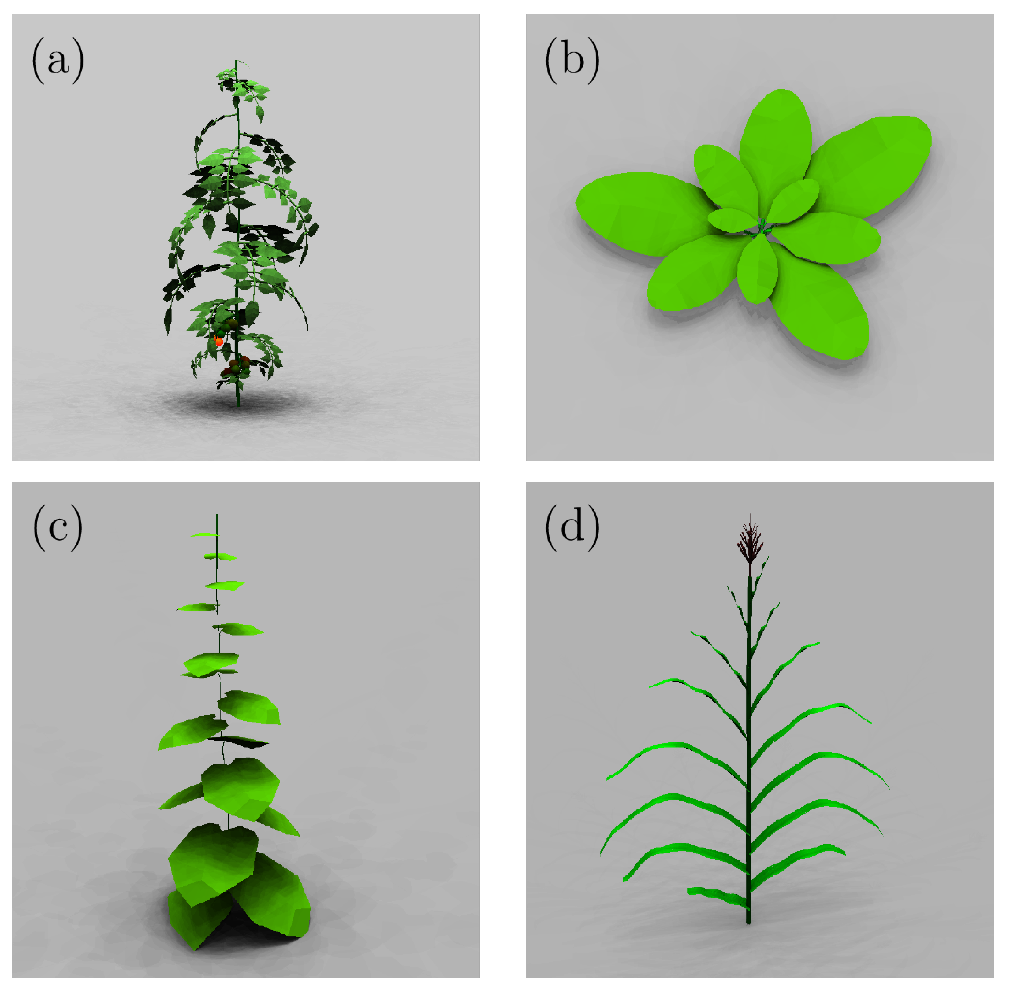
Figure 1. Screenshots of rendered images of the four plant shoot models used within this study including (a) tomato, (b) arabidopsis, (c) greenhouse cucumber, and (d) maize.
Remotesensing 14 04727 g001
Figure 2. Screenshots of the 3D tomato plant model as described in Zhang et al. [35]. (a) a rendered image of the whole virtual plant (uniformly coloured), (b) a detail enlargement of leaf with rank 13 with the underlying wireframe triangulation, and (c) an image of a single leaflet with the overlay of the wireframe triangulation. A leaflet is modelled of eight vertical mirror symmetric arranged faces (triangles), making it in total 16 faces for one single leaflet. The whole plant consists roughly of 25.7 k vertices forming a triangulation of about 8.5 k faces.
Remotesensing 14 04727 g002
Figure 3. Top- (a) and side-view (b) of the virtual scanner hemisphere with the synthetic 3D tomato plant model in the centre of the scene. Blue spheres indicate the position of spatial points from where the 3D scanning is performed. The scanning sphere consists of 13 layers with 25 measuring points on each layer, resulting in 325 measuring points used for each scan. The thin yellow lines—length set to 30 centimetres for visualization only—represent a small fraction of the rays used for the scanning.
Remotesensing 14 04727 g003
Figure 4. Top-view visualization of the tomato plant model for the three thinning scenarios: (a) the original complete plant, (b) random thinning, (c) inside to outside thinning, and (d) outside to inside thinning, all at 30 % .
Remotesensing 14 04727 g004
Figure 5. Visualization of the scanned point cloud (green dots) of the complete (initial) plant and the convex hull drawn as transparent blue for all four plant species used in this study: (a) tomato, (b) arabidopsis, (c) greenhouse cucumber, and (d) maize.
Remotesensing 14 04727 g005
Figure 6. Visualization of the hit density (ray hits/mm 2 ) on the example of the full tomato model at zero perturbation in (a) top-, and (b) side-view, as well the the normalized histogram in sub-figure (c). Each triangle of the mesh model is coloured according to the number of rays that had hit is and the resulting hit density.
Remotesensing 14 04727 g006
Figure 7. Visualization of the surrounding half ellipsoid (a), that is used to estimate the relation between triangle area and number of hits. As shown in (b) the hit density per square millimeter triangle area [hit/mm 2 ] is quite homogenise around the surface of the ellipsoid with a slight higher concentration on the north pole and a bit lower at the south pole as expected from the used geometry from the hemispherical shape of the scanner dome. The chart in (c) shows the relation between the number of hits per triangle versus the area of it.
Remotesensing 14 04727 g007
Figure 8. Statistics of hit density of half-ellipsoid triangles. Visualization of the median and mean hit density along 10 area classes from zero to a maximum of 250 mm 2 and a bin width of 25 mm 2 . The low variance between the individual mean and median values to the overall values proves that there is—as expected—a constant relation relation between the size of the triangles and the observed hit density. The hit density of a “fully visible” triangle is ρ m = 0.0959 hits/mm 2 .
Remotesensing 14 04727 g008
Figure 9. Summary of the simulated dependency of normalized phenotypic traits on the percentage of plant area loss for four different plant models and three different area perturbation scenarios including random (red), outside-to-inside (blue), and inside-to-outside (green) perturbation scenarios. The last row shows the dependency of the normalized visible plant area on the percentage of the total area loss for four plant models and the three alternative perturbation scenarios.
Remotesensing 14 04727 g009
Figure 10. Visualization of the relative visible area for each perturbation scenario in different plant types.
Remotesensing 14 04727 g010
Figure 11. Visualization of the same phenotypic features as in Figure 9 but in dependency on the relative visible plant area shown in the last row of Figure 9.
Remotesensing 14 04727 g011
Figure 12. Example of analysis and visualization of smoothness of tomato point clouds (PC). (a) Histograms of smoothness factor (SF) from Equation (1)) of original and randomly perturbed tomato point clouds. The arrow in the histogram plot indicates the elevation of amount of corner/edge points with a larger smoothness factor (SF) in the randomly perturbed model. (b) Visualization of original vs. randomly perturbed full and boundary point clouds of the tomato plant. Boundary points were detected using the smoothness factor values larger than 0.5. The colour map indicates the SF values ranging in [ 0 , 1 ] .
Remotesensing 14 04727 g012
Figure 13. Exemplary comparison of point cloud smoothness of different plants (A—arabidopsis, C—cucumber, M—maize, T—tomato) in dependency on random model perturbation. (a) Average smoothness factor (SF) of different plants, (b) stdev of SF distribution in different plants, (c) fraction of boundary points in % detected by thresholding of SF values larger than >0.5, and (d) t-test values computed from comparison of SF distributions of randomly perturbed plant point clouds vs. original (unperturbed) models.
Remotesensing 14 04727 g013
Table 1. Summary of the plant model properties. Starting from the number of geometric primitive objects of the original 3D model, i.e., number of leaves and internodes and morphological traits like plant dimensions, to the number of vertices and faces of the triangulated mesh.
PlantNumberNumber ofMaxMaxNumberNumberMean Face
Modelof LeavesInternodesHeight [m]Radius [m]of Verticesof FacesArea [mm 2 ]
Tomato21211.70.4325,6748558142.53
Arabidopsis10110.030.0636001200189.92
Maize14152.50.9715,4505150699.83
Cucumber17182.00.435793193112.74
Table 2. Overview of the faces (F) and areas (A) that are “visible” to laser scanner in original (unperturbed) plant models as relative ratios to their known full-plant values, i.e., F v i s / F a l l re. A v i s / A a l l .
SpeciesVisible Faces [%]Visible Area [%]
Tomato0.590.78
Arabidopsis0.790.81
Maize0.670.94
Cucumber0.480.94
Table 3. Summary of the linear correlation between the phenotypic features from Figure 11 and the visible plant area for all three geometry perturbation scenarios (random, inside-to-outside (i2o), and outside-to-inside (o2i)) in the range of 0–30% including correlation coefficients ( ρ ) and corresponding p-values. N a N entries indicate a uncorrelated relationship between a feature and the visible plant area.
HeightPCA1PCA2VolumeAbsorptionArea
ρ , p-Value ρ , p-Value ρ , p-Value ρ , p-Value ρ , p-Value ρ , p-Value
Tomato
RandomNaN, NaN−0.75, 8.11 × 10 4 0.87, 1.10 × 10 5 0.94, 5.88 × 10 8 1.00, 4.75 × 10 19 NaN, NaN
i2oNaN, NaN0.98, 1.26 × 10 11 0.95, 2.57 × 10 8 0.78, 3.46 × 10 4 0.99, 1.90 × 10 13 1.00, 2.00 × 10 103
o2iNaN, NaN0.98, 6.60 × 10 12 0.98, 6.00 × 10 12 1.00, 4.57 × 10 18 1.00, 3.26 × 10 20 1.00, 9.13 × 10 107
Maize
RandomNaN, NaN0.80, 1.69 × 10 4 0.87, 1.15 × 10 5 0.94, 9.83 × 10 8 1.00, 3.03 × 10 25 1.00, 4.98 × 10 102
i2oNaN, NaN0.95, 1.93 × 10 8 0.87, 1.28 × 10 5 0.97, 5.40 × 10 10 0.99, 7.83 × 10 14 1.00, 9.13 × 10 107
o2iNaN, NaN0.99, 3.19 × 10 13 0.92, 3.67 × 10 7 1.00, 1.34 × 10 23 1.00, 1.12 × 10 20 1.00, 0.00
Cucumber
RandomNaN, NaN−0.85, 3.44 × 10 5 −0.73, 1.34 × 10 3 0.91, 8.62 × 10 7 1.00, 4.25 × 10 21 NaN, NaN
i2oNaN, NaN0.43, 9.76 × 10 2 0.42, 1.02 × 10 1 0.75, 7.96 × 10 4 0.98, 1.49 × 10 11 1.00, 4.36 × 10 106
o2iNaN, NaN0.99, 1.18 × 10 13 1.00, 4.57 × 10 16 1.00, 1.97 × 10 21 1.00, 2.20 × 10 20 1.00, 0.00
Arabidopsis
Random0.71, 1.91 × 10 3 0.89, 3.51 × 10 6 0.83, 5.80 × 10 5 −0.77, 5.00 × 10 4 1.00, 2.70 × 10 22 1.00, 0.00
i2oNaN, NaN−0.88, 5.59 × 10 6 0.87, 9.27 × 10 6 0.73, 1.44 × 10 3 0.95, 1.74 × 10 8 1.00, 7.14 × 10 109
o2i0.82, 1.07 × 10 4 0.98, 6.08 × 10 12 0.99, 1.04 × 10 14 1.00, 1.18 × 10 21 1.00, 3.57 × 10 23 1.00, 0.00
Publisher’s Note: MDPI stays neutral with regard to jurisdictional claims in published maps and institutional affiliations.