Joint Inversion of 3D Gravity and Magnetic Data under Undulating Terrain Based on Combined Hexahedral Grid

Abstract

As an effective underground imaging method, the joint inversion of the gravity and magnetic data has an important application in the comprehensive interpretation of mineral exploration, and unstructured modeling is the key to accurately solving its topographic problem. However, the traditional tetrahedral grid can only impose the gradient-based constraints approximately, owing to its poor arrangement regularity. To address the difficulty of applying a cross-gradient constraint in an unstructured grid, we propose a joint inversion based on a combined hexahedral grid, which regularly divides the shallow part into curved hexahedrons and the deep part into regular hexahedrons. Instead of a cross-gradient in the spatial sense, we construct a geometric sense “cross-gradient” for a structural constraint to reduce the influence of approximation. In addition, we further correct the traditional sensitivity-based weighting function according to element volume, to make it suitable for an unstructured grid. Model tests indicate that the new grid can impose the cross-gradient constraint more strongly, and the proposed correction can effectively solve the false anomaly caused by the element volume difference. Finally, we apply our method to the measured data from a mining area in Huzhong, Heilongjiang Province, China, and successfully invert out the specific location of a known skarn deposit, which further proves its practicability.

1. Introduction

With the characteristics of fast measurement, wide coverage, and dense sampling, the gravity and magnetic data are widely used in mineral prospecting, geological mapping, and basin study and have significant value in remote sensing imagery. However, whether from satellites, airplanes, or the Earth’s surface, measurements are easily affected by topographic relief, which will influence the reliability of interpretation. The classical approach to solving this problem has been to remove the terrain effect from observations by a forward operator, thus computing the Bouguer anomaly and performing inversion with a flat terrain model, but the sources between the terrain and the plane may not be reflected accurately. In recent years, methods simulating the terrain with an unstructured grid have attracted more geophysicists. Various gravity and magnetic forward methods for unstructured grids have been proposed, such as the analytical expression, finite-element, and finite-difference methods [1,2,3], and a method combining a structured grid with an unstructured grid has been presented to improve the computational efficiency [4].

A single type of geophysical data can only evaluate the underground from a single point of view, while using multiple pieces of data to study it from multiple perspectives—for example, joint inversion—is conducive to predicting information more comprehensively and accurately. Joint inversion can be divided into two categories according to the construction of the joint relationship. One is the joint inversion that converts physical parameters through empirical relations [5,6,7], and the other is the joint inversion that constrains the structural similarity. As an example of the latter, the cross-gradient method searches for models with similar structure by constraining the gradient direction of different physical parameters to be consistent, and it is widely used because it does not rely on empirical relations or initial model assumptions [8,9,10,11,12]. Particularly in the comprehensive interpretation of the gravity and magnetic data, the cross-gradient joint inversion has achieved many successful application results [13,14,15,16,17,18].

Until now, the research on joint inversion has focused mostly on the flat terrain model composed of regular hexahedrons and less on the undulating terrain model with an unstructured grid. Ozyildirim et al. studied the two-dimensional joint inversion of direct-current resistivity and radio-magnetotelluric data based on a triangular grid, which is realized by directly consolidating the data sets because the two methods correspond to the same physical property [19]. Lelievre et al. proposed a joint inversion of seismic travel times and gravity data based on a tetrahedral grid, which uses multiple coupling measures including empirical relations, physical property distribution information, and cross-gradient constraints [20]. Jordi et al. applied a tetrahedral grid to the joint inversion of three-dimensional resistivity and ground-penetrating radar data and realized the cross-gradient constraint from the physical scale rather than the grid element scale [21]. Yin et al. proposed a structural constraint method based on the Pearson correlation from the perspective of statistics and pointed out that the method can be applied to joint inversion under an unstructured grid [22].

The existing joint inversions based on an unstructured grid mainly use tetrahedrons or triangles to divide the model. However, it is not easy to calculate physical gradients for this kind of grid because of its irregular element connection. A useful method proposed by Lelievre and Farquharson is to calculate the derivatives in adjacent element directions first and combine them linearly to obtain the derivatives in the X, Y, and Z directions [23]. Nonetheless, this process is relatively complex, and its result is approximate. As a result, the application of a cross-gradient constraint for an unstructured grid is limited, owing to its dependence on gradient calculation. In addition, although the sensitivity-based weighting function [24,25], which is commonly used for the depth weighting of the gravity and magnetic inversion, has achieved good results in regular models, it cannot be directly used for an unstructured grid. The element volume difference makes it easier for anomalies to gather on small elements, which may result in a false anomaly problem.

In this paper, we propose a cross-gradient joint inversion of the gravity and magnetic data based on a combined hexahedral grid. The grid uses curved hexahedrons to simulate terrain in the shallow part of the model, with forward modeling that can be realized by isoparametric transformation and Gaussian integration [26], and regular hexahedrons forwarded by analytical expression to divide the deep part for efficiency. Due to its regular element arrangement, we can replace the traditional cross-gradient in the spatial sense with a geometric sense “cross-gradient” for the adjacent elements to constrain the structural similarity, making it easier to apply to models with terrain and better avoid the influence of approximation in gradient calculation. Moreover, we further correct the traditional sensitivity-based weighting function according to element volume, which we named “element volume correction”, to make it suitable for an unstructured grid and solve the false anomaly problem. We verify the effectiveness of our algorithm through three groups of theoretical model tests and finally apply it to the measured data from a skarn mining area in Huzhong, Heilongjiang Province, China, proving its practicability.

2. Methods

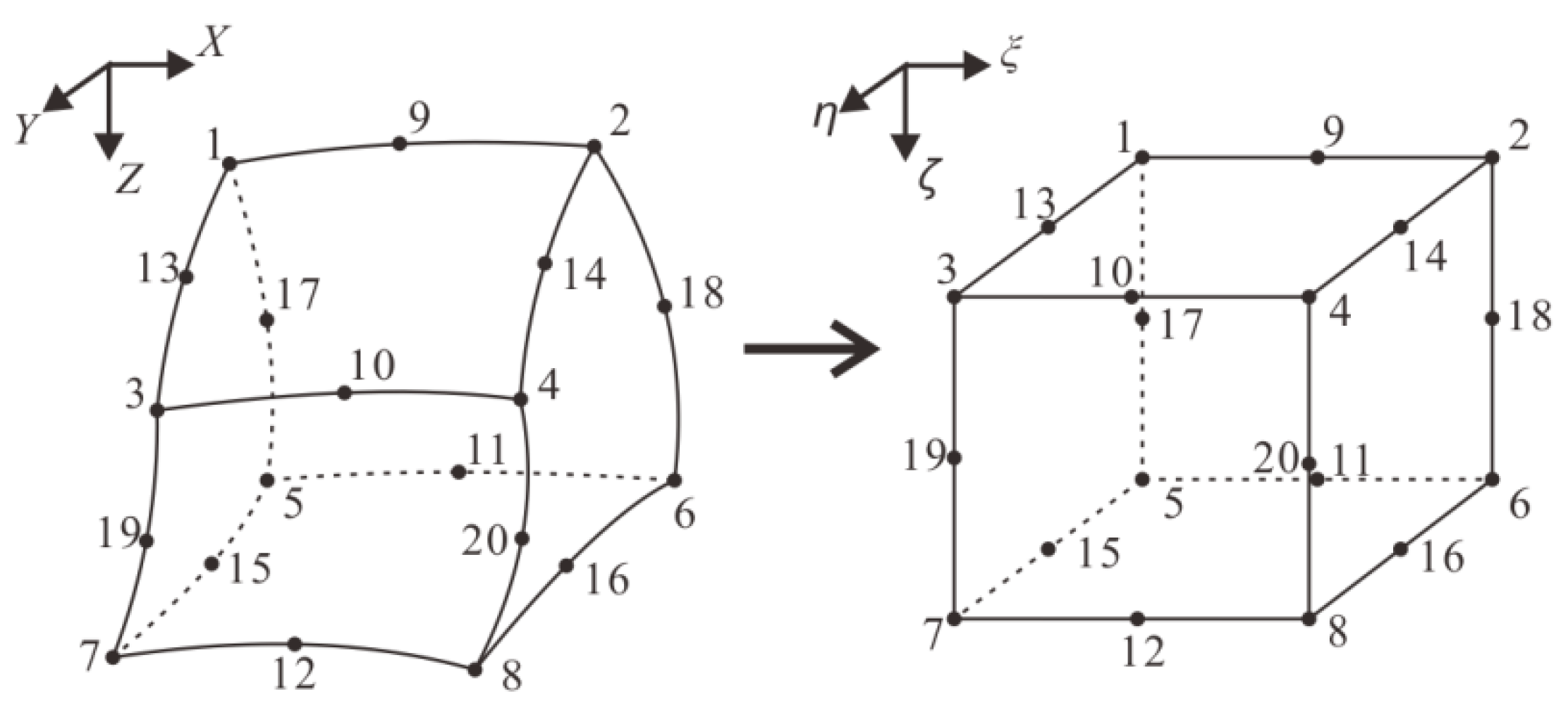
2.1. Curved Hexahedron Forward Theory

Forward modeling is the basis of inversion. For regular hexahedrons, it is easy to calculate their response by analytical expressions [27,28]. In this section, we mainly focus on the forward theory of curved hexahedrons. The well-known gravity (V_z) and magnetic (ΔT) forward integral formulas of a three-dimensional body in a conventional physical domain are as follows:

$$V_z=G\rho {\displaystyle \underset{v}{\iiint }\frac{(z_0-z)}{{({(x_0-x)}^2+{(y_0-y)}^2+{(z_0-z)}^2)}^{3/2}}}\mathrm{d}x\mathrm{d}y\mathrm{d}z,$$

(1)

$$\begin{array}{ll}{B}_x =\frac{{\mu }_{0}M}{4\mathsf{\pi }}& [\cos {\alpha }_s{\displaystyle \underset{v}{\iiint }\frac{2{(x_0-x)}^2-{(y_0-y)}^2-{(z_0-z)}^2}{{({(x_0 -x)}^2 +{(y_0 -y)}^2 +{(z_0 -z)}^2)}^{5/2}}}\mathrm{d}x \mathrm{d}y \mathrm{d}z +\\ & 3\cos {\beta }_s{\displaystyle \underset{v}{\iiint }\frac{(x_0-x)(y_0-y)}{{({(x_0 -x)}^2 +{(y_0 -y)}^2 +{(z_0 -z)}^2)}^{5/2}}}\mathrm{d}x \mathrm{d}y \mathrm{d}z +\\ & 3\cos {\gamma }_s{\displaystyle \underset{v}{\iiint }\frac{(x_0-x)(z_0-z)}{{({(x_0 -x)}^2 +{(y_0 -y)}^2 +{(z_0 -z)}^2)}^{5/2}}}\mathrm{d}x \mathrm{d}y \mathrm{d}z],\end{array}$$

(2)

$$\begin{array}{ll}{B}_y =\frac{{\mu }_{0}M}{4\mathsf{\pi }}& [3\cos {\alpha }_s{\displaystyle \underset{v}{\iiint }\frac{(x_0-x)(y_0-y)}{{({(x_0 -x)}^2 +{(y_0 -y)}^2 +{(z_0 -z)}^2)}^{5/2}}}\mathrm{d}x \mathrm{d}y \mathrm{d}z +\\ & \cos {\beta }_s{\displaystyle \underset{v}{\iiint }\frac{2{(y_0-y)}^2-{(x_0-x)}^2-{(z_0-z)}^2}{{({(x_0 -x)}^2 +{(y_0 -y)}^2 +{(z_0 -z)}^2)}^{5/2}}}\mathrm{d}x \mathrm{d}y \mathrm{d}z +\\ & 3\cos {\gamma }_s{\displaystyle \underset{v}{\iiint }\frac{(y_0-y)(z_0-z)}{{({(x_0 -x)}^2 +{(y_0 -y)}^2 +{(z_0 -z)}^2)}^{5/2}}}\mathrm{d}x \mathrm{d}y \mathrm{d}z],\end{array}$$

(3)

$$\begin{array}{ll}{B}_z =\frac{{\mu }_{0}M}{4\mathsf{\pi }}& [3\cos {\alpha }_s{\displaystyle \underset{v}{\iiint }\frac{(x_0-x)(z_0-z)}{{({(x_0 -x)}^2 +{(y_0 -y)}^2 +{(z_0 -z)}^2)}^{5/2}}}\mathrm{d}x \mathrm{d}y \mathrm{d}z +\\ & 3\cos {\beta }_s{\displaystyle \underset{v}{\iiint }\frac{(y_0-y)(z_0-z)}{{({(x_0 -x)}^2 +{(y_0 -y)}^2 +{(z_0 -z)}^2)}^{5/2}}}\mathrm{d}x \mathrm{d}y \mathrm{d}z +\\ & \cos {\gamma }_s{\displaystyle \underset{v}{\iiint }\frac{2{(z_0-z)}^2-{(x_0-x)}^2-{(y_0-y)}^2}{{({(x_0 -x)}^2 +{(y_0 -y)}^2 +{(z_0 -z)}^2)}^{5/2}}}\mathrm{d}x \mathrm{d}y \mathrm{d}z],\end{array}$$

(4)

$$\Delta T=B_x\cos {\alpha }_t+ B_y\cos {\beta }_t+ B_z\cos {\gamma }_t,$$

(5)

where (x₀, y₀, z₀) is the coordinate of the observation point, (x, y, z) is the coordinate of the abnormal body with volume of v and density of ρ, G is the gravitational constant, and μ₀ is the magnetic permeability in a vacuum. cosα_s, cosβ_s, and cosγ_s are the directional cosines of magnetization vector M, and cosα_t, cosβ_t, and cosγ_t are the directional cosines of the normal magnetic field. In this paper, we assume the magnetization direction is consistent with the normal field.

For curved hexahedrons, Equations (1)–(5) have a rather complex integration region, which is difficult to realize by numerical simulation directly. Based on the isoparametric transformation theory in the finite-element method, a 20-node curved hexahedron with a quadratic-function-based surface in the physical domain (x, y, z) can be transformed into a regular one in the computational domain (ξ, η, ζ) (Figure 1). The coordinates of nodes after transformation are shown in

Table 1. Node coordinates in the computational domain.

i	1	2	3	4	5	6	7	8	9	10	11	12	13	14	15	16	17	18	19	20
ξi	−1	1	−1	1	−1	1	−1	1	0	0	0	0	−1	1	−1	1	−1	1	−1	1
ηi	−1	−1	1	1	−1	−1	1	1	−1	1	−1	1	0	0	0	0	−1	−1	1	1
ζi	−1	−1	−1	−1	1	1	1	1	−1	−1	1	1	−1	−1	1	1	0	0	0	0

, and the conversion relationships are as follows:

$$x={\displaystyle \sum _{i=1}^{20}{N}_i{x}_i}, y={\displaystyle \sum _{i=1}^{20}{N}_i{y}_i}, z={\displaystyle \sum _{i=1}^{20}{N}_i{z}_i},$$

(6)

$$N_i\left(\xi ,\eta ,\zeta \right)=\{\begin{array}{ll}\frac{1}{8}\left(1+{\xi }_i\xi \right)\left(1+{\eta }_i\eta \right)\left(1+{\zeta }_i\zeta \right)\left({\xi }_i\xi +{\eta }_i\eta + {\zeta }_i\zeta - 2\right)& i=1\sim 8\hspace{0.17em} \hspace{1em}\hspace{0.17em}\\ \frac{1}{4}\left(1 - {\xi }^2\right)\left(1 + {\eta }_i\eta \right)\left(1 + {\zeta }_i\zeta \right)& i=9\sim 12 \hspace{0.17em} \hspace{0.17em}\\ \frac{1}{4}\left(1 + {\xi }_i\xi \right)\left(1 - {\eta }^2\right)\left(1 + {\zeta }_i\zeta \right)& i=13\sim 16 \\ \frac{1}{4}\left(1 + {\xi }_i\xi \right)\left(1 + {\eta }_i\eta \right)\left(1 - {\zeta }^2\right)& i=17\sim 20\end{array}.$$

(7)

Replacing x, y, z with ξ, η, ζ by Equations (6) and (7), the original integral formula in the physical domain becomes the following computational domain form:

$${\displaystyle \underset{v}{\iiint }f(x,y,z)} \mathrm{d}x \mathrm{d}y \mathrm{dz} ={\displaystyle {\int }_{-1}^1{\displaystyle {\int }_{-1}^1{\displaystyle {\int }_{-1}^{1}f \left[x\left(\xi ,\eta ,\zeta \right),y\left(\xi ,\eta ,\zeta \right),z\left(\xi ,\eta ,\zeta \right)\right]}}} \omega \left(\xi ,\eta ,\zeta \right) \mathrm{d}\xi \mathrm{d}\eta \mathrm{d}\zeta ,$$

(8)

$$\omega \left(\xi ,\eta ,\zeta \right) =\left|\begin{array}{ccc}\frac{\partial x}{\partial \xi }& \hspace{1em}\frac{\partial y}{\partial \xi }& \hspace{1em}\frac{\partial z}{\partial \xi }\\ \frac{\partial x}{\partial \eta }& \hspace{1em}\frac{\partial y}{\partial \eta }& \hspace{1em}\frac{\partial z}{\partial \eta }\\ \frac{\partial x}{\partial \zeta }& \hspace{1em}\frac{\partial y}{\partial \zeta }& \hspace{1em}\frac{\partial z}{\partial \zeta }\end{array}\right|,$$

(9)

where f is applicable to the integral kernel in Equations (1)–(5). The right end term of Equation (8) with a regular integration region can be simulated by the Gaussian integral method. Then, the forward modeling of the curved hexahedron can be realized, and Kim et al. proved its reliability [26]. It is worth noting that the accuracy of the Gauss integral is easily affected by near singularity. In this connection, when an observation point is too close to an element, we subdivide the element and use more Gaussian nodes to calculate integral. The values of each subelement are accumulated as the forward response of the target element. This treatment can effectively weaken the influence of near singularity but will also increase the computational burden to a certain extent.

2.2. Cross-Gradient Joint Inversion Method

In this paper, we adopt the strategy of alternately iterating two physical properties for joint inversion, with objective functions that are constructed as follows:

$$\phi \left(m_{\rho }\right)={\phi }_d\left(m_{\rho }\right)+{\lambda }_{m\rho }{\phi }_m\left(m_{\rho }\right)+{\lambda }_{j\rho }{\phi }_j\left(m_{\rho },m_{\kappa }\right),$$

(10)

$$\phi \left(m_{\kappa }\right)={\phi }_d\left(m_{\kappa }\right)+{\lambda }_{m\kappa }{\phi }_m\left(m_{\kappa }\right)+{\lambda }_{j\kappa }{\phi }_j\left(m_{\rho },m_{\kappa }\right),$$

(11)

$${\phi }_j\left(m_{\rho },m_{\kappa }\right)=t^{\mathrm{T}} \left(m_{\rho },m_{\kappa }\right) \hspace{0.17em}t\left(m_{\rho },m_{\kappa }\right),$$

(12)

where m_ρ and m_κ represent density and magnetization; φ_d, φ_m, and φ_j correspond to the constraint terms of data, model, and cross-gradient, respectively; and λ is their weight coefficient. The cross-gradient function t in Equation (12) was defined by Gallardo and Meju [8] as:

$$t\left(x , y ,\hspace{0.17em}z\right)=\nabla m_{\rho }\left(x , y ,\hspace{0.17em}z\right)\times \nabla m_{\kappa }\left(x , y ,\hspace{0.17em}z\right) ,$$

(13)

with components in three directions that are:

$$t_x=\frac{\partial m_{\rho }}{\partial y}\frac{\partial m_{\kappa }}{\partial z}-\frac{\partial m_{\rho }}{\partial z}\frac{\partial m_{\kappa }}{\partial y},$$

(14)

$$t_y=\frac{\partial m_{\rho }}{\partial z}\frac{\partial m_{\kappa }}{\partial x}-\frac{\partial m_{\rho }}{\partial x}\frac{\partial m_{\kappa }}{\partial z},$$

(15)

$$t_z=\frac{\partial m_{\rho }}{\partial x}\frac{\partial m_{\kappa }}{\partial y}-\frac{\partial m_{\rho }}{\partial y}\frac{\partial m_{\kappa }}{\partial x}.$$

(16)

By minimizing Equations (10) and (11), we can obtain the iterative expressions of the inversion models:

$$m_{\rho }^{{}_{k+1}}-m_{\rho }^{{}_k}={\left(J_{\rho }^{\mathrm{T}}{C}_{d\rho }^{-1}{J}_{\rho }+{\lambda }_{ m\rho }{C}_{m \rho }^{-1}+{\lambda }_{j\rho }{B}_{\rho }^{\mathrm{T}}{B}_{\rho }\right)}^{-1}\left[J_{\rho }^{\mathrm{T}}{C}_{d\rho }^{-1}\left(d_{\rho }-F_{\rho }\left(m_{\rho }\right)\right)-{\lambda }_{j\rho }{B}_{\rho }^{\mathrm{T}}t\right],$$

(17)

$$m_{\kappa }^{{}_{k+1}}-m_{\kappa }^{{}_k}={\left(J_{\kappa }^{\mathrm{T}}{C}_{d \kappa }^{-1}{J}_{\kappa }+{\lambda }_{ m\kappa }{C}_{m \kappa }^{-1}+{\lambda }_{j\kappa }{B}_{\kappa }^{\mathrm{T}}{B}_{\kappa }\right)}^{-1}\left[J_{\kappa }^{\mathrm{T}}{C}_{d \kappa }^{-1}\left(d_{\kappa }-F_{\kappa }\left(m_{\kappa }\right)\right)-{\lambda }_{j\kappa }{B}_{\kappa }^{\mathrm{T}}t\right],$$

(18)

where k is the iteration number; J is the sensitivity matrix; C_d⁻¹ and C_m⁻¹ are the covariance matrices of data and model, respectively; B is the derivative of t, d is the observation data; and F is the forward operator. To obtain results with a clearer boundary and more obvious amplitude, we adopt a focus constraint for Equations (17) and (18) [29,30,31]:

$$C_m^{-1}=R_e^{\mathrm{T}}{R}_s^{\mathrm{T}}{R}_s{R}_e,$$

(19)

$$R_e=diag\left(1/\sqrt{ \left[{\left(m-m_{ref}\right)}^2+e^2\right]}\right),$$

(20)

where R_e is the focus matrix, R_s is the sensitivity-based weighting matrix, and m_ref is the reference model. If there is no reference model, we set m_ref to 0. The constant e represents the focusing factor, and a smaller e usually makes the anomaly easier to focus.

$${\lambda }_j^k={\Lambda }_{j0}\frac{{\phi }_d^k}{{\phi }_j^k},$$

(21)

$${\lambda }_m^0={\Lambda }_{m0}\frac{{\Vert \mathrm{diag}\left(J^{\mathrm{T}}{C}_d^{-1}J\right)\Vert }_1}{{\Vert \mathrm{diag}\left(C_{m }^{-1}\right)\Vert }_1}.$$

(22)

In addition, we assign λ_j for Equations (17) and (18) as Equation (21) to make it more controllable, where Λ is a fixed constant. Since the φ_m before the first iteration is usually 0, we use another kind of ratio as Equation (22) to assign the initial λ_m, which will be gradually reduced by multiplying a constant in subsequent iterations where diag means the main diagonal of the matrix. Generally, we try multiple groups of λ with a fixed number of iterations and select the optimal one according to data fitting, model recovery, and cross-gradient decline.

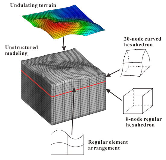
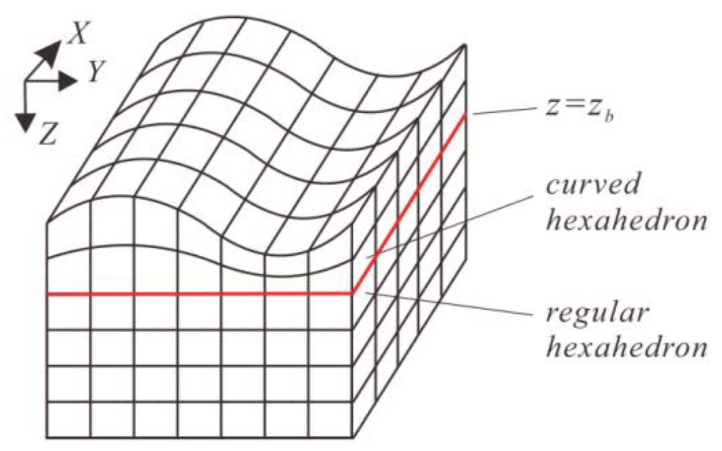
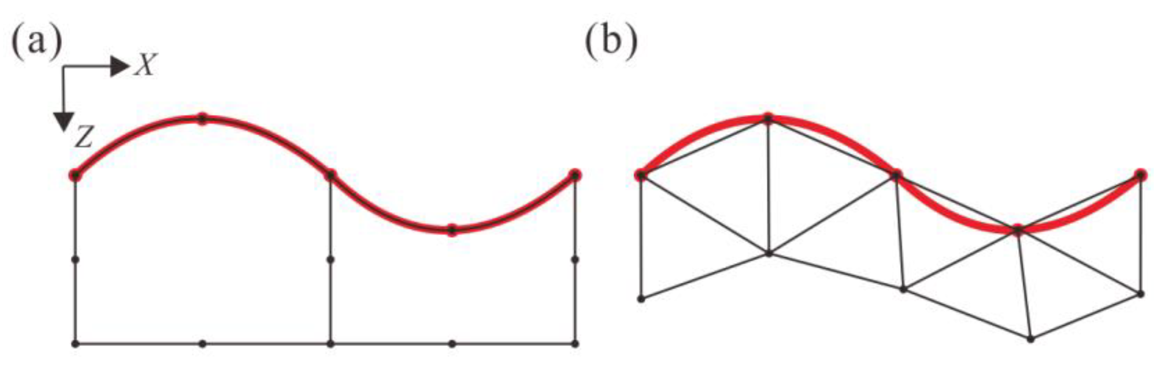
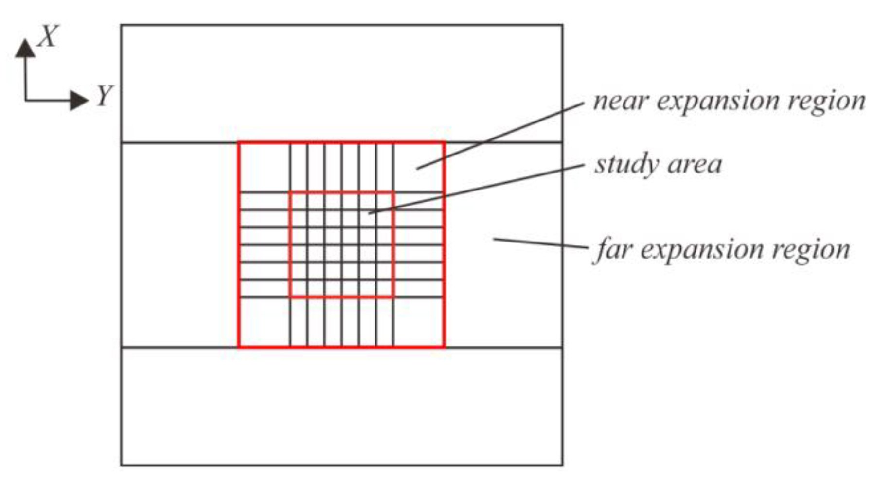
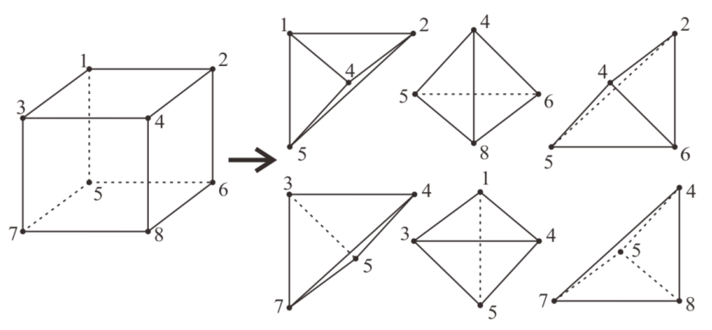
2.3. Combined Hexahedral Grid

Equations (14)–(16) require the physical gradients in the X, Y, and Z directions. For the tetrahedral grid, the common method is to calculate the gradient g_0,j from a central element m₀ to its adjacent four m_j as Equation (23) first and combine them in some way to obtain the target gradient g₀ as Equation (24) [23]:

$$g_{0,j}=\frac{m_j-m_0}{d_{0,j}}u{ }_{0,j}\hspace{1em},j=1~4,$$

(23)

$$g_0={\displaystyle \sum _{j=1}^4{l}_j} g_{0,j}.$$

(24)

where d is the distance between element centroids, u is the unit vector, and l represents the weight of the vector combination. However, this result is approximate, which makes the cross-gradient constraint difficult to apply to models with terrain. In this connection, we designed a combined hexahedral grid for the cross-gradient joint inversion.

As shown in Figure 2, the shallow part of the model (z ≤ z_b) is divided into curved hexahedrons with equal spacing in the X and Y directions and equal number in the Z direction, called the “irregular layer”, and the layer thickness at the same (x, y) is uniform. The deep part of the model (z > z_b) is divided into regular hexahedrons with equal spacing, which is called the “regular layer”. The interface z_b can be set to a flexible position below the lowest terrain, and the division number of irregular layers should make the elements below the highest terrain meet the desired resolution. Considering that it is not easy to make a clear judgment on the bending direction of deep grids in advance, and the resolution of the gravity and magnetic data is not high enough to distinguish the edge details of an element-sized body, this combined grid has almost the same resolution as one that uses only curved hexahedrons. However, it ensures a higher efficiency because the forward speed of the regular hexahedron with the analytical formula is much higher than that of the curved hexahedron with the Gaussian integral.

Although the above grid no longer needs to synthesize gradients from four different directions like a tetrahedral grid and has a more regular arrangement, the position relationships between elements in the irregular layers are not orthogonal (Figure 2). Therefore, the grid still cannot construct a cross-gradient directly by the same method as a regular grid. Considering that the discrete cross-gradient finally constrains the physical relationships between elements, and the gradients are only calculated as transitions, we can directly construct the constraints on the elements. Since a hexahedral element and its adjacent three in the positive directions of X, Y, and Z are independent of each other, the relationships between their physical changes can be considered as orthogonal from a geometric view. With this connection, we can directly calculate the differences between the physical properties of current element m_c and its adjacent three (m_r, m_f, and m_d) as geometric sense “gradients” and use them to replace the spatial sense gradients in Equations (14)–(16). Then, Equations (14)–(16) can be discretized into the following forward-difference form, which is quite similar to that of a regular grid [13]:

$$t_x=\frac{4}{\Delta y\Delta z}\left[m_{\rho f}\left(m_{\kappa d}-m_{\kappa c}\right)-m_{\rho c}\left(m_{\kappa d}-m_{\kappa f}\right)-m_{\rho d}\left(m_{\kappa f}-m_{\kappa c}\right)\right],$$

(25)

$$t_y=\frac{4}{\Delta x\Delta z}\left[m_{\rho d}\left(m_{\kappa r}-m_{\kappa c}\right)-m_{\rho c}\left(m_{\kappa r}-m_{\kappa d}\right)-m_{\rho r}\left(m_{\kappa d}-m_{\kappa c}\right)\right],$$

(26)

$$t_z=\frac{4}{\Delta y\Delta x}\left[m_{\rho r}\left(m_{\kappa f}-m_{\kappa c}\right)-m_{\rho c}\left(m_{\kappa f}-m_{\kappa r}\right)-m_{\rho f}\left(m_{\kappa r}-m_{\kappa c}\right)\right],$$

(27)

where Δx, Δy, and Δz are the distances between the element centroids. This result is no longer the cross-gradient for the X, Y, and Z directions in a spatial sense, but a geometric sense “cross-gradient” for the adjacent elements, which is essentially consistent with the thrust of the former, that is, the structural similarity constraint.

For irregular layers, there are still some approximations in obtaining Δx, Δy, and Δz. Thus, we take t_x as an example to analyze the error modes of the cross-gradient calculation under these two grids. For the tetrahedral grid, supposing there are some errors ε in synthesizing the X, Y, and Z gradients, Equation (14) will take the following form:

$$t_x=\left(\frac{\partial m_{\rho }}{\partial y}+{\epsilon }_1\right)\left(\frac{\partial m_{\kappa }}{\partial z}+{\epsilon }_2\right)-\left(\frac{\partial m_{\rho }}{\partial z}+{\epsilon }_3\right)\left(\frac{\partial m_{\kappa }}{\partial y}+{\epsilon }_4\right).$$

(28)

It can be seen from Equation (28) that these errors are coupled with physical values in a complex form, owing to the direction deflection involved in gradient synthesis, which may influence the decline of the cross-gradient. In contrast, our hexahedral grid avoids that deflection, and the error only exists in Δx, Δy, and Δz:

$$t_x=\frac{4}{\left(\Delta y + {\epsilon }_1\right)\left(\Delta z + {\epsilon }_2\right)}\left[m_{\rho f}\left(m_{\kappa d}-m_{\kappa c}\right)-m_{\rho c}\left(m_{\kappa d}-m_{\kappa f}\right)-m_{\rho d}\left(m_{\kappa f}-m_{\kappa c}\right)\right].$$

(29)

The error term in Equation (29) does not intervene in the coupling of physical elements and will hardly affect the approach of t_x to 0. In this way, the method using the geometric sense “cross-gradient” in the combined hexahedral grid can better reduce the influence of approximation and make the structural constraint easier to implement.

It is worth mentioning that the curved hexahedron also has an advantage in terrain simulation. Taking Figure 3 as an example, the red part represents the continuous terrain and its discrete sampling, while the black part represents the geometric elements used to simulate the terrain and its nodes. Compared with the tetrahedron (Figure 3b), the hexahedron with the quadratic-function-based surface (Figure 3a) can simulate the same terrain with fewer elements. For divisions with a similar element number, the simulation accuracy of the curved hexahedron is usually higher than that of the tetrahedron because it has many more geometric nodes in an element, although this usually requires a more intensive terrain sampling.

Since the physical difference between the two sides of undulating terrain cannot be ignored, we used a real physical property instead of a residual to assign value to the elements and expand the model horizontally to eliminate the influence of the edge effect. As shown in Figure 4, the expansion zone consists of two parts: the near region and the far region, which are constructed by regular hexahedrons with background physical properties [32]. For a hexahedron in the near region, the elevation of its upper surface can be made consistent with its nearest elevation-known node, if there is no exact information. For hexahedrons in the far region, we set their elevations as the average value of the study area. The range of the near region can be several times the study area, while the far region can be extended to infinity. The expansion zone does not participate in model iteration, so its response should be subtracted from the observation data before inversion.

2.4. Element Volume Correction

To solve the skin effect in the gravity and magnetic inversion, a sensitivity-based weighting function, as shown in Equation (30), was proposed as the R_s in Equation (19) [24,25]. The matrix can well capture the decay related to integral sensitivity on the main diagonal of J^TC_d⁻¹J, which is the main part of the left end term in Equations (17) and (18), and make up for its influence, that is, the solution Δm tends to appear in elements with high sensitivity.

$$R_s\left(j , j\right)={\left({\displaystyle \sum _{i=1}^{N}J{\left(i ,\hspace{0.17em}j\right)}^2}\right)}^{r/4} ,j=1 ,\cdots ,M,$$

(30)

where N and M are the number of observation points and model elements, and r controls the weighting intensity. A larger r may make the data misfit difficult to descent, while a smaller r will bring the anomaly close to the surface. In the surface observation mode, we suggest trying r = 2 for gravity and r = 1 for magnetic data. As the vertical distance between observation points and the inferred sources increases, for example, in the cases of airborne measurement or deep-buried bodies, a larger r might be needed. This method involves only one uncertain parameter and virtually avoids making any assumption about the model, so it is widely used in the gravity and magnetic inversion.

However, this method is designed for regular grids and does not consider the sensitivity difference caused by the volume difference. Suppose the jth element in a regular grid is equally divided into n subelements. Since the gravity and magnetic sensitivity of an element is approximately proportional to its volume when the position relationships are fixed, we assume that the J of each subelement is 1/n of the original. Then, their corresponding values on the main diagonal of J^TC_d⁻¹J are 1/n² of the original, but the values in the kernel of R_s^TR_s become 1/n⁴. Obviously, the weighting balance is broken, with a macro impact it will be easier for anomalies to gather on these small elements. Similarly, the existence of large elements will also break this balance, and it will be harder for anomalies to appear on them. Especially in unstructured grid, the element volume differences usually cannot be ignored, which may cause false anomaly. To solve this problem, we further correct this sensitivity-based weighting matrix by multiplying an “n” into its kernel, which we named element volume correction:

$$R_s\left(j ,\hspace{0.17em}j\right)={\left[\frac{\overline{V}}{V(j)}{\displaystyle \sum _{i=1}^{N}J{\left(i , j\right)}^2}\right]}^{ r/4} ,j=1 ,\cdots ,\hspace{0.17em}M.$$

(31)

Taking the average volume $\overline{V}$ as standard, we regard each element with volume V(j) as one of the n = $\overline{V}/V(j)$ subelements, equally divided by standard element. For a regular grid with uniform volumes, Equation (31) is equivalent to Equation (30). In view of the complexity of calculating volume for curved hexahedron, we temporarily replace it with the volume of general hexahedron constructed by its 8 vertices in this paper.

3. Results

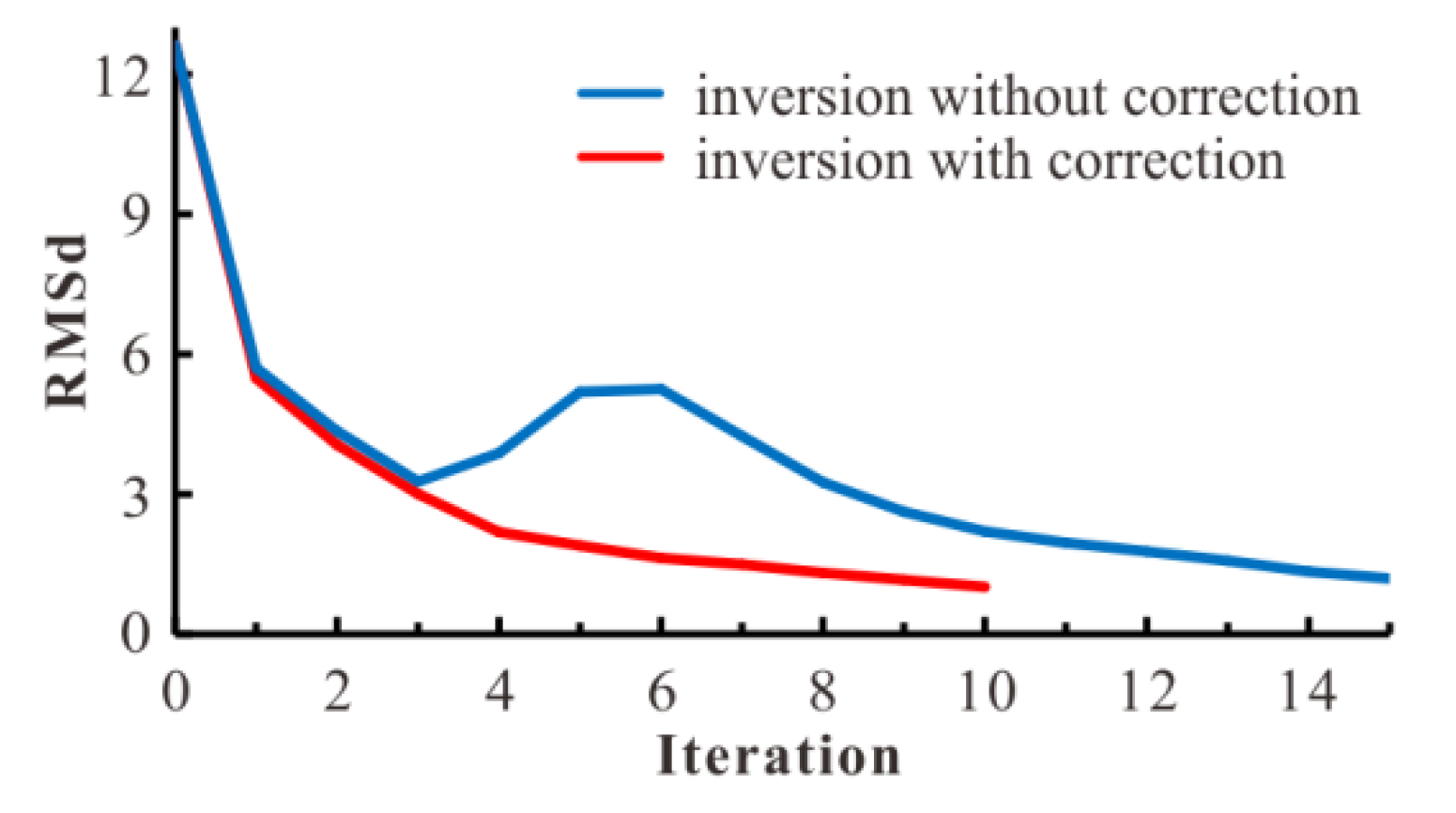
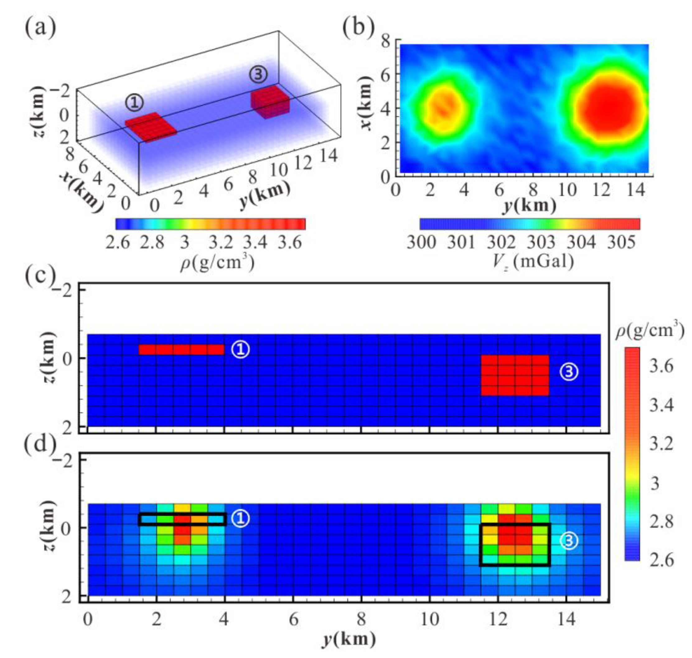
3.1. Effect Analysis of Element Volume Correction

In this section, we verified the effectiveness of our correction of sensitivity-based weighting through gravity inversion tests. As shown in Figure 5a–c, the model with a background density of 2.67 g/cm³ was divided into 16 × 30 × 10 elements. There were three abnormal bodies with a density of 3.67 g/cm³ in this model (Figure 5b), and the observation plane containing 16 × 30 points was located at z = −2200 m. Random noise with a normal distribution was added to the synthetic data (Figure 5d), and its intensity was 5% of the relative anomaly generated by body ③. The data were separately inverted without element volume correction and with correction. Although the data were observed airborne, we took r = 2 for both inversions because the observation plane was relatively close to the field sources. Other parameters of the two groups were also exactly the same, where Λ_m0 = 50.

In this paper, we used thick lines to mark the real anomaly boundaries in the inversion results as a reference and evaluated the results quantitatively by data misfit (RMSd) and model misfit (RMSm):

$$\mathrm{RMSd}=\sqrt{{\displaystyle \sum _{i=1}^N{\left(\frac{d_i^{obs}-d_i^{inv}}{er{r}_i}\right)}^2/N}},$$

(32)

$$\mathrm{RMSm}=100\times \sqrt{{\displaystyle \sum _{i=1}^M{\left(m_i^{true}-m_i^{inv}\right)}^2/M}},$$

(33)

where m^true and d^obs are the real model and observation data, m^inv and d^inv are the result model and its forward response, and err is the observation error. A smaller RMSd means a better data fitting, and a smaller RMSm indicates a higher degree of model restoration.

Although both groups successfully converged to the expected data misfit (Figure 6), the inversion with correction performed more smoothly. In the result without correction (Figure 7b), the anomalies of body ③ were wrongly gathered to the small elements near the surface, and some anomalies of body ② were also induced into the small elements below it. Conversely, the inversion carrying out the correction restored the underground better (Figure 7c), which is also indicated by the RMSm comparison in

Table 2. RMSm of gravity inversion results.

	Initial Model	Without Correction	With Correction
RMSm_ρ	18.03	19.10	14.49

.

Notice that the body ① in Figure 7c seems to be reflected to a deeper position owing to the correction; we retained bodies ① and ③ to build a similar model under the regular grid (Figure 8a) and took the same observation surface, noise synthetic mode, and inversion parameters for it, with observation data that are presented in Figure 8b. The inversion result (Figure 8d) was basically consistent with the shapes of bodies ① and ③ in Figure 7c, which meant the correction almost corrected the influence of only the volume difference and rarely affected the normal regularization.

To further verify whether the volume correction would induce the anomalies of small elements out, we tested a model, as seen in Figure 9a, where two cuboids with the same size and density were buried at the same depth, and one of them was divided into smaller subelements. The noise synthetic mode and inversion parameters remained consistent with the previous two models, but the observation plane was set on the surface. During the inversion process of the observation data (Figure 9b), the group with volume correction achieved better data fitting than the other group (Figure 9c). We learned from the density slices that whether the volume correction was carried out (Figure 9f) or not (Figure 9e), the body ② was well-restored, but the correction made body ① more accurate, which proved that our correction would not misrepresent the anomalies that should be in the small elements.

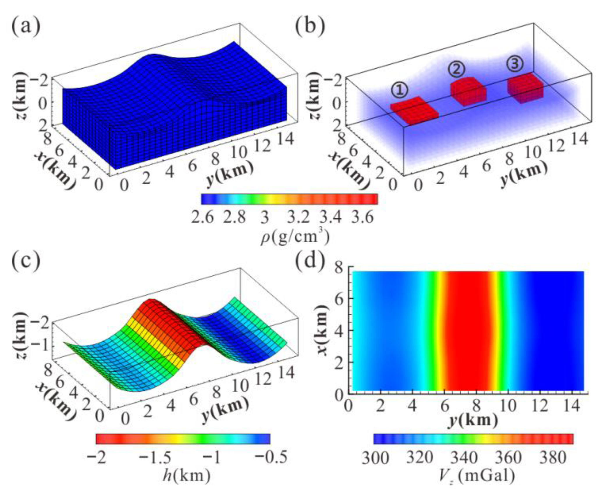
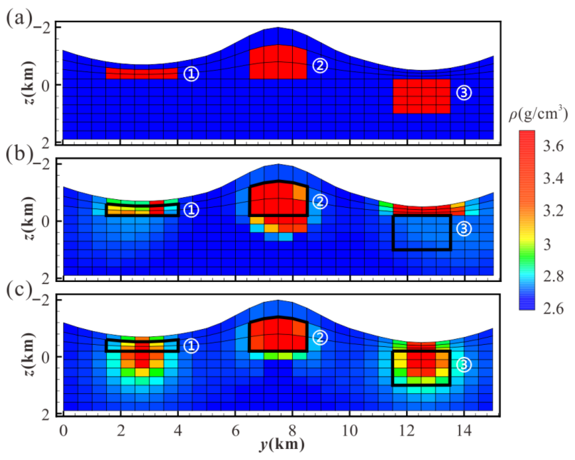
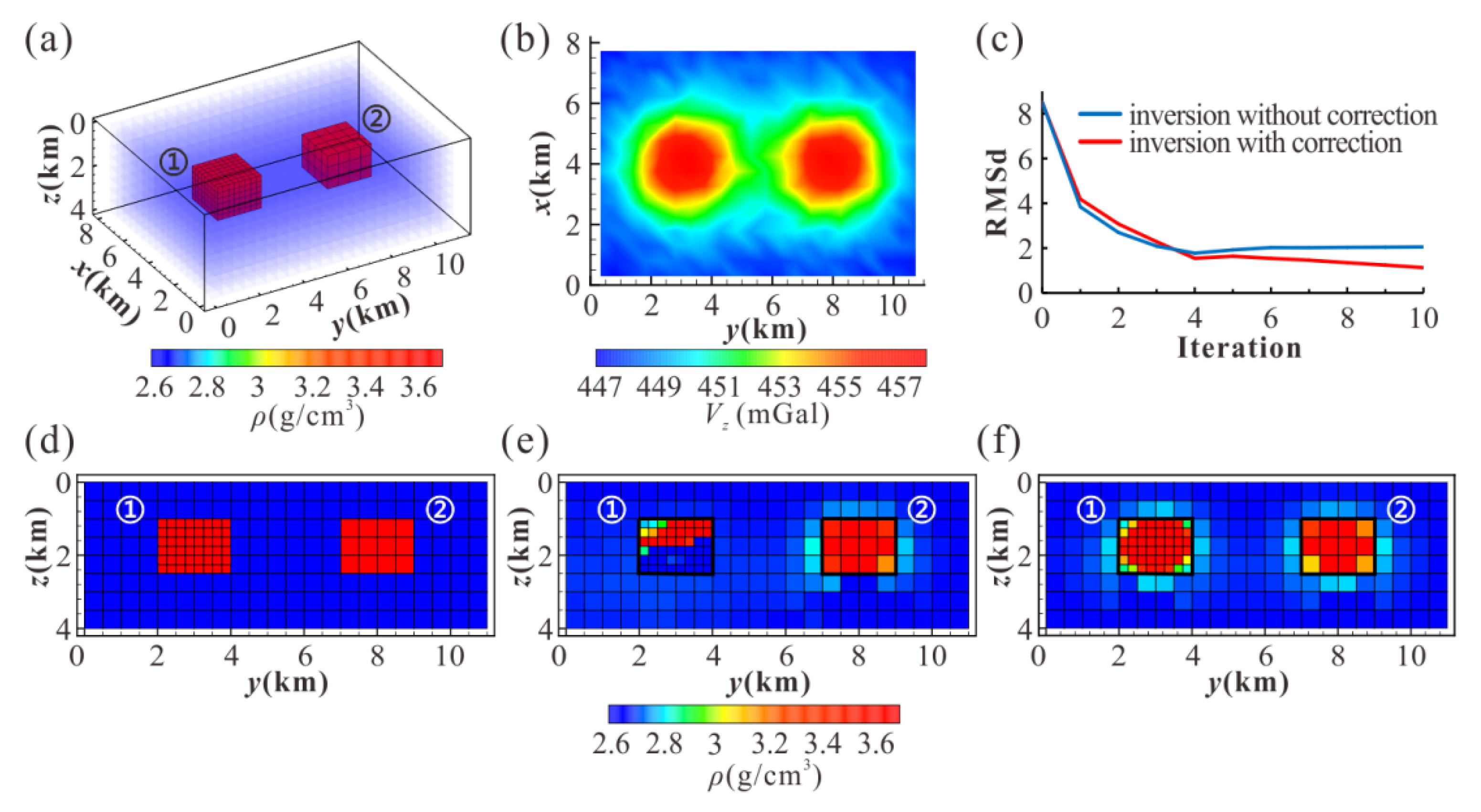
3.2. Effect Analysis of Joint Inversion Based on Combined Hexahedral Grid

In this section, we tested the cross-gradient joint inversion based on the combined hexahedral grid. As shown in Figure 10a–d, the model with a background density of 2.67 g/cm³ and magnetization of 1 A/m was divided into 22 × 22 × 14 hexahedrons. Magnetic inclination and declination were set to 60° and 90°. There were three abnormal bodies in this model, including ① an oblique step (3.67 g/cm³, 2 A/m), ② a horizontal cuboid (3.27 g/cm³, 2 A/m), and ③ a curved hexahedron (3.67 g/cm³, 2 A/m). The observation plane containing 22 × 22 points was located at z = −2500 m. Random noises with normal distributions were added to the synthetic data (Figure 10e,f), and their intensity was 5% of the corresponding relative anomaly generated by body ②. Then, we conducted separate inversions and cross-gradient joint inversions on the data under the tetrahedral grid (using Equations (23) and (24)) and the combined hexahedral grid, respectively. Since the observation plane was farther from the buried bodies compared with the previous section, we took r_ρ = 3 and r_κ = 2. For the consistency of model details, we subdivided each hexahedral element into six tetrahedrons, as shown in Figure 11, to construct the tetrahedral grid in this test.

To better compare the joint effectiveness of the two grids, it was necessary to ensure them similar separate results. Therefore, fixing the iteration times to 15, we tried several groups of Λ_m0ρ and selected the optimal one to meet this requirement. Finally, we took Λ_m0ρ = 10 and Λ_m0κ = 10 for the combined hexahedral grid and Λ_m0ρ = 3 and Λ_m0κ = 12 for the tetrahedral grid. The RMSd curves of the separate inversions are shown in Figure 12, and their result slices are presented in Figure 13b,d,g,i and Figure 14b,d,g,i. Though restoring the underground to a certain extent, these slices still lacked accuracy compared with the real situation (Figure 13a,f and Figure 14a,f), and their density and magnetization structures showed inconsistency.

To evaluate the joint effectiveness more intuitively, we defined a cross-gradient descent rate t_ratio:

$$t_{ratio}=\frac{t_{s\_sep}-t_{s\_joi}}{t_{s\_sep}}\times 100\%,$$

(34)

$$t_s={\Vert \sqrt{t_x^2+t_y^2+t_z^2}\Vert }_1,$$

(35)

where the subscripts sep and joi represent separate inversion and joint inversion. A higher t_ratio means the cross-gradient decreases to a greater extent. In addition, we also used the Pearson correlation coefficient to evaluate the overall similarity of the gravity and magnetic model, and a higher Pearson coefficient indicated a more similar result.

Keeping the same Λ_m0 as separate inversions, we used the magnetic model to constrain gravity unilaterally in joint inversions (Λ_j0κ = 0) for the convenience of comparison. Maintaining the iteration times at 15, we tried different Λ_j0ρ for the two groups of inversions (Figure 15) and took the attempt with the highest t_ratio as the final result. Their RMSd curves are also shown in Figure 12. Since there are actually no density constraints on magnetic joint inversions, their magnetization results (Figure 13h,j and Figure 14h,j) were consistent with their separate results (Figure 13g,i and Figure 14g,i). Judging from the result slices, the cross-gradient constraint brought some positive effects to both inversion groups. For example, the density boundaries between bodies in Figure 13c,e and Figure 14c,e became clearer than their separate results (Figure 13b,d and Figure 14b,d). Moreover, the density amplitude of body ② in Figure 14c,e was better recovered. The RMSm statistics and Pearson coefficients in

Table 3. RMSm of inversion results.

	Initial Model	Separate Result (Tetrahedral)	Joint Result (Tetrahedral)	Separate Result (Combined Hexahedral)	Joint Result (Combined Hexahedral)
RMSm_ρ	16.83	12.38	11.99	12.78	11.51
RMSm_κ	20.47	13.36	13.36	13.03	13.03

and

Table 4. Pearson correlation coefficients of inversion results.

	Real Model	Separate Result (Tetrahedral)	Joint Result (Tetrahedral)	Separate Result (Combined Hexahedral)	Joint Result (Combined Hexahedral)
Pearson coefficient	0.9687	0.8936	0.9420	0.8757	0.9577

also indicated that the cross-gradient constraint made the density structure more accurate and more consistent with magnetization. This information proved that the cross-gradient function works well under both grids.

However, the two joint inversions also presented many differences. First, it can be seen in Figure 15 that using the geometric sense “cross-gradient” in the combined hexahedral grid caused t to drop more effectively than using the spatial sense cross-gradient in the tetrahedral grid, which was consistent with our analysis in the theoretical part. Second, as seen in the result slices, the structure similarity jointed by the tetrahedral grid was also inferior to that of the hexahedral grid, such as the upper boundary of body ③ in Figure 13c,h and the lower boundary of body ③ in Figure 14c,h. Moreover, it can be seen in Table 4 that the Pearson coefficient of the hexahedral separate result was lower than that of the tetrahedral, but the hexahedral group obtained a higher Pearson coefficient than the tetrahedral group after cross-gradient constraint, which indicated that our method had a stronger constraint ability.

3.3. Efficiency Analysis of Joint Inversion Based on Combined Hexahedral Grid

Continuing the model test in Section 3.2, we further analyzed the efficiency of our algorithm by comparing it with the inversions based on the tetrahedral grid and complete curved hexahedral grid. The processor used in this test was the Inter Core i5-7200U, the RAM was 8 GB, and the software was MATLAB R2020a. Without considering the influence of memory on the computing performance, we estimated that the time cost was linear with the element number. Since the element number of the tetrahedral grid was six times that of the hexahedral grid, we divided its relevant time by six before recording, to balance the contrast.

For these algorithms, differences exist only in the calculation of sensitivity matrix J and cross-gradient correlation terms. In this test, the forward modeling of the 4-node tetrahedron was realized by the 4-node Hammer integral, the forward modeling of the 20-node curved hexahedron was realized by the 8-node Gauss integral, and the regular hexahedron was calculated by the analytical formula. We recorded the time cost of a single J calculation of the three algorithms in

Table 5. Time cost of a single calculation of sensitivity matrix.

	Tetrahedral Grid	Curved Hexahedral Grid	Combined Hexahedral Grid
gravity (s)	2.238	250.9	71.89
magnetic (s)	13.13	1160	329.1

. It can be seen that the forward time of the complete curved hexahedral grid was much higher than that of the tetrahedral grid, because the curved hexahedron used more nodes to simulate geometric shape and numerical integration, and its coupling between geometric nodes was more complex. Although more nodes usually mean higher simulation accuracy, this efficiency gap was too large. Our algorithm effectively narrowed this gap by replacing part of the curved hexahedrons with regular hexahedrons, which could be forwarded faster. Since the sensitivity of the gravity and magnetic data was independent of the physical parameters, the whole inversion process only needed to calculate J once. Therefore, this time cost difference would not be further expanded with the increase in the number of forward.

Then, we compared the efficiency of calculating cross-gradient correlation terms (

Table 6. Time cost of 1000 calculations of cross-gradient correlation terms.

	Tetrahedral Grid	Curved Hexahedral Grid	Combined Hexahedral Grid
time cost (s)	107.8	9.043	9.119

). Considering that a single calculation took little time, which made it vulnerable to errors, we performed 1000 consecutive calculations in each group. Obviously, the calculation efficiency of cross-gradient correlation terms in the hexahedral grid was much higher than that in the tetrahedral grid, because of its regular arrangement. Finally, we recorded the time cost of a complete inversion process with 20 iterations of the three algorithms in

Table 7. Time cost of complete inversion process.

	Tetrahedral Grid	Curved Hexahedral Grid	Combined Hexahedral Grid
time cost (s)	525.5	1900	887.2

. We inferred that the difference was caused mainly by the forward speed, and our algorithm based on the combined hexahedral grid ensured a certain efficiency as a whole.

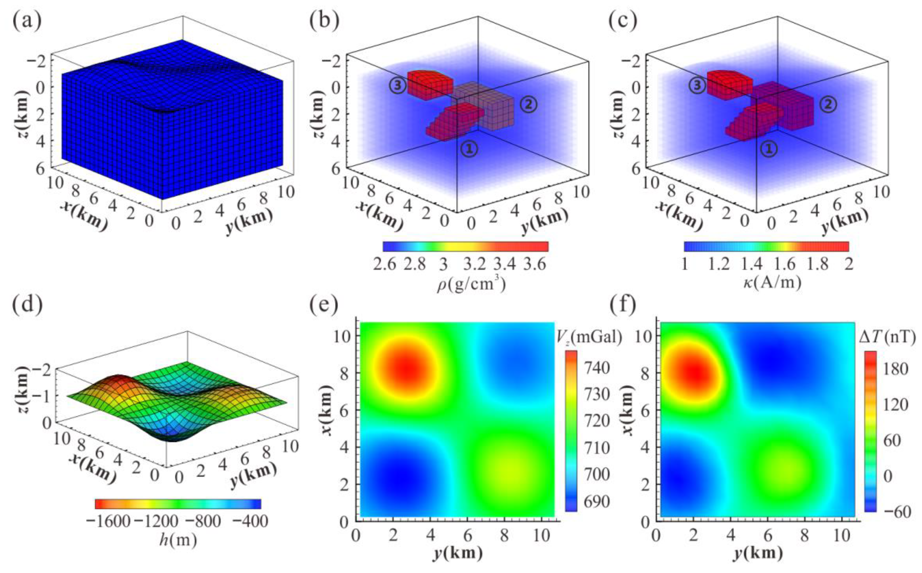
3.4. Effect Analysis of Application in Complex Terrain

In this section, we analyze the effectiveness of our combined hexahedral algorithm in a complex terrain condition. Due to the drawing software limitations, we used eight-node hexahedrons to represent curved hexahedrons. As shown in Figure 16a–d, the model with a background density of 2.67 g/cm³ and magnetization of 1 A/m was divided into 24 × 20 × 10 elements, and the magnetic inclination and declination were set to 70° and 60°. There were three abnormal bodies with high density (3.67 g/cm³) and high magnetization (2 A/m) in this model. The observation surface containing 24 × 20 points was set on the Earth’s surface. Random noises with normal distributions were added to the synthetic data (Figure 16e,f), and their intensity was 5% of the corresponding relative anomaly generated by body ①.

Then, we conducted separate inversion and joint inversion on the observation data, where r_ρ = 2, r_κ = 1, Λ_m0ρ = 50, Λ_m0κ = 10, Λ_j0ρ = 0.1, and Λ_j0κ = 0.1, and their RMSd curves are shown in Figure 17, converging successfully. We observed in the result slices that even in a complex terrain condition, joint inversion based on our geometric sense “cross-gradient” (Figure 18c,f) obtained more accurate and consistent results with both the gravity and magnetic data than with separate inversions (Figure 18b,e). For example, the boundary of body ① became more accurate, and the boundary between ② and ③ became clearer. This was also confirmed by the RMSm statistics and Pearson coefficients in

Table 8. RMSm of inversion results.

	Initial Model	Separate Inversion	Joint Inversion
RMSm_ρ	15.81	10.54	9.75
RMSm_κ	15.81	10.59	9.71

and

Table 9. Pearson correlation coefficients of inversion results.

	Real Model	Separate Inversion	Joint Inversion
Pearson coefficient	1	0.9117	0.9908

. Moreover, in the significant cross-gradient decline from the separate inversion (Figure 19a) to the joint inversion (Figure 19b), we noted that the constraint was robust.

This test further proved that our combined hexahedral algorithm could perform well in a complex terrain condition, where the sharp fluctuations may affect the shapes of adjacent elements. However, our grid also contained some limitations under severe topographic relief, that is, the elements below low terrain were too dense, which may cause a waste of computing resources.

3.5. Real Data Application

To test the practicability of our algorithm, we applied it to the measured data from a mining area in Huzhong, northwest Heilongjiang Province, China. The area (122°55′E, 52°13′N) is located in the Erguna polymetallic metallogenic belt, in the Greater Khingan Range, with an inclination of about 69.7° and a declination of about −11.35°. According to previous research, the Early Cambrian Wolegen Group-complex and the Early Cretaceous intrusive rocks supplied sufficient metallogenic materials, while the deep fracture of the Pangu-Kamalan River provided a place for the flow and precipitation of the metallogenic hydrothermal solution. Under frequent magmatic activity, the moderately acidic Early Cretaceous granite intruded into the marble of the Jixianggou formation, Wolegen Group-complex, forming abundant skarn type ore deposits with anomalies of high density and high magnetization [33].

After gridding a set of observations with 2 × 900 gravity and magnetic data, 30 × 30 measuring points were evenly distributed on the Earth’s surface, with spacing of 47.1 m in the X direction and 47.4 m in the Y direction. We, accordingly, divided the study area with the terrain in Figure 20b into a model with 30 × 30 × 20 elements under a local reference system (Figure 20a), with an expected spatial resolution that was about 47.1 m × 47.4 m × 50 m, and the center of each grid in the observation maps (Figure 20c,d) corresponded to a measuring point. Owing to the lack of topographic information around the area, we assumed that the elevation of a terrain node in the expansion zone was consistent with its nearest known elevation node. Considering that the gravity response of a model is related to its maximum depth when the background density is not 0, we added a horizontal background to the free-air anomaly as the gravity observation data (Figure 20c), to match our model. Since the magnetic response was not affected by the maximum depth of the model, the measured data without height correction were directly used as the magnetic observation data (Figure 20d). According to previous research, the location of a proven skarn deposit in this area was marked with a black star in Figure 20c,d. Then, taking the uniform half space with a density of 2.67 g/cm³ and magnetization of 0 A/m as the initial model, we conducted a separate inversion and joint inversion on the observation data, where r_ρ = 1.5, r_κ = 1, Λ_m0ρ = 50, Λ_m0κ = 50, Λ_j0ρ = 1, and Λ_j0κ = 0.1.

After several iterations, the RMSd of both inversion groups converged successfully (Figure 21), and the joint inversion took 33.9 min in total under the same computing environment as in Section 3.3. We performed two-dimensional slicing of the inversion results at z = −780 m and y = 750 m (Figure 22e and Figure 23e). As shown in Figure 22a,c and Figure 23a,c, there were obvious structural differences between the separate results of the gravity and magnetic data, so it was difficult to clearly delineate the boundary of the abnormal body, which was not conducive to the comprehensive interpretation of the study area. Meanwhile, under the cross-gradient constraint, the density result obtained higher consistency with magnetization (Figure 22b,d and Figure 23b,d). We used thick black lines to delineate the body with both high density and high magnetization in the joint result as the interpretation of skarn deposit and showed its three-dimensional perspective in Figure 24. The location of the inferred body was found to be consistent with the known deposit marked in Figure 20c,d, which further proved the effectiveness and practicability of our method.

4. Discussion

In this paper, we proposed a combined hexahedral grid for the joint inversion of the gravity and magnetic data, which supported a geometric sense “cross-gradient” to replace the traditional cross-gradient in the spatial sense. In addition, we further corrected the traditional sensitivity-based weighting function according to element volume to make it suitable for an unstructured grid. A series of model tests were performed to verify the reliability of the proposed methods.

Firstly, we verified the effectiveness of the element volume correction in Section 3.1. The experimental results indicated that the proposed correction was appropriate. It avoided the error of the traditional form, which causes the anomalies to accumulate more easily in small elements, while not causing the anomalies that should be in small elements to be misdirected outside due to over-correction, thus effectively solving the false anomaly problem. Secondly, we performed joint inversions on the same model using the tetrahedral grid and the combined hexahedral grid in Section 3.2, where our grid imposed cross-gradient constraints more strongly and better avoided the influence of approximation in gradient calculation. Then, the inversion efficiencies of three kinds of grids were compared in Section 3.3. Owing to the use of more geometrical and integral nodes, the curved hexahedral grid required much more time for forward modeling than the tetrahedral grid, but the strategy combining curved hexahedrons with regular hexahedrons effectively reduced this gap. Moreover, our grid took significantly less time to compute the cross-gradient term and its derivatives than the tetrahedral grid. The test in Section 3.4 further proved that our algorithm performed well in a complex terrain condition, where the sharp fluctuations affect the shapes of adjacent elements.

Finally, the algorithm was applied to the measured data from a mining area in Huzhong, northwest Heilongjiang Province, China. According to the distribution of the measuring points, we built a discrete model matching its resolution under the local reference system. Subsequently, under the constraint of the cross-gradient function, inversion results with higher structural consistency were obtained, which allowed us to delineate the bodies with both high density and high magnetization in two-dimensional slices and take skarn type minerals with the same physical characteristics as geological comparisons. We also depicted the interpretation results of the inferred ore body from a three-dimensional perspective and were pleased to find that its location was highly consistent with the proven skarn deposit, proving that our algorithm had certain practicability. This application case will provide reference and guidance for the exploration of similar situation.

It is worth mentioning that, in addition to the gravity and magnetic data, using the combined hexahedral grid can also be applied to the joint inversion of other geophysical methods, if the corresponding forward theories can be clarified.

5. Conclusions

Unstructured modeling is an effective approach to solving the terrain problem in gravity and magnetic joint inversion. However, because of the irregular arrangement and element volume difference in an unstructured grid, some commonly used constraint methods cannot be applied to unstructured modeling. In this paper, we proposed a grid method combining curved hexahedrons and regular hexahedrons. The grid supported a geometric sense “cross-gradient” owing to its regular arrangement, thereby reducing the influence of gradient approximation on joint inversion, which is unrealizable for a tetrahedral grid. At the same time, the grid simulated undulating terrain with more geometric nodes and ensured a certain efficiency. In addition, we proposed an element volume correction for the traditional sensitivity-based weighting function to make it suitable for unstructured grids. Four model tests and a successful application case verified the effectiveness and practicability of the proposed algorithm.

References

1. Okabe, M. Analytical expressions for gravity anomalies due to homogeneous polyhedral bodies and translations into magnetic anomalies. Geophysics 1979, 44, 730–741. [Google Scholar] [CrossRef]
2. Jahandari, H.; Farquharson, C.G. Forward modeling of gravity data using finite-volume and finite-element methods on unstructured grids. Geophysics 2013, 78, G69–G80. [Google Scholar] [CrossRef]
3. Jahandari, H.; Bihlo, A.; Donzelli, F. Forward modelling of gravity data on unstructured grids using an adaptive mimetic finite-difference method. J. Appl. Geophys. 2021, 190, 104340. [Google Scholar] [CrossRef]
4. Meng, Q.F.; Ma, G.Q.; Wang, T.H.; Xiong, S.Q. The Efficient 3D Gravity Focusing Density Inversion Based on Preconditioned JFNK Method under Undulating Terrain: A Case Study from Huayangchuan, Shaanxi Province, China. Minerals 2020, 10, 741. [Google Scholar] [CrossRef]
5. Carrillo, J.; Perez, F.; Marco, A.; Gallardo, L.A.; Schill, E. Joint inversion of gravity and magnetic data using correspondence maps with application to geothermal fields. Geophys. J. Int. 2022, 228, 1621–1636. [Google Scholar] [CrossRef]
6. Bosch, M.; Meza, R.; Jimenez, R.; Hoenig, A. Joint gravity and magnetic inversion in 3D using Monte Carlo methods. Geophysics 2006, 71, G153–G156. [Google Scholar] [CrossRef]
7. Kamm, J.; Lundin, I.A.; Bastani, M.; Sadeghi, M.; Pedersen, L.B. Joint inversion of gravity, magnetic, and petrophysical data; a case study from a gabbro intrusion in Boden, Sweden. Geophysics 2015, 80, B131–B152. [Google Scholar] [CrossRef]
8. Gallardo, L.A.; Meju, M.A. Characterization of heterogeneous near-surface materials by joint 2D inversion of dc resistivity and seismic data. Geophys. Res. Lett. 2003, 30, 1658. [Google Scholar] [CrossRef]
9. Gallardo, L.A.; Meju, M.A. Joint two-dimensional DC resistivity and seismic travel time inversion with cross-gradients constraints. J. Geophys. Res. Solid Earth 2004, 109, B03311-n/a. [Google Scholar] [CrossRef]
10. Pak, Y.C.; Li, T.L.; Kim, G.S. 2D data-space cross-gradient joint inversion of MT, gravity and magnetic data. J. Appl. Geophys. 2017, 143, 212–222. [Google Scholar] [CrossRef]
11. Shi, Z.J.; Hobbs, R.W.; Moorkamp, M.; Tian, G.; Jiang, L. 3-D cross-gradient joint inversion of seismic refraction and DC resistivity data. J. Appl. Geophys. 2017, 141, 54–67. [Google Scholar] [CrossRef]
12. Gao, J.; Zhang, H.J. An efficient sequential strategy for realizing cross-gradient joint inversion; method and its application to 2-D cross borehole seismic traveltime and DC resistivity tomography. Geophys. J. Int. 2018, 213, 1044–1055. [Google Scholar] [CrossRef]
13. Fregoso, E.; Gallardo, L.A. Cross-gradients joint 3D inversion with applications to gravity and magnetic data. Geophysics 2009, 74, L31–L42. [Google Scholar] [CrossRef]
14. Zhou, J.J.; Meng, X.H.; Guo, L.H.; Zhang, S. Three-dimensional cross-gradient joint inversion of gravity and normalized magnetic source strength data in the presence of remanent magnetization. J. Appl. Geophys. 2015, 119, 51–60. [Google Scholar] [CrossRef]
15. Joulidehsar, F.; Moradzadeh, A.; Ardejani, F.D. An Improved 3D Joint Inversion Method of Potential Field Data Using Cross-Gradient Constraint and LSQR Method. Pure Appl. Geophys. 2018, 175, 4389–4409. [Google Scholar] [CrossRef]
16. Zhang, R.Z.; Li, T.L.; Liu, C.; Huang, X.G.; Jensen, K.; Sommer, M. 3-D Joint Inversion of Gravity and Magnetic Data Using Data-Space and Truncated Gauss-Newton Methods. IEEE Geosci. Remote Sens. Lett. 2021, 19, 1–5. [Google Scholar] [CrossRef]
17. Tavakoli, M.; Nejati Kalateh, A.; Rezaie, M.; Gross, L.; Fedi, M. Sequential joint inversion of gravity and magnetic data via the cross-gradient constraint. Geophys. Prospect. 2021, 69, 1542–1559. [Google Scholar] [CrossRef]
18. Vatankhah, S.; Liu, S.; Renaut, R.A.; Hu, X.Y.; Hogue, J.D.; Gharloghi, M. An Efficient Alternating Algorithm for the L-Norm Cross-Gradient Joint Inversion of Gravity and Magnetic Data Using the 2-D Fast Fourier Transform. IEEE Trans. Geosci. Remote Sens. 2022, 60, 1–16. [Google Scholar] [CrossRef]
19. Ozyildirim, O.; Demirci, I.; Gundogdu, N.Y.; Candansayar, M.E. Two dimensional joint inversion of direct current resistivity and radiomagnetotelluric data based on unstructured mesh. J. Appl. Geophys. 2020, 172, 103885. [Google Scholar] [CrossRef]
20. Lelievre, P.G.; Farquharson, C.G.; Hurich, C.A. Joint inversion of seismic traveltimes and gravity data on unstructured grids with application to mineral exploration. Geophysics 2012, 77, K1–K15. [Google Scholar] [CrossRef]
21. Jordi, C.; Doetsch, J.; Guenther, T.; Schmelzbach, C.; Maurer, H.; Robertsson, J.O.A. Structural joint inversion on irregular meshes. Geophys. J. Int. 2020, 220, 1995–2008. [Google Scholar] [CrossRef]
22. Yin, C.C.; Sun, S.Y.; Gao, X.H.; Liu, Y.H.; Chen, H. 3D joint inversion of magnetotelluric and gravity data based on local correlation constraints. Acta Geophys. Sin. 2018, 61, 358–367. [Google Scholar] [CrossRef]
23. Lelievre, P.G.; Farquharson, C.G. Gradient and smoothness regularization operators for geophysical inversion on unstructured meshes. Geophys. J. Int. 2013, 195, 330–341. [Google Scholar] [CrossRef]
24. Mehanee, S.; Golubev, N.; Zhdanov, M.S. Weighted regularized inversion of magnetotelluric data. SEG Annu. Meet. Expand. Tech. Program Abstr. Biogr. 1998, 68, 481–484. [Google Scholar]
25. Li, Y.; Oldenburg, D.W. Joint inversion of surface and three-component borehole magnetic data. Geophysics 2000, 65, 540–552. [Google Scholar] [CrossRef]
26. Kim, K.; Hu, X.Y.; Cho, G.; Nam, M.; Kang, J.; Kim, G.; Liu, H. Study on isoparametric finite-element integral algorithm of gravity and magnetic anomaly for a body with complex shape. Shiyou Diqiu Wuli Kantan 2009, 44, 231–239. [Google Scholar]
27. Nagy, D. The gravitational attraction of a right rectangular prism. Geophysics 1966, 31, 362–371. [Google Scholar] [CrossRef]
28. Bhattacharyya, B.K. Magnetic anomalies due to prism-shaped bodies with arbitrary polarization. Geophysics 1964, 29, 517–531. [Google Scholar] [CrossRef]
29. Last, B.J.; Kubik, K. Compact gravity inversion. Geophysics 1983, 48, 713–721. [Google Scholar] [CrossRef]
30. Portniaguine, O.; Zhdanov, M.S. Focusing geophysical inversion images. Geophysics 1999, 64, 874–887. [Google Scholar] [CrossRef]
31. Portniaguine, O.; Zhdanov, M.S. 3-D magnetic inversion with data compression and image focusing. Geophysics 2002, 67, 1532–1541. [Google Scholar] [CrossRef]
32. Sampietro, D.; Capponi, M. Practical tips for 3D regional gravity inversion. Geophysics 2019, 9, 351. [Google Scholar] [CrossRef] [Green Version]
33. Li, S.P.; Li, T.L.; Zheng, J.; Chen, H.B.; Zhang, Z.Y. Application of 3D inversion of gravity magnetism electric method in upper mining area of Xiagalai Aoyi River. Glob. Geol. 2020, 39, 437–443. [Google Scholar]
Figure 1. Domain transformation of a 20-node curved hexahedron.
Remotesensing 14 04651 g001
Figure 2. Schematic diagram of combined hexahedral grid.
Remotesensing 14 04651 g002
Figure 3. Schematic diagram of terrain simulation from a two-dimensional perspective. (a) Using curved hexahedrons; (b) using tetrahedrons.
Remotesensing 14 04651 g003
Figure 4. Vertical view of the expansion zone.
Remotesensing 14 04651 g004
Figure 5. (a) Model division; (b) real density model; (c) topographic relief; (d) observation data.
Remotesensing 14 04651 g005
Figure 6. RMSd of gravity inversion.
Remotesensing 14 04651 g006
Figure 7. Density slice at x = 4000 m. (a) Real model; (b,c) inversion result without/with correction.
Remotesensing 14 04651 g007
Figure 8. (a) Real density model; (b) observation data; (c,d) density slice of the real model and inversion result at x = 4000 m.
Remotesensing 14 04651 g008
Figure 9. (a) Real density model; (b) observation data; (c) RMSd of inversion; (df) density slice of the real model and inversion result without/with volume correction at x = 4000 m.
Remotesensing 14 04651 g009
Figure 10. (a) Model division; (b,c) real density/magnetization model; (d) topographic relief; (e,f) observation data.
Remotesensing 14 04651 g010
Figure 11. Hexahedron subdivided into tetrahedrons.
Remotesensing 14 04651 g011
Figure 12. RMSd of inversion. (a) RMSd of gravity; (b) RMSd of magnetic.
Remotesensing 14 04651 g012
Figure 13. Slice of density (up) and magnetization (down) at y = 3500 m. (a,f) Real model; (b,g) separate result under tetrahedral grid; (c,h) joint result under tetrahedral grid; (d,i) separate result under combined hexahedral grid; (e,j) joint result under combined hexahedral grid.
Remotesensing 14 04651 g013
Figure 14. Slice of density (up) and magnetization (down) at x = 7500 m. (a,f) Real model; (b,g) separate result under tetrahedral grid; (c,h) joint result under tetrahedral grid; (d,i) separate result under combined hexahedral grid; (e,j) joint result under combined hexahedral grid.
Remotesensing 14 04651 g014
Figure 15. Cross-gradient descent rate of joint inversion under different Λj0ρ.
Remotesensing 14 04651 g015
Figure 16. (a) Model division; (b,c) real density/magnetization model; (d) topographic relief; (e,f) observation data.
Remotesensing 14 04651 g016
Figure 17. RMSd of inversion. (a) RMSd of gravity; (b) RMSd of magnetic.
Remotesensing 14 04651 g017
Figure 18. Slice of density (up) and magnetization (down) at y = 5000 m. (a,d) Real model; (b,e) separate result; (c,f) joint result.
Remotesensing 14 04651 g018
Figure 19. Cross-gradient of inversion result. (a) Separate result; (b) joint result.
Remotesensing 14 04651 g019
Figure 20. (a) Model division; (b) topographic relief; (c,d) observation data. The black stars indicate the location of the proven skarn deposit.
Remotesensing 14 04651 g020
Figure 21. RMSd of inversion. (a) RMSd of gravity; (b) RMSd of magnetic.
Remotesensing 14 04651 g021
Figure 22. Slice of density (up) and magnetization (down) at z = −780 m. (a,c) Separate result; (b,d) joint result; (e) trace of slice.
Remotesensing 14 04651 g022
Figure 23. Slice of density (up) and magnetization (down) at y = 750 m. (a,c) Separate result; (b,d) joint result; (e) trace of slice.
Remotesensing 14 04651 g023
Figure 24. Interpretation of skarn deposit in three dimensions.
Remotesensing 14 04651 g024