Abstract
The development of multi-component seismic acquisition technology creates new possibilities for the high-precision imaging of complex media. Compared to the scalar acoustic wave equation, the elastic wave equation takes the information of P-waves, S-waves, and converted waves into account simultaneously, enabling accurate description of actual seismic propagation. However, inherent attenuation is one of the important factors that restricts multi-component high-precision migration imaging. Its influence is mainly reflected in the following three ways: first, the attenuation of the amplitude energy makes the deep structure display unclear; second, phase distortion introduces errors to the positioning of underground structures; and third, the loss of high frequency components reduces imaging resolution. Therefore, it is crucial to fully consider the absorption and attenuation characteristics of the real Earth during seismic modeling and imaging. This paper aims to develop an accurate attenuation compensation reverse-time migration scheme for complex heterogeneous viscoelastic media. We first utilize a novel viscoelastic wave equation with decoupled fractional Laplacians to depict the Earth’s attenuation behavior. Then, an adaptive stable attenuation compensation operator is developed to realize high-precision attenuation compensation imaging. Several synthetic and field data analyses verify the effectiveness of the proposed method.
1. Introduction
Multi-component seismic acquisition and processing technology has come to the foreground in recent years. Compared with traditional acoustic scalar seismic data, multi-component data contain richer wave field information, which enables detailed description of oil and gas reservoirs [,,,,,,]. To improve the imaging accuracy of multi-component seismic data, considerable attention has been paid to data preprocessing [], wave field separation [,], velocity model estimation [,], imaging conditions [,] and high-performance computing []. In addition to the above factors, the inherent attenuation of the Earth is also a major challenge faced by multi-component imaging [,,]. Its impact is mainly reflected in the following three effects: first, the attenuation of amplitude energy makes the deep structure display unclear; second, phase distortion introduces errors to the positioning of underground structures; and third, the loss of high-frequency components reduces the imaging resolution. Therefore, it is important to fully consider absorption and attenuation when undertaking seismic modeling and migration imaging.
Both laboratory experiments and field rock measurements have revealed that the real Earth shows almost frequency-independent attenuation behavior within the seismic frequency band []. The most common approach to considering attenuation in the time domain is based on mechanical (rheological) models, in which the frequency-independent attenuation is approximated by stacking mechanical units, e.g., the standard linear solid or Kelvin–Voigt elements []. However, such methods may not be suitable for large-scale Q-compensation reverse-time migration (Q-RTM) due to their large number of characterization parameters and high computational cost [,,]. Alternatively, a viscous wave equation with decoupled fractional Laplacians (DFL) has unique advantages in many respects. The amplitude term and phase term in the DFL viscous equation are expressed separately, and accurate Q-RTM results can be obtained by reversing the sign of the amplitude term [,,,]. Currently, DFL viscous wave equations are widely used in Q-compensation seismic imaging [,,,] and inversion [,,,].
In the context of Q-ERTM, one of the fundamental essentials is to reverse-amplify the absorbed energy to ameliorate imaging accuracy and the precision of deep structures. Zhu and Sun [] were the first to implement QERTM based on the DFL viscoelastic wave equation. Guo and McMechan [] proposed compensating for Q effects by adjoint-based least-squares reverse-time migration. However, the high-frequency noise contained in the seismic records is also exponentially amplified in this process, which can easily cause numerical instability. Although the low-pass filtering method ensures numerical stability [,,], its high-frequency cutoff threshold is fixed, so cannot flexibly adapt to medium changes and it is prone to excessive damage to high-frequency components. In recent years, some optimized stability compensation strategies have been proposed, e.g., regularization-operator-based schemes [], stabilization strategies by improving imaging conditions [,], and approaches based on iterative algorithms [,,]. Among them, Wang et al. [,,] proposed an adaptive stability compensation operator to maximize the high-frequency components while ensuring numerical stability by which the cutoff threshold is automatically determined according to the propagation time and the Q values of the medium. However, this adaptive stability term contains hybrid-domain operators (a function of space and wavenumber). For heterogeneous media, the average Q method (the fractional power terms are computed using an average Q instead of the real Q) is usually used to solve the hybrid-domain operator problem but this method actually has the effect of blurring Q, resulting in insufficient compensation accuracy.
In our previous study [], we proposed a novel viscoelastic wave equation with constant-order DFLs. This equation decouples the phase distortion and the amplitude attenuation effects, which facilitate the Q-RTM. More importantly, the hybrid-domain issue that plagued the original DFL equations is naturally avoided in our DFL viscoelastic wave equation, in which the order of the fractional Laplacian is fixed. Here, we use it as a forward engine, and further derive a mode-dependent adaptive stabilization operator. Although a large number of studies have contributed to Q-ERTM applying different concepts, some methods are still limited by compensation accuracy [], computational efficiency [] or model complexity []. In contrast, the proposed method achieves a more effective tradeoff between numerical stability and imaging accuracy. In contrast to the original adaptive stability approach [], the power term in the proposed stability operator is spatial-independent, thus it meets the imaging requirements of complex heterogeneous media in an efficient manner.
The paper is arranged as follows: We start by reviewing the constant-order DFL viscoelastic wave equation []. Next, we present a vector-separation-based P- and S-wave decouple method. We then describe the derivation of the proposed adaptive stabilization operator in detail and embed it into the framework of Q-compensation viscoelastic reverse time migration (Q-ERTM). In a section on numerical examples, two synthetic examples and a field data application are employed to demonstrate the accuracy and the advantages of the proposed Q-ERTM scheme. Finally, we provide a summary and conclusions.
2. Theory and Methods
2.1. Viscoelastic Wave Equation with Constant-Order DFLs
Starting from an approximated dispersion relation of constant Q model [], a novel viscoelastic wave equation with constant-order fractional Laplacians [] is established, which is written as:
where , and denote the stress components, and represent the particle velocity, and
where or corresponds to P- or S-wave, and attenuation strength . refers to the propagation velocity that is defined as , where represents the phase velocity at frequency . It is worth mentioning that, in Equation (2), two terms including control the amplitude decay, while the rest are phase-dominated terms. Unlike the original, for the DFL viscoelastic wave equation that contains hybrid-domain Laplacian operators, as shown in Equation (2), the wavenumber k has constant power (i.e., does not vary across space). Thus, taking it as the forward engine in Q-ERTM, this can guarantee simulation accuracy when handling heterogeneous Q media. The derivation and advantages of this equation can be found in Wang et al. [].
2.2. Separation of P- and S- Wavefields
Multi-component seismic data simultaneously contain P-wave, S-wave and converted-wave components. If the coupled wavefields are directly introduced into the migration process for imaging, serious crosstalk noise between different wave components will be generated. Thus, it is essential to separate the P- and S-wavefields during seismic extrapolation. The early separation scheme is based on Helmholtz theory, in which the divergence and curl operators are applied to separate the coupled wavefields [,]. However, this scheme will introduce amplitude distortion and phase-reversal to the separation results, causing the final migration results to lose physical meaning. To overcome this phenomenon, a vector-separation-based P- and S-wave decouple method is proposed to ensure that the actual vector characteristics remain unchanged [,]. Similar to Wang et al. [], we carry out wave field separation by introducing an intermediate variable , which satisfies:
It has the same physical meaning as the scalar acoustic pressure in the viscoacoustic wave equation. From the above equation, we can obtain a series of equations to perform P- and S-wave vector-decomposition:
The superscripts p and s represent the P- and S-components of stress or particle velocity, respectively. Using Equations (3)–(7), we realize the independent propagation of P- and S- waves during wavefield extrapolation.
2.3. Adaptive Stable Q-Compensation Scheme
As stated in previous studies, reversing the amplitude operator while keeping the dispersion operator unchanged produces a correct compensated wavefield when Q-ERTM is implemented using the DFL viscous wave equation []. Using a similar operation, Equation (2) becomes:
Equations (2) and (8) restore the correct amplitude and phase. The last major problem faced by Q-ERTM is numerical stability. Since seismic records usually contain high-frequency noise, they will also be exponentially amplified in the process of energy recovery, and eventually lead to numerical instability. Compared to the conventional filter-based stability scheme [], an adaptive stabilization operator [,,] has the potential to gain a better balance between numerical stability and imaging resolution. According to Wang et al. [], a mode-dependent adaptive stabilization has the following generalized form:
where represents the amplitude-attenuated operator. Combined with Equation (2), the amplitude-attenuated operator can be given by:
In Equation (9), is the introduced stabilization factor [], which can be empirically expressed as:
where is a man-made upper limit of compensation. The proposed scheme does not need to blur Q to avoid the hybrid-domain operator because the power terms of k in Equation (10) are constant. Thus, it has higher potential to enable “point-to-point” compensation for the attenuation over the existing scheme.
2.4. Implementation of Adaptive Stable Q-ERTM
The following process is used to achieve an adaptive stable Q-ERTM:
- (a)
- Forward propagating the source-wavefield.
With a wavelet estimated from seismic data (or a given wavelet), solving Equations (2)–(7), we obtain the attenuated pure P- and S- forward wavefield.
- (b)
- Backward propagating the receiver-wavefield.
With the reversed attenuated multi-components recorded data as the boundary condition to solve Equations (3)–(8), we obtain the compensated receiver wavefield. Note that the adaptive stabilization operator (Equation (9)) is implemented at each time-step iteration to maintain numerical stability.
- (c)
- Applying the imaging condition.
The Q-compensated image of the subsurface structure can be produced using the following source-normalized cross-correlation imaging conditions:
where the superscripts S and R correspond to the attenuated and compensated wavefield variables; and the subscripts P and S represent the P- and S-wave components, respectively.
3. Numerical Examples
3.1. Sample Sag Model
First, we conduct the proposed attenuation compensation algorithm for a simple sag model to verify its effectiveness. Figure 1 displays the P-wave velocity and quality factor model, respectively. We use the conversion formula , and to obtain the S-wave velocity and . The model contains 400 × 360 cells with a grid interval of 10 m. The simulation time is 1.5 s with a time step of 1.0 ms. There are 40 shots distributed evenly at a depth of 10 m. Each shot is recorded by 200 double-sided geophones. The source used is a Ricker wavelet with a dominant frequency of 15 Hz. Figure 2 shows the synthetic shot gathers corresponding to the elastic (Figure 2a) and viscoelastic (Figure 2b) media. As expected, the deep structural energy in the viscoelastic medium is obviously weakened due to the existence of attenuation. Figure 3a–c display the coupled wavefield, the decoupled P−component wavefield and the decoupled S−component wavefield of the 20th shot, respectively. We observe that the different components are separated accurately.
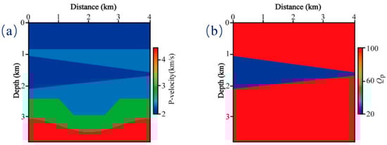
Figure 1.
Sag model. (a) P−wave velocity model and (b) P−wave quality factor model.
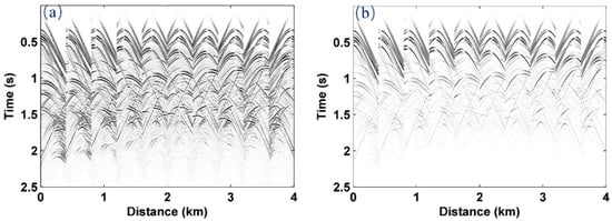
Figure 2.
Synthetic shot gathers corresponding to (a) the elastic media and (b) the loss media. Note that every 4th shot is shown.
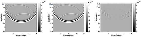
Figure 3.
The 20th snapshots. (a) the coupled wavefield, (b) the decoupled P−component wavefield and (c) the decoupled S−component wavefield.
Figure 4 and Figure 5 show the migrated PP− and PS-images, where we consider three scenarios: conventional ERTM from lossless seismic data (Figure 4a and Figure 5a), attenuated seismic data without compensation (Figure 4b and Figure 5b), and attenuated seismic data with the proposed Q-ERTM scheme (Figure 4c and Figure 5c). Note that there is a wedge-shaped high attenuation area in Figure 1b, and the imaging quality below this area is significantly worse (see Figure 4b and Figure 5b), which confirms the necessity of attenuation compensation. The Q-ERTM images match the reference well and the clearer structure and better horizontal continuity verify its effectiveness.
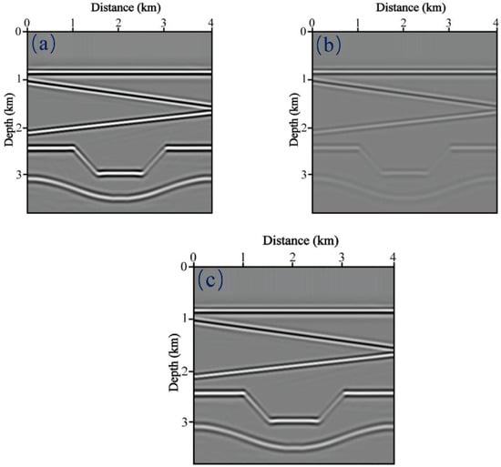
Figure 4.
PP−images of the Sag model obtained by (a) the conventional ERTM from lossless seismic data, (b) attenuated seismic data without compensation, (c) attenuated seismic data with the proposed Q-ERTM scheme.
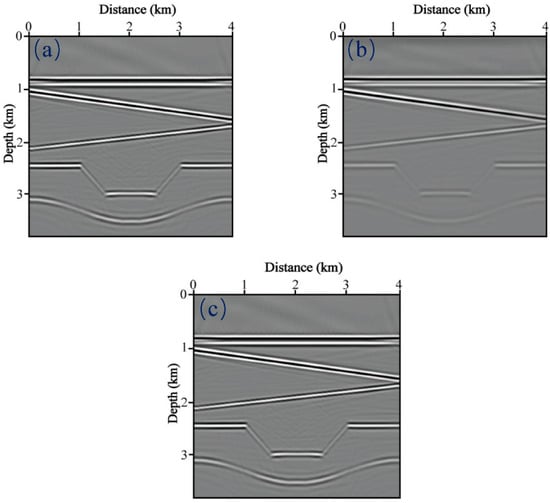
Figure 5.
PS-images of the Sag model obtained by (a) the conventional ERTM from lossless seismic data, (b) attenuated seismic data without compensation, (c) attenuated seismic data with the proposed Q-ERTM scheme.
3.2. Marmousi Model
We further employ a Marmousi model to show the compensation effect of the proposed method for complex heterogeneous media. Figure 6 displays the P−wave velocity and Q model. We also obtain the velocity and Q of S-wave through the conversion formula. This Marmousi model size is 234 × 640 with a spatial sampling interval of 10 m. There are 80 shots distributed evenly on the depth of 10 m. Each shot point has 160 bilateral records. The source we use is a Ricker wavelet with a dominant frequency of 30 Hz. The total calculation time is 2 s with a time-step of 1 ms. In this example, two different stabilization schemes are implemented: the low-pass-filter-based method and the proposed adaptive stabilization approach.
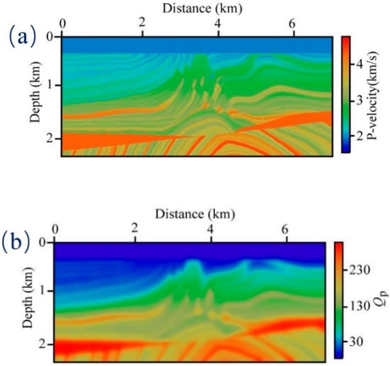
Figure 6.
The Marmousi (a) P−wave velocity and (b) quality factor model.
We show the migrated PP− and PS-images in Figure 7 and Figure 8 to demonstrate the compensation effect of the proposed method, where panels a–d correspond to the images using ERTM from lossless seismic data (reference solution), non-compensated images, compensated images with the low-pass filter, and compensated images with the proposed adaptively stabilized scheme, respectively. It is observed that the non-compensated migration (Figure 7b and Figure 8b) results exhibit obviously decreased resolution, weak energy of deep structure, and blurred structural details. For the low-pass-filter stabilization scheme, we only retain the components below 50 Hz to ensure numerical stability. Although the imaging quality is better than the non-compensated results, the resolution reduction caused by the loss of high-frequency information is obvious. The imaging results of the proposed scheme (Figure 7d and Figure 8d) look very close to the reference solution (Figure 7a and Figure 8a), which verifies the accuracy of compensation. It is worth mentioning that, due to the lower S-wave velocity, we observed that the PS images resolution is better than that of the PP images, which, to some extent, reflects the advantages of S-wave exploration. Figure 9 compares the traces extracted from the images generated by different migration algorithms at x = 4 km. It can be observed that the traditional low-pass filtering method (green line) is not sufficiently accurate to describe the deep structure, and both the amplitude and phase deviate from the reference trace (black line). In contrast, the proposed method (red line) can compensate for both P−wave and S-wave attenuation more accurately.
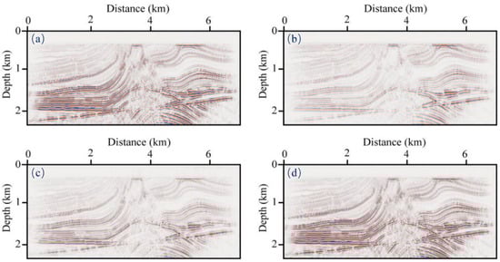
Figure 7.
PP−images generated by (a) ERTM from lossless seismic data (reference solution), (b) non-compensated images, (c) Q-compensated with low-pass filter, (d) Q-compensated with the proposed a stable scheme.
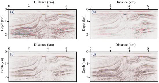
Figure 8.
PS-images generated by (a) ERTM from lossless seismic data (reference solution), (b) non-compensated images, (c) Q-compensated with low-pass filter, (d) Q-compensated with the proposed a stable scheme.
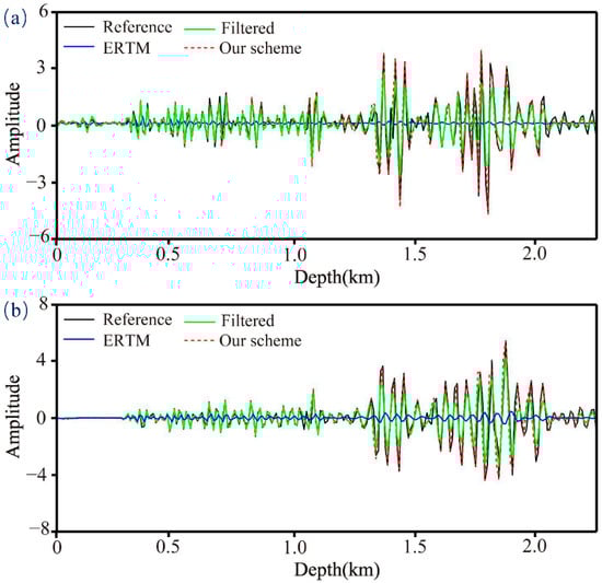
Figure 9.
Comparison of the traces at x = 4 km. (a) PP−component (b) PS-component.
3.3. Apply to Field Data
The above synthetic data fully verify the compensation effectiveness of the proposed method. In the last example, we demonstrate its applicability to field data. Figure 10a,b show the velocity and Q model of P−wave, respectively. We also obtain the velocity and Q of S-wave through the conversion formula. The model size is 10 km × 6 km with a spatial sampling interval of 20 m. There are 250 shots distributed laterally at the depth of 20 m. Before implementing migration, we preprocess the initial data with de-noise and surface wave suppression. The source wavelet we use is estimated from the seismic records. Figure 11a displays the 200th seismogram. As represented in the averaged amplitude spectrum shown in Figure 11b, the dominant frequency is almost 25 Hz.
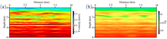
Figure 10.
The (a) P-wave velocity and (b) quality factor models correspond to the field data.
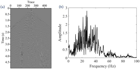
Figure 11.
(a) The observed seismogram selected from the 200th shot, (b) the corresponding amplitude spectrum.
We show the PP− and PS-images of non-compensated migration and Q-ERTM obtained by the proposed scheme in Figure 12. For the PP−images, we find poor lateral continuity and ambiguous deep-structure in the non-compensated migration (Figure 12a); while the imaging quality in the Q-ERTM profile is improved (see Figure 12b). As indicated by the arrows, the lateral continuity of the structure is significantly enhanced, and the deep-structure becomes clear. Speaking frankly, the PS−images are definitely more challenging due to the absence of accurate S−wave velocity and Q models. Although the PS−images are inferior to the PP-images, we still observe the improvement in the imaging quality of the proposed method (Figure 12d) over the traditional ERTM (Figure 12c). Figure 13 shows a comparison of the wavenumber spectra (selected from Figure 12 at the depth of 3 km); clearly, the proposed adaptive stable Q-ERTM scheme is able to retain more high-frequency information over the non-compensated ERTM migration.
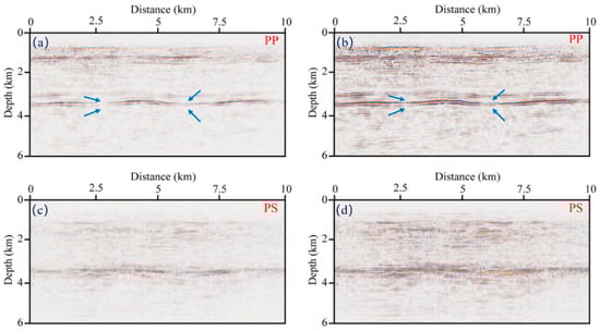
Figure 12.
PP-images of the field data obtained by (a) ERTM method (without Q-compensation), (b) the proposed Q-ERTM scheme; PS−images of the field data obtained by (c) ERTM method (without Q-compensation), (d) the proposed Q-ERTM scheme.
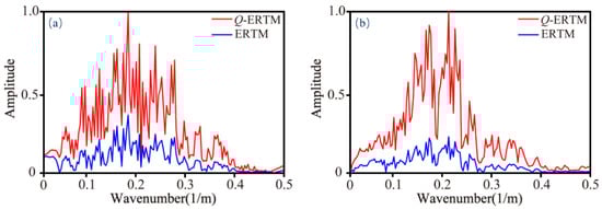
Figure 13.
Comparison of wavenumber spectra that are selected from Figure 12 at the depth of 3 km, (a) PP-component, (b) PS−component.
4. Conclusions
We developed an accurate attenuation compensation RTM scheme for complex heterogeneous viscoelastic media. We utilized a novel viscoelastic wave equation with constant-order fractional Laplacians as the forward engine to ensure simulation accuracy in complex attenuation media. Then, we derived a mode-dependent adaptive stabilization operator, in which the power term of the stability operator is spatial-independent, thus meeting the imaging requirements of complex heterogeneous media in an efficient manner. Two synthetic data analyses fully verify the compensation effectiveness of the proposed method, while a field data application further demonstrates its fidelity and stability. These numerical examples suggest that this adaptive, stable Q-ERTM scheme facilitates improvement in the description of complex structures in viscoelastic media.
Author Contributions
Conceptualization, N.W. and Y.S.; formal analysis, N.W. and H.Z.; methodology, N.W.; software, N.W.; supervision, Y.S. and H.Z.; writing—original draft, N.W.; writing—review and editing, H.Z. All authors have read and agreed to the published version of the manuscript.
Funding
This work is partly supported by the Open Funds of National Engineering Laboratory for Offshore Oil Exploration (CCL2020RCPS0420RQN), the National Natural Science Foundation of China (41930431, U19B6003-04, 42204129), the R&D Department of the China National Petroleum Corporation (2022DQ0604-03), and the Joint Guiding Project of the Natural Science Foundation of Heilongjiang Province (LH2021D009).
Data Availability Statement
The data used in this study is available by contacting the corresponding author.
Conflicts of Interest
The authors declare no conflict of interest.
References
- Du, Q.; Zhu, Y.; Ba, J. Polarity reversal correction for elastic reverse time migration. Geophysics 2012, 77, S31–S41. [Google Scholar] [CrossRef]
- Duan, Y.; Sava, P. Scalar imaging condition for elastic reverse time migration. Geophysics 2015, 80, S127–S136. [Google Scholar] [CrossRef]
- Nguyen, B.D.; McMechan, G.A. Five ways to avoid storing source wavefield snapshots in 2D elastic prestack reverse time migration. Geophysics 2015, 80, S1–S18. [Google Scholar] [CrossRef]
- Luo, J.; Wang, B.; Wu, R.S.; Gao, J. Elastic full waveform inversion with angle decomposition and wavefield decoupling. IEEE Trans. Geosci. Remote Sens. 2020, 59, 871–883. [Google Scholar] [CrossRef]
- Zhang, Y.; Liu, Y.; Xu, S. Viscoelastic Wave Simulation with High Temporal Accuracy Using Frequency-Dependent Complex Velocity. Surv. Geophys. 2021, 42, 97–132. [Google Scholar] [CrossRef]
- Zhang, W.; Gao, J.; Cheng, Y.; Su, C.; Liang, H.; Zhu, J. 3-D Image-Domain Least-Squares Reverse Time Migration with L1 Norm Constraint and Total Variation Regularization. IEEE Trans. Geosci. Remote Sens. 2022, 60, 5918714. [Google Scholar] [CrossRef]
- Huang, X.; Greenhalgh, S.; Han, L.; Liu, X. Generalized Effective Biot Theory and Seismic Wave Propagation in Anisotropic, Poroviscoelastic Media. J. Geophys. Res. Solid Earth 2022, 127, e2021JB023590. [Google Scholar] [CrossRef]
- Wang, C.; Wang, Y.; Wang, X.; Xun, C. Multicomponent seismic noise attenuation with multivariate order statistic filters. J. Appl. Geophys. 2016, 133, 70–81. [Google Scholar] [CrossRef]
- Xiao, X.; Leaney, W.S. Local vertical seismic profiling (VSP) elastic reverse-time migration and migration resolution: Salt-flank imaging with transmitted P-to-S waves. Geophysics 2010, 75, S35–S49. [Google Scholar] [CrossRef]
- Li, Z.; Ma, X.; Fu, C.; Liang, G. Wavefield separation and polarity reversal correction in elastic reverse time migration. J. Appl. Geophys. 2016, 127, 56–67. [Google Scholar] [CrossRef]
- Fang, J.; Chen, H.; Zhou, H.; Zhang, Q.; Wang, L. Three-dimensional elastic full-waveform inversion using temporal fourth-order finite-difference approximation. IEEE Geosci. Remote. Sens. Lett. 2021, 19, 1–5. [Google Scholar] [CrossRef]
- Zhang, W.; Gao, J. Deep-learning full-waveform inversion using seismic migration images. IEEE Trans. Geosci. Remote Sens. 2022, 60, 5901818. [Google Scholar] [CrossRef]
- Du, Q.; Guo, C.; Zhao, Q.; Gong, X.; Wang, C.; Li, X.Y. Vector-based elastic reverse time migration based on scalar imaging condition. Geophysics 2017, 82, S111–S127. [Google Scholar] [CrossRef]
- Yan, R.; Xie, X.B. An angle-domain imaging condition for elastic reverse time migration and its application to angle gather extraction. Geophysics 2012, 77, S105–S115. [Google Scholar] [CrossRef]
- Zhang, Q.; Mao, W.; Chen, Y. Attenuating crosstalk noise of simultaneous-source least-squares reverse time migration with GPU-based excitation amplitude imaging condition. IEEE Trans. Geosci. Remote Sens. 2018, 57, 587–597. [Google Scholar] [CrossRef]
- Zhu, T.; Sun, J. Viscoelastic reverse time migration with attenuation compensation. Geophysics 2017, 82, S61–S73. [Google Scholar] [CrossRef]
- Yang, J.; Zhu, H. Viscoacoustic reverse time migration using a time-domain complex-valued wave equation viscoacoustic RTM. Geophysics 2018, 83, S505–S519. [Google Scholar] [CrossRef]
- Guo, P.; McMechan, G.A. Compensating Q effects in viscoelastic media by adjoint-based least-squares reverse time migration. Geophysics 2018, 83, S151–S172. [Google Scholar] [CrossRef]
- McDonal, F.; Angona, F.; Mills, R.; Sengbush, R.; Van Nostrand, R.; White, J. Attenuation of shear and compressional waves in Pierre shale. Geophysics 1958, 23, 421–439. [Google Scholar] [CrossRef]
- Liu, H.P.; Anderson, D.L.; Kanamori, H. Velocity dispersion due to anelasticity; implications for seismology and mantle composition. Geophys. J. Int. 1976, 47, 41–58. [Google Scholar] [CrossRef]
- Robertsson, J.O.A.; Blanch, J.O.; Symes, W.W. Viscoelastic finite-difference modeling. Geophysics 1994, 59, 1444–1456. [Google Scholar] [CrossRef]
- Savage, B.; Komatitsch, D.; Tromp, J. Effects of 3D attenuation on seismic wave amplitude and phase measurements. Bull. Seismol. Soc. Am. 2010, 100, 1241–1251. [Google Scholar] [CrossRef]
- Zhu, T.Y.; Carcione, J.M.; Harris, J.M. Approximating constant-Q seismic propagation in the time domain. Geophys. Prospect. 2013, 61, 931–940. [Google Scholar] [CrossRef]
- Wang, N.; Zhou, H.; Chen, H.M.; Xia, M.M.; Wang, S.C.; Fang, J.W.; Sun, P.Y. A constant fractional-order viscoelastic wave equation and its numerical simulation scheme. Geophysics 2018, 83, T39–T48. [Google Scholar] [CrossRef]
- Wang, N.; Zhu, T.; Zhou, H.; Chen, H.; Zhao, X.; Tian, Y. Fractional Laplacians viscoacoustic wavefield modeling with k-space-based time-stepping error compensating scheme. Geophysics 2020, 85, T1–T13. [Google Scholar] [CrossRef]
- Xing, G.; Zhu, T. Modeling frequency-independent Q viscoacoustic wave propagation in heterogeneous media. J. Geophys. Res. Solid Earth 2019, 124, 11568–11584. [Google Scholar] [CrossRef]
- Zhu, T.Y.; Bai, T. Efficient modeling of wave propagation in a vertical transversely isotropic attenuative medium based on fractional Laplacian. Geophysics 2019, 84, T121–T131. [Google Scholar] [CrossRef]
- Zhu, T.Y.; Harris, J.M.; Biondi, B. Q-compensated reverse time migration. Geophysics 2014, 79, S77–S87. [Google Scholar] [CrossRef]
- Li, Q.Q.; Zhou, H.; Zhang, Q.C.; Chen, H.M.; Sheng, S.B. Efficient reverse time migration based on fractional Laplacian viscoacoustic wave equation. Geophys. J. Int. 2016, 204, 488–504. [Google Scholar] [CrossRef]
- Wang, Y.; Harris, J.M.; Bai, M.; Saad, O.M.; Yang, L.; Chen, Y. An explicit stabilization scheme for Q-compensated reverse time migration. Geophysics 2022, 87, F25–F40. [Google Scholar] [CrossRef]
- Mu, X.; Huang, J.; Li, Z.; Liu, Y.; Su, L.; Liu, J. Attenuation Compensation and Anisotropy Correction in Reverse Time Migration for Attenuating Tilted Transversely Isotropic Media. Surv. Geophys. 2022, 43, 737–773. [Google Scholar] [CrossRef]
- Xue, Z.; Sun, J.; Fomel, S.; Zhu, T. Accelerating full-waveform inversion with attenuation compensation. Geophysics 2018, 83, A13–A20. [Google Scholar] [CrossRef]
- Chen, H.; Zhou, H.; Rao, Y. Source Wavefield Reconstruction in Fractional Laplacian Viscoacoustic Wave Equation-Based Full Waveform Inversion. IEEE Trans. Geosci. Remote Sens. 2021, 59, 6496–6509. [Google Scholar] [CrossRef]
- Yang, J.; Zhu, H.; Li, X.; Ren, L.; Zhang, S. Estimating p wave velocity and attenuation structures using full waveform inversion based on a time domain complex-valued viscoacoustic wave equation: The method. J. Geophys. Res. Solid Earth 2020, 125, e2019JB019129. [Google Scholar] [CrossRef]
- Xing, G.; Zhu, T. Decoupled Fréchet kernels based on a fractional viscoacoustic wave equation. Geophysics 2022, 87, T61–T70. [Google Scholar] [CrossRef]
- Ammari, H.; Bretin, E.; Garnier, J.; Wahab, A. Time-reversal algorithms in viscoelastic media. Eur. J. Appl. Math. 2013, 24, 565–600. [Google Scholar] [CrossRef]
- Wang, Y. A stable and efficient approach of inverse Q filtering. Geophysics 2002, 67, 657–663. [Google Scholar] [CrossRef]
- Qu, Y.; Huang, J.; Li, Z.; Guan, Z.; Li, J. Attenuation compensation in anisotropic least-squares reverse time migration. Geophysics 2017, 82, S411–S423. [Google Scholar] [CrossRef]
- Zhao, X.; Zhou, H.; Wang, Y.; Chen, H.; Zhou, Z.; Sun, P.; Zhang, J. A stable approach for Q-compensated viscoelastic reverse time migration using excitation amplitude imaging condition. Geophysics 2018, 83, S459–S476. [Google Scholar] [CrossRef]
- Sun, J.Z.; Zhu, T.Y.; Fomel, S. Viscoacoustic modeling and imaging using low-rank approximation. Geophysics 2015, 80, A103–A108. [Google Scholar] [CrossRef]
- Zhang, W.; Gao, J. Attenuation compensation for wavefield-separation-based least-squares reverse time migration in viscoelastic media. Geophys. Prospect. 2022, 70, 280–317. [Google Scholar] [CrossRef]
- Mu, X.; Huang, J.; Yang, J.; Guo, X.; Guo, Y. Least-squares reverse time migration in TTI media using a pure qP-wave equation. Geophysics 2020, 85, S199–S216. [Google Scholar] [CrossRef]
- Wang, Y.; Zhou, H.; Zhao, X.; Zhang, Q.; Chen, Y. Q-compensated viscoelastic reverse time migration using mode-dependent adaptive stabilization scheme. Geophysics 2019, 84, S301–S315. [Google Scholar] [CrossRef]
- Wang, Y.; Zhou, H.; Zhao, X.; Zhang, Q.; Zhao, P.; Yu, X.; Chen, Y. CuQ-RTM: A CUDA-based code package for stable and efficient Q-compensated reverse time migration CUDA-based Q-RTM. Geophysics 2019, 84, F1–F15. [Google Scholar] [CrossRef]
- Wang, Y.F.; Zhou, H.; Chen, H.M.; Chen, Y.K. Adaptive stabilization for Q-compensated reverse time migration. Geophysics 2017, 83, S15–S32. [Google Scholar] [CrossRef]
- Wang, N.; Xing, G.; Zhu, T.; Zhou, H.; Shi, Y. Propagating seismic waves in VTI attenuating media using fractional viscoelastic wave equation. J. Geophys. Res. Solid Earth 2022, 27, e2021JB023280. [Google Scholar] [CrossRef]
- Dellinger, J.; Etgen, J. Wave-field separation in two-dimensional anisotropic media. Geophysics 1990, 55, 914–919. [Google Scholar] [CrossRef]
- Yan, J.; Sava, P. Isotropic angle-domain elastic reverse-time migration. Geophysics 2008, 73, S229–S239. [Google Scholar] [CrossRef]
- Zhang, Q.; McMechan, G.A. 2D and 3D elastic wavefield vector decomposition in the wavenumber domain for VTI media. Geophysics 2010, 75, D13–D26. [Google Scholar] [CrossRef]
- Wang, W.; McMechan, G.A.; Zhang, Q. Comparison of two algorithms for isotropic elastic P and S vector decomposition. Geophysics 2015, 80, T147–T160. [Google Scholar] [CrossRef]
Publisher’s Note: MDPI stays neutral with regard to jurisdictional claims in published maps and institutional affiliations. |
© 2022 by the authors. Licensee MDPI, Basel, Switzerland. This article is an open access article distributed under the terms and conditions of the Creative Commons Attribution (CC BY) license (https://creativecommons.org/licenses/by/4.0/).