Deep Learning with Adaptive Attention for Seismic Velocity Inversion

Abstract

The subsurface velocity model is crucial for high-resolution seismic imaging. Although full-waveform inversion (FWI) is a high-accuracy velocity inversion method, it inevitably suffers from challenging problems, including human interference, strong nonuniqueness, and high computing costs. As an efficient and accurate nonlinear algorithm, deep learning (DL) has been used to estimate velocity models. However, conventional DL is insufficient to characterize detailed structures and retrieve complex velocity models. To address the aforementioned problems, we propose a hybrid network (AG-ResUnet) involving fully convolutional layers, attention mechanism, and residual unit to estimate velocity models from common source point (CSP) gathers. Specifically, the attention mechanism extracts the boundary information, which serves as a structural constraint in network training. We introduce the structural similarity index (SSIM) to the loss function, which minimizes the misfit between predicted velocity and ground truth. Compared with FWI and other networks, AG-ResUnet is more effective and efficient. Experiments on transfer learning and noisy data inversion demonstrate that AG-ResUnet makes a generalized and robust velocity prediction with rich structural details. The synthetic examples demonstrate that our method can improve seismic velocity inversion, contributing to guiding the imaging of geological structures.

1. Introduction

In seismic exploration, seismic imaging is one of the most commonly employed techniques for mapping the structure of the oil and gas reservoir, which contributes to further inferring reservoir characteristics (e.g., lithology, fluid- and fracture-property) [1,2,3,4]. A reliable macro-velocity model is a prerequisite for seismic imaging [5,6,7]. Velocity inversion methods mainly consist of stacking velocity analysis, migration velocity analysis, tomography, full-waveform inversion, and so on [8,9,10,11]. Full-waveform inversion (FWI) has become a promising method for estimating velocity models of complex structures [12,13,14,15,16].

FWI suffers from three main problems: strong nonlinearity, high computational cost, and inversion non-uniqueness [15]. Tarantola proposed a time-domain FWI based on generalized least squares, which addressed nonlinear inversion by linearization [17]. Considering the intrinsically nonlinear relationship between velocity and reflection coefficient, nonlinear optimization algorithms were used to establish the mapping between seismogram and velocity [18,19,20]. To improve the inversion efficiency, the frequency-domain FWI was developed [21,22]. Compared with the time domain, the frequency domain wavefield is decoupled. Therefore, multi-scale analysis was used in frequency-domain FWI [23,24]. The principle of this method is consecutively to use lower frequency information as the input to estimate the higher frequency part, finally yielding ideal results [25,26,27]. In order to address the non-uniqueness problem of inversion, Laplace-domain FWI was developed [28,29]. Because of the frequency insensitivity of the Laplace domain, it can obtain the long-wavelength velocity model from a simple initial model [30,31]. Although previous studies indicate that FWI has the potential to image complex structures precisely, the objective function of FWI is strongly nonlinear, and it inevitably suffers from the aforementioned issues.

Therefore, velocity inversion needs an efficient and robust method to build an accurate model. Deep learning (DL) has been applied successfully in computer vision [32,33,34,35], demonstrating excellent nonlinear processability. Motivated by this idea, numerous studies have applied DL successfully in seismic denoising [36,37,38], seismic data reconstruction [39,40,41], seismic data interpretation and attribute analysis [42,43,44], and so on. In velocity inversion disciplines, DL has served as an alternative method to FWI with high precision, robustness, and efficiency [45,46,47,48,49].

The loss function, network architecture, and data type are thoroughly studied to improve the inversion resolution of complex stratigraphic boundaries. Local structures and details are mainly impacted by loss function [50,51]. Li et al. and Liu et al. proposed a novel loss function that combines structural similarity index (SSIM) and L1 norm, contributing to improving the inversion resolution [52,53]. The SSIM, suitable for the human visual system (HVS), evaluates the similarity of two images through lightness, contrast, and structure [54]. In terms of network architecture, Wu and Lin employed convolutional neural networks (CNN) with conditional random fields (CRF) to precisely predict the fault structure [55]. Li et al. proposed fully connected layers to learn spatially aligned feature maps, which improved the inversion accuracy of spatial locations of geological targets [52]. In selecting input data, common source point (CSP) gathers are always fed into the network for training the parameters of a network. However, they have weak spatial correspondence with velocity models. Nowadays, common-imaging point gathers (CIG) have been utilized for network training instead of seismograms, simplifying the feature extraction and showing excellent velocity model building [56,57]. Although the modern DL algorithms improve the inversion efficiency and effect, the experimental results show that it is insufficient to characterize stratigraphic boundaries and geological structures [49].

Therefore, this study focuses on improving the construction boundary extraction ability of modern DL algorithms. Here, we present a hybrid network (AG-ResUnet) consisting of Unet [58], residual units [59], and attention gates [60]. To precisely estimate the geological structure details in the velocity model, we introduce SSIM to the loss function and utilize SSIM to evaluate the inversion. Unlike other full reference image quality assessments (FR-IQAs) that focus on the value difference of each pixel, SSIM pays more attention to the local structural information in images, which is of great importance in reconstructing the structural details. In this study, we first train the hybrid network by a mix loss function, consisting of mean square error (MSE) and SSIM, to optimize each pixel and local patch velocity misfits simultaneously. Second, we compare the training effect of the mix loss function and MSE loss function and demonstrate that the mix loss function plays a vital role in retrieving local structures. To illustrate the strength of our method, we further compare predictions of AG-ResUnet and other methods (e.g., FWI and other conventional networks). Finally, we conduct the transfer learning and noisy data inversion experiments. The results demonstrate the generalization and robustness of our method. The synthetic examples indicate that our method can provide high-resolution recovery of the complex velocity model, thus significantly improving seismic imaging.

2. Methodology

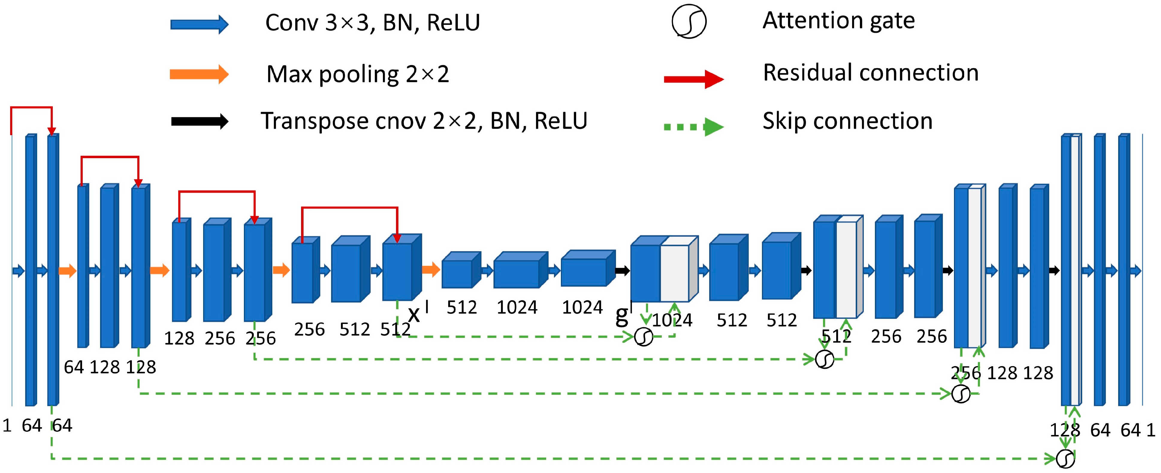
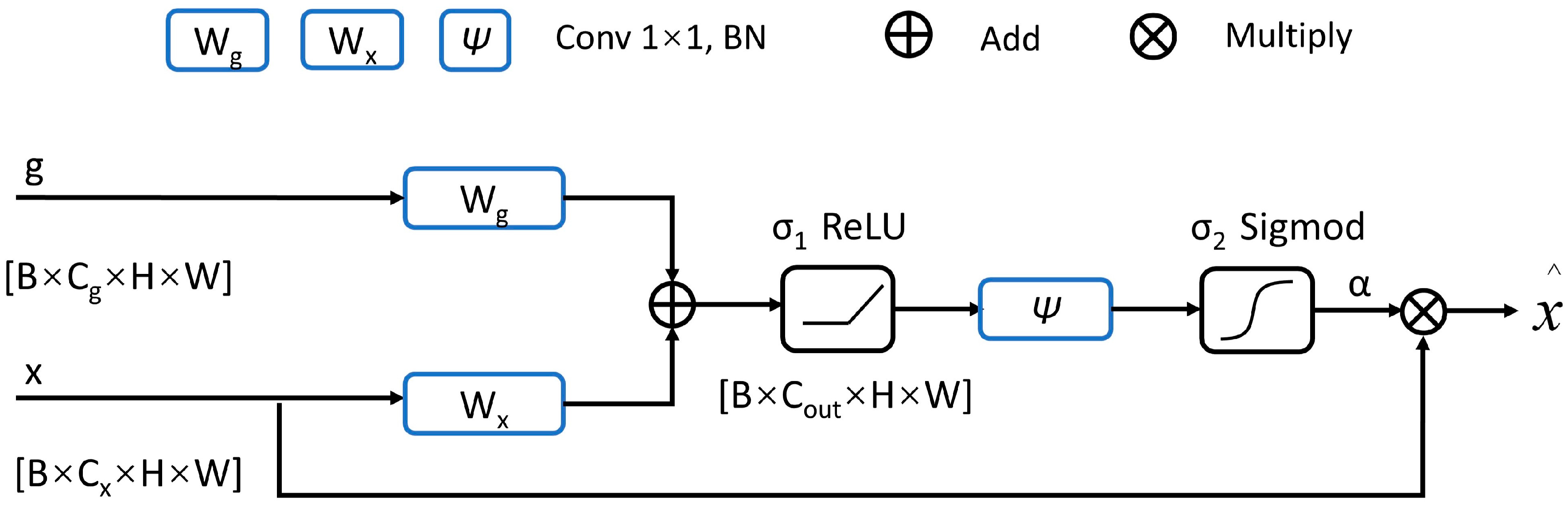
2.1. Network Architecture

The input of network is CSP gathers calculated from a 2D reference velocity model, and the output is the predicted velocity model. The AG-ResUnet consists of the Unet frame, residual unit, and attention gate (AG) (Figure 1). In Unet architecture, high-resolution features from the encoder combine with the decoder output (red arrow in Figure 1), avoiding direct supervision and loss computation in high-level feature maps. Although multiple convolutional layers can establish strongly nonlinear mappings between seismogram and velocity, the degradation problem of deep networks still poses a significant challenge. To tackle the degradation problem due to vanishing gradients, we introduce the residual skip connection (blue dotted line in Figure 1) between two non-adjacent layers in the encoder. By taking advantage of residual units, the network can continue learning new features with the vanishing of gradients.

AG (Figure 2), an attention mechanism, is employed in the medical segmentation, showing an excellent capability of boundary recognition [60]. Inspired by this idea, we utilize AGs in feature fusion, which adaptively focuses on the boundaries between geological targets. Its mathematical framework is as follows:

$$a^l={\sigma }_2\left({\Psi }^T\left({\sigma }_1\left(W_x^T{x}^l+W_g^T{g}^l+b_x+b_g\right)\right)+b_{\Psi }\right)$$

(1)

$$\widehat{x}=\alpha ·x$$

(2)

where $x^l$ is the low-level feature map at the l layer down-sampling, $g^l$ is the l layer up-sampling feature map, $W_x^T$, $W_g^T$, and ${\Psi }^T$ are $1\times 1$ convolutional layers, the superscript T means transpose, $b_x$, $b_g$, and $b_{\Psi }$ are bias terms, ${\sigma }_1$, ${\sigma }_2$ are ReLU and Sigmod activation functions, α is the gating coefficient, and $\widehat{x}$ is the feature map weighted by AG.

We take the addition of feature maps of x and g input into the nonlinear function ${\sigma }_1$ to obtain the output feature map. Then the channels of the output feature map are adjusted to one by the convolutional layer $\Psi$. Finally, the feature map values are limited between zero and one by ${\sigma }_2$, and multiply x to obtain the gating coefficient $\alpha$. The $\alpha$ value is higher at geological boundaries.

2.2. Loss Function

Mean-square error (MSE) is the most common loss function for regression problems (e.g., velocity inversion),

$$L_{MSE}\left(y_i,y_i^{\prime }\right)=\frac{1}{N}{\displaystyle \sum }_{i=1}^N{\left(y_i-y_i^{\prime }\right)}^2$$

(3)

where N denotes the total number of pixels in one single image, $y_i$ and $y_i^{\prime }$ represent velocity label and inversion velocity, respectively. $L_{MSE}$ minimizes the only pixel-wise distance between output and target and ignores the texture structures. Consequently, the local structural information, critical for achieving high-resolution subsurface models, would not be retrieved using $L_{MSE}$ only.

Local structures and details are vital factors to be focused on while recovering velocity models. To make the network optimization focus on local structural information, we introduce SSIM to the loss function. It describes the similarity of the two models from the perspective of local structure [54]. Evaluating model similarity with SSIM is known as full reference, meaning that a complete reference label (e.g., reference velocity models) is assumed to be known. The value of SSIM ranges from zero to one. The larger the value, the closer the predicted velocity model is to the ground truth. SSIM is defined as:

$$SSIM\left(y,y^{\prime }\right)=\frac{\left(2{\mu }_y{\mu }_{y^{\prime }}+C_1\right)\left(2{\sigma }_{y{y}^{\prime }}+C_2\right)}{\left({\mu }_y^2+{\mu }_{y^{\prime }}^2+C_1\right)\left({\sigma }_y^2+{\sigma }_{y^{\prime }}^2+C_2\right)}$$

(4)

where ${\mu }_y$ and ${\mu }_{y^{\prime }}$ represent the mean values of $y_i$ and $y_i^{\prime }$, respectively, ${\sigma }_y$ and ${\sigma }_{y^{\prime }}$ are the corresponding standard deviation, ${\sigma }_{y{y}^{\prime }}$ denotes the covariance of $y_i$ and $y_i^{\prime }$, and $C_1$ and $C_2$ represent constants to stabilize the division.

The combination of the MSE loss and the SSIM serves as a mix loss function ($L_{Mix}$) maintaining the advantages of both loss functions, which simultaneously optimize each pixel and local patch misfits,

$$L_{Mix}\left(y_i,y_i^{\prime }\right)=L_{MSE}\left(y_i,y_i^{\prime }\right)-L_{MSE}\left(y_i,y_i^{\prime }\right)·SSIM\left(y_i,y_i^{\prime }\right)$$

(5)

where $y_i$ and $y_i^{\prime }$ represent velocity label and inversion velocity, respectively.

2.3. Quantitative Metrics

Besides the loss values, three additional metrics are used to evaluate the performance of inversion, i.e., SSIM, peak signal-to-noise ratio (PSNR), and coefficient of determination (R²). SSIM is vital for evaluating the inversion process since it considers the local structural information, while PSNR and R² only evaluate inversion by each pixel velocity.

The reconstruction quality of the velocity model is determined by PSNR, and the equation is as follows:

$$PSNR\left(y,y^{\prime }\right)=20·lo{g}_{10}\left(\frac{Max\left(y\right)}{\sqrt{MSE\left(y,y^{\prime }\right)}}\right)$$

(6)

where $y$ and $y^{\prime }$ represent the velocity label and the inversion velocity, respectively. The larger the PSNR value, the better the inversion.

R² constantly evaluates the fit of the regression model, then gives the equation as follows:

$$R^2\left(y_i,y_i^{\prime }\right)=1-\frac{{{\displaystyle \sum }}_{i=1}^N{(y_i-y_i^{\prime })}^2}{{{\displaystyle \sum }}_{i=1}^N{(y_i-\overline{y_i})}^2}$$

(7)

where $\overline{y_i}$ denotes mean values of the velocity label. The range of R² is generally zero to one. If the velocity inversion model and ground truth are the same, then the value of R² would be 1.

3. Experiments

3.1. Data Preparation

There are two kinds of datasets used in this study. One is the synthetic salt dome dataset, and the other is the Society of Exploration Geophysicists (SEG) [61] published salt dataset. The salt dome is the diapir structure typically associated with oil and gas. Imaging salt structures is necessary for studying reservoir structures. We refer to a strategy of random geological modeling [62,63] to build P-wave velocity (Vp) models. We first generate an initial model with 5~8 flat layers, and the Gaussian function is utilized to simulate the continuous fluctuation of the stratigraphic interface. The velocity of the first layer is randomly chosen from 1500~1600 m/s. The velocities of the remaining layers gradually increase, and the exact increment is randomly assigned in the range of 150–250 m/s. Finally, a salt dome structure with a fixed velocity of 4000 m/s is added to the flat model. The model (e.g., six models in Figure 3) has 200 samples in both the x and z directions, with a sampling interval of 10 m.

The SEG data is a 3D pseudo-real salt model built by SEG and the European Society of Geologists and Engineers (EAGE) based on geological data. We sliced it and made 500 independent 2D stratigraphic models (e.g., six models in Figure 4). The spatial size and grid interval are the same as those of the synthetic dataset. The velocity ranges from 1500 to 4482 m/s. Compared with the synthetic dataset, the salt structures of the SEG dataset are more irregular.

CSP gathers, the input of the network, are generated through acoustic wave propagation (Equations (8) and (9)),

$$\frac{1}{v^2\left(x,z\right)}\frac{{\partial }^{2}u\left(x,z,t\right)}{\partial t^2}=\left(\frac{{\partial }^{2}u\left(x,z,t\right)}{\partial x^2}+\frac{{\partial }^{2}u\left(x,z,t\right)}{\partial z^2}\right)+s\left(t\right)$$

(8)

$$s\left(t\right)=\left[1-2{\left(\pi f_{m}t\right)}^2\right]e^{-{\left(\pi f_{m}t\right)}^2}$$

(9)

where $\left(x,z\right)$ is spatial coordinates and $t$ is propagation time, $v\left(x, z\right)$ denotes P-wave velocity, $u\left(x,z,t\right)$ denotes the acoustic wavefield, $s\left(t\right)$ is the Ricker wavelet, and $f_m$ is the dominant frequency. We use the same parameters for both datasets (

Table 1. Parameters of forward modeling. Forward modeling using finite difference method (FDM). All surface points are treated as receivers for each shot to simulate a full coverage seismic survey. Therefore, the number of receivers is 200 and the maximum offset is 2 km. The absorption boundary is perfectly matched layers (PMLs).

Algorithm	Receiver Interval	Time Interval	Maximum Travel Time	Dominant Frequency	Source Points	Source Interval	Boundary Condition
FDM	10 m	0.003 s	3 s	25 Hz	6	28.5 m	PML

). According to the workflow mentioned above, we generated 3000 and 500 pairs of synthetic seismograms from the synthetic and SEG velocity models, respectively.

3.2. Implementation Details

Before the training process, it is necessary to standardize the seismic records (Equation (10)), which can improve training efficiency and prevent the vanishing gradient problem,

$$x^{\prime }=\frac{x-mean\left(x\right)}{std\left(x\right)}$$

(10)

where $x$ denotes raw seismogram, $mean\left(x\right)$ and $std\left(x\right)$ are mean value and standard deviation of $x$, respectively, and $x^{\prime }$ denotes standardized seismogram.

The neural network is implemented with PyTorch [64]. Seismograms of six sources corresponding to a synthetic velocity model are fed into the network. The training parameters are documented in

Table 2. Parameters of training process in all networks.

Optimizer	GPU	Learning Rate	Weight Decay	Batch Size	Epoch
Adam	Tesla V100	1 × 10−3	1 × 10−4	8	200

. Here we conduct all the experiments in the same computer configuration. All network training in the study is performed on a GPU, model Tesla V100. Three thousand pairs of synthetic data are randomly split into two groups: training and test sets, in which there are 2700 and 300 pairs, respectively. The trained AG-ResUnet serves as an initial model to continue training on the SEG dataset in transfer learning. Five hundred pairs of SEG data are randomly split into 400 pairs of the training sets and 100 pairs of test sets. The transfer learning parameters are the same as in Table 2, except the epoch is 100.

4. Results

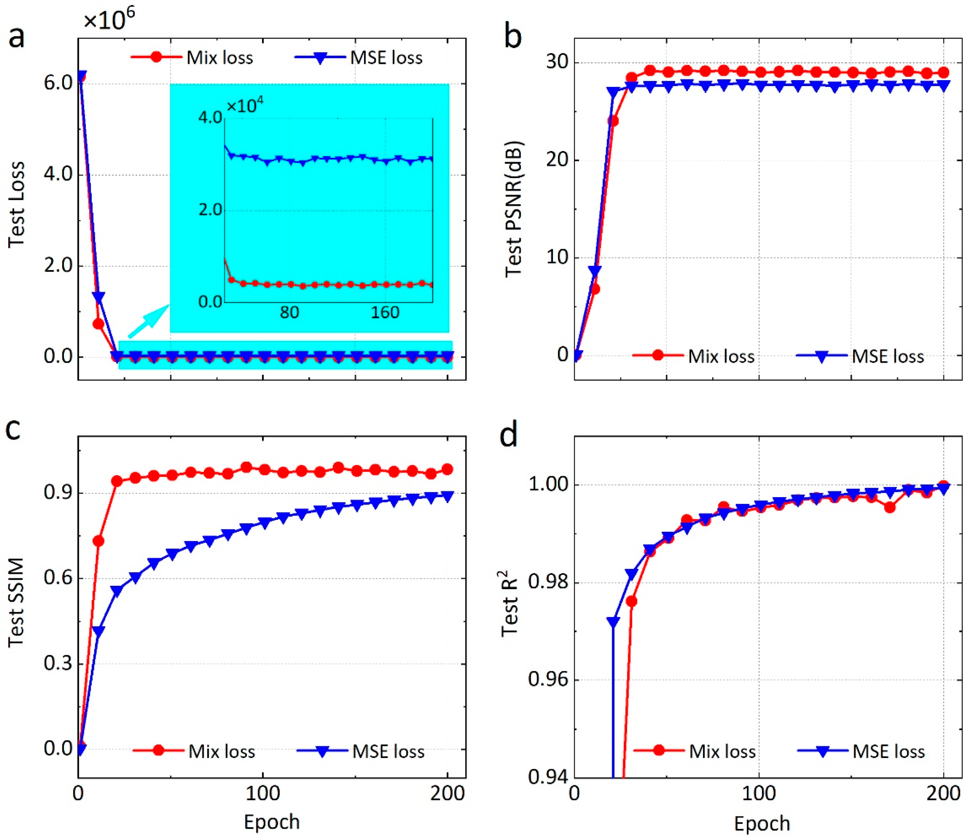
4.1. Optimized Performance of Loss Function

We first test the network optimization effect of the mix loss function from the synthetic dataset. Figure 5 exhibits the prediction results of AG-ResUnet trained with $L_{MSE}$ and $L_{Mix}$, respectively. Notice that ground truth is included as the reference. It is clear that the third row of estimated models by $L_{Mix}$ is close to the ground truth (Figure 5). For instance, the layered structure is clearly recovered in Figure 5b. Compared with $L_{MSE}$, inversion results of $L_{Mix}$ have more accurate salt dome boundaries (Figure 5). The inversion results of the $L_{Mix}$ are better than those of the $L_{MSE}$ in terms of SSIM, PSNR, and R².

The metrics relationships between the $L_{MSE}$ and $L_{Mix}$ for the test set are shown in Figure 6. When the epoch is less than 25, the PSNR and R² values of $L_{MSE}$ are slightly higher than those of $L_{Mix}$. As the training epoch increases, the test loss of $L_{Mix}$ converging is lower than that of $L_{MSE}$, and PSNR and SSIM are significantly higher than those of $L_{MSE}$. The R² values of the two loss functions show the same change trend, both close to 1. From the test set evaluation metrics (

Table 3. Performance metrics statistics and cost time of different loss functions on synthetic test set.

Dataset	Loss Function	Loss	PSNR	SSIM	R2	Time
Test	LMSE	29528.22	28.00	0.8636	0.9994	299 m 17 s
	LMix	3577.75	29.31	0.9903	0.9999	308 m 13 s

), the loss value of $L_{Mix}$ is an order of magnitude lower than that of $L_{MSE}$, while training times for both loss functions are almost the same. Tests based on synthetic data demonstrate that the $L_{Mix}$ improves the inversion accuracy without introducing extra computation. The $L_{Mix}$ is also used to train other networks in this study.

4.2. Qualitative Comparison

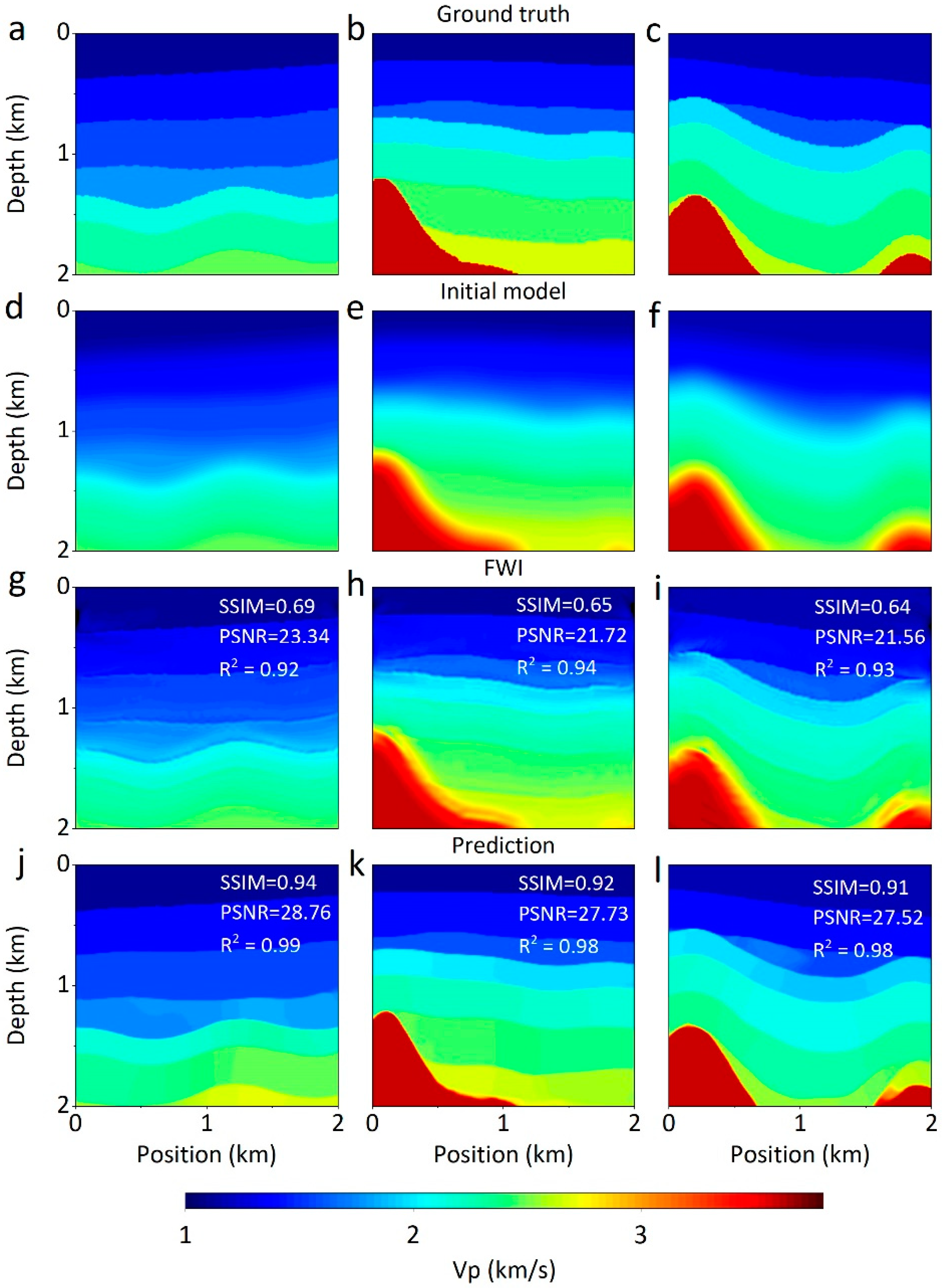
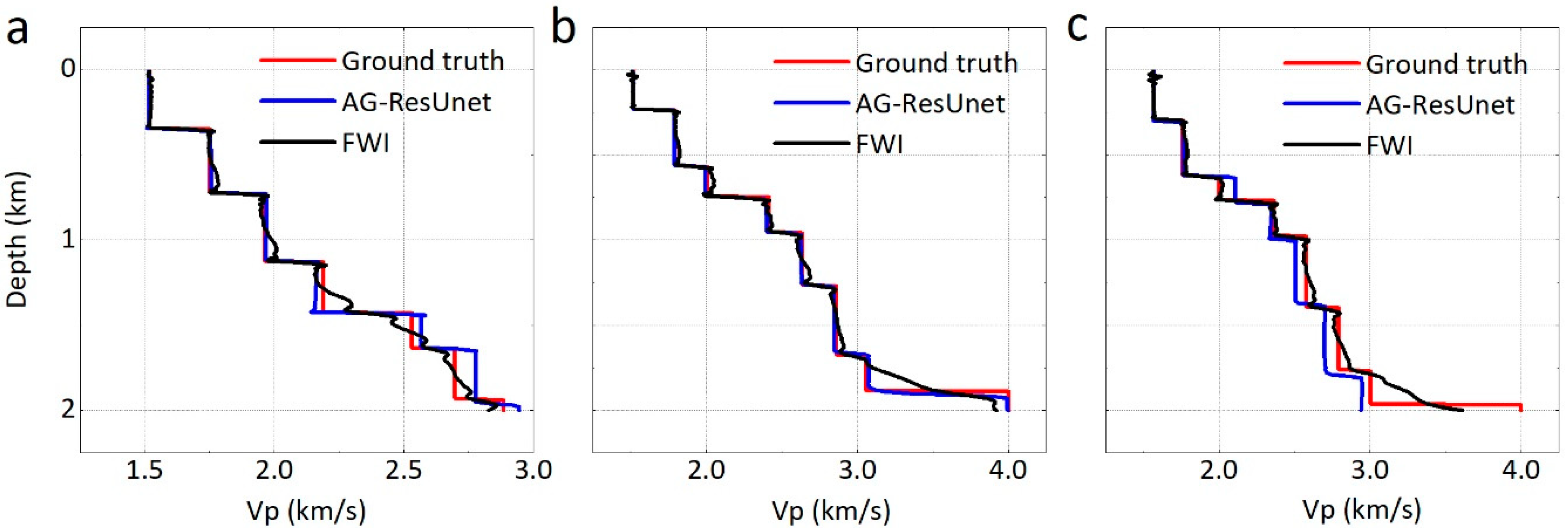
4.2.1. Comparison with Time-Domian FWI

Compared with AG-ResUnet and time-domain FWI, we analyzed performance between DL and the traditional inversion method. The forward parameters of FWI are assigned according to Table 1, and the conjugate gradient optimizer is employed. The inversion comparison based on the synthetic dataset is shown in Figure 7. Compared with the predictions and metrics of FWI, our approach has a more remarkable performance. The subsurface velocity models from AG-ResUnet (Figure 7j–l) are almost the same as the ground truth. Figure 7k,l can easily identify the salt dome outline. Although FWI can also retrieve the stratigraphic structure (Figure 7g–i), the resolution is low and structural boundaries are fuzzy.

To compare the efficiency of velocity inversion between FWI and AG-ResUnet, we illustrate the time consumed by FWI and AG-ResUnet for the training and inversion processes with the synthetic dataset (

Table 4. Time consumed of FWI and AG-ResUnet for the training and inversion processes in synthetic dataset. N/A indicates that FWI had no training time.

Dateset	Process	AG-ResUnet	FWI
Synthetic	Training	308 min 13 s	N/A
	Inversion	1.8 s	272 min 54 s

). Compared with FWI inversion time, the prediction time of the trained network is only 1.8 s, and the computational efficiency is much higher. To visualize the performance of our method, we plot the corresponding pseudo-logging data at the same position (Figure 8). It is clear that the velocity profiles of AG-ResUnet are nearly identical to the ground truth, but FWI velocity profiles exhibit slight fluctuations. What is more important is that AG-ResUnet is capable of precisely capturing the sudden velocity change (Figure 8).

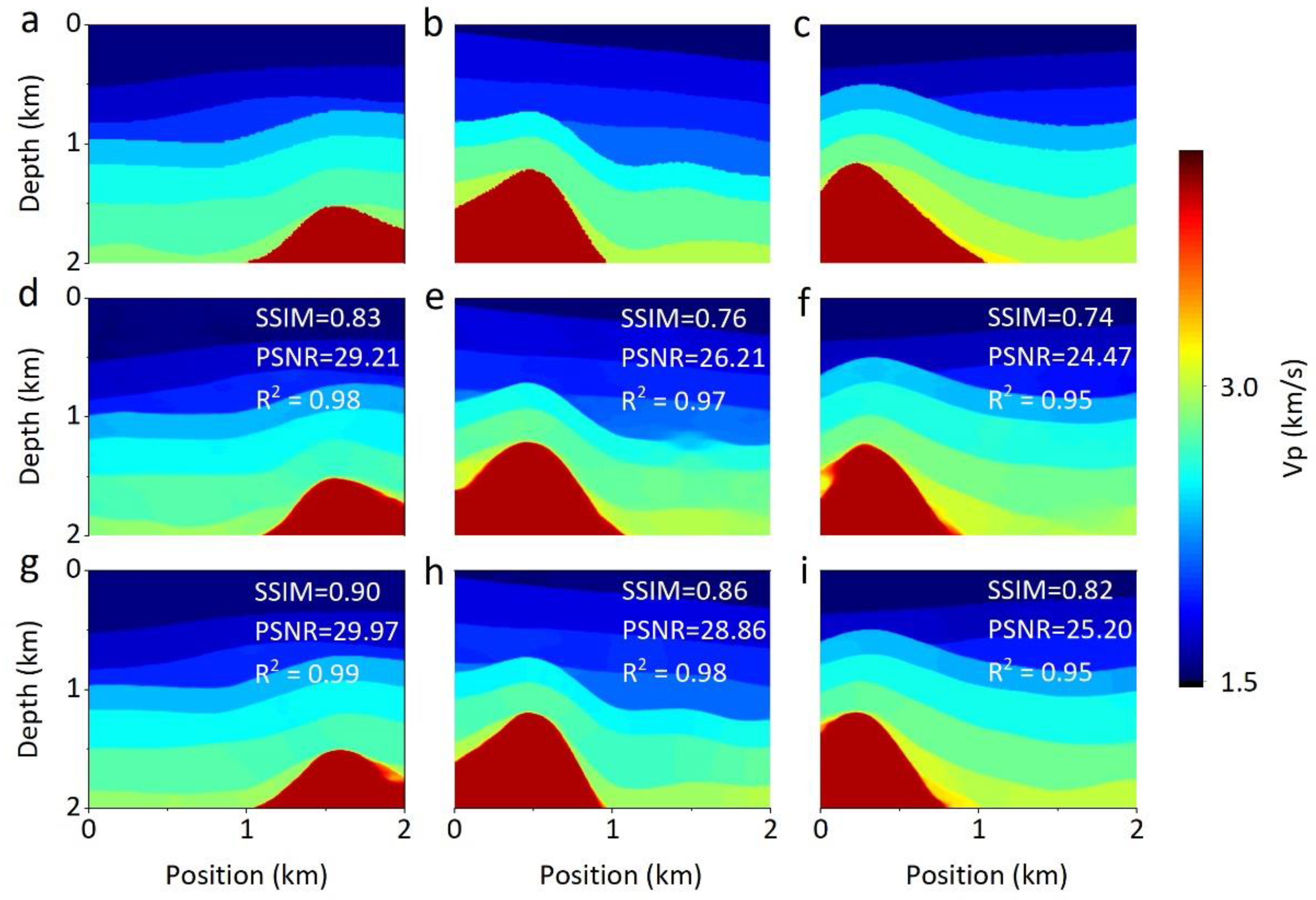
4.2.2. Comparison with Other Networks

To further demonstrate the superiority of AG-ResUnet for complex model inversion, we compared our approach with the other four DL algorithms, i.e., Unet, ResUnet, PSPnet, and DeepLab v3+, which have excellent ability in the segmentation field [65,66,67,68]. We apply the aforementioned network models to perform network training on synthetic datasets. We select predictions in the synthetic dataset to comprehensively compare the performance of algorithms (Figure 9). Generally, the results inverted by each network show relatively uniform and accurate velocity distribution. From the predictions and metrics, the velocity model predicted by AG-ResUnet is very close to the ground truth regarding the subsurface interface. Taking the salt dome structure as an example, AG-ResUnet successfully predicts the converging boundaries, while the predictions of other networks have significant errors.

In order to comprehensively compare the trend of the metrics during the training process of each network, we show the metrics history of five networks from the test set (Figure 10). The metrics of each network share the same trend. The loss term decreases significantly within 25 epochs and then converges smoothly. Besides, AG-ResUnet has the lowest test loss, and PSNR and SSIM reached a high point. We summarize the performance metrics statistics and cost time of five networks with the synthetic test set (

Table 5. Performance metrics statistics and cost time of five networks on synthetic test set. The bold numbers in this table indicate excellent performance.

Dataset	Network	Loss	PSNR	SSIM	R2	Time
Test	Unet	7046.72	27.30	0.9265	0.9994	208 min 56 s
	ResUnet	6045.29	28.05	0.9490	0.9998	295 min 26 s
	PSPnet	13662.38	28.03	0.6249	0.9756	157 min 48 s
	Deeplab v3+	4290.33	28.76	0.9545	0.9996	247 min 38 s
	AG-ResUnet	3577.75	29.31	0.9903	0.9999	308 min 13 s

), indicating that AG-ResUnet is more capable of extracting boundary features than other methods. Although it has the longest training time, the time difference is within one order of magnitude, and performance is totally acceptable given the competing power. The inversion comparison of AG-ResUnet and ResUnet shows that the AG unit is of great importance for enhancing the capability of identifying the subsurface velocity boundaries.

4.3. Network Generalization

In order to demonstrate the generalization of our method, we perform the transfer learning process with the SEG dataset and present the prediction results in Figure 11. The transfer learning results have accurately reconstructed the SEG salt body and clear subsurface interface. The inversion results and evaluation metrics on the SEG dataset demonstrate that transfer learning contributes to improving the trained network to identify new geological features.

To further demonstrate the training effect of transfer learning on mini-batch datasets, we show the metrics trend for transfer learning from the SEG test set (Figure 12). The loss term decreases considerably within ten epochs and then converges gradually. Similarly, PSNR, SSIM, and R² rise substantially within ten epochs and stabilize around a high level. The training metrics of the mini-batch SEG dataset are close to the level of the synthetic dataset. In particular, PSNR is stable at around 31 dB, which has exceeded the training performance on the synthetic dataset. The results show that our method is generalizable, and the trained AG-ResUnet can be an initial model to predict other datasets.

4.4. Network Stability

To analyze the stability of AG-ResUnet, we conduct additional experiments using both synthetic and SEG datasets under more realistic conditions. When the synthetic dataset is contaminated with a certain level of noise, the majority of predictions from AG-ResUnet (Figure 13) are close to the ground truth. However, overall predictions are slightly lower than those of clean data. When the noise level is low (e.g., SNR = 20 dB), it is clear in Figure 13d–f that the stratigraphic interfaces and the salt domes of inversion are accurate, with almost no artifacts. With the increase of noise (e.g., SNR ≤ 10dB), the inversion results become poor, yet the velocity model can still be correctly recovered. Moreover, we use AG-ResUnet to invert the noise-contaminated SEG dataset, and the inversion results still show the aforementioned regularity (Figure 14). The results demonstrate that our method can yield a stable velocity model from noise-contaminated data.

5. Discussion

We have demonstrated that our method can produce reliable results. The outstanding performance of AG-ResUnet benefits from the attention structure (i.e., AG). As illustrated by the workflow of AG in Section 2, this module fully considers the feature structure (e.g., geological targets and stratigraphic boundaries) extracted from the feature maps of the downsampling and upsampling process. We serve the feature structure extracted by AG as the training constraints. Therefore, our algorithm maintains a high boundary processing ability when dealing with different feature data. More importantly, the gating signal for each skip connection aggregates information from multiple scales, as shown in Figure 1, which increases the resolution of the reconstructed model and achieves better performance. By taking advantage of AG, our method is more robust and sensitive in extracting structural boundary information indicated by the inversion results of AG-ResUnet and other methods (Figure 7, Figure 8 and Figure 9). Another reason for introducing AG into the network is that it is simple to calculate. Notice that the AG parameters can generally be updated by back-propagation without employing a sampling-based method used in the traditional attention mechanisms [69]. Comparing the quantitative metrics of ResUnet and AG-ResUnet in Table 5, it is clear that the training time remains the same after introducing AG. In other words, AGs can be easily integrated into traditional CNN architectures with minimal computational overhead, increasing the model sensitivity and accuracy for predicting velocity models.

Moreover, the characterization of structural details also depends on the loss function. The error sensitivity approach (e.g., MSE loss function, mean absolute error (MAE) loss function) computes the error between each pixel of the prediction and the ground truth, which is insufficient to extract relevant structural information between each element. Therefore, to further improve the resolution of inversion, we introduce the SSIM into the loss function, which has been widely used in geophysical research, e.g., seismic velocity inversion [56] and seismogram super-resolution reconstruction [70]. The SSIM term comprehensively evaluates the structural similarity of the retrieved model so that the network optimization focuses on structural information. The inversion comparison in Figure 5 and Figure 6 shows that the combination of MSE and SSIM terms contributes to estimating accurate velocity models and mitigating the problem of non-uniqueness in inversion.

By taking advantage of the aforementioned improvements, the transfer learning and stability experiment results demonstrate that AG-ResUnet has a strong generalization, robustness, and the potential of processing field data. Due to the difference in the geological structure of different areas, it is reasonable to apply transfer learning to field data processing [49,71,72]. Transfer learning, in which we use the previously trained network as an initial network for an updated velocity model due to the change in geological conditions, can reduce the training costs and be adapted to more general field conditions. Notice that transfer learning also requires sufficient data. However, field data are usually very limited, making it difficult for data-driven DL methods to work. Nowadays, the physics-guided networks, relying on prior physical information, show the potential to solve the velocity inversions in case of limited data [73,74,75]. Therefore, future work may pay more attention to using prior physical information to guide the optimization of the network.

6. Conclusions

This study proposes a novel and practical approach to directly estimate velocity models from seismic data using AG-ResUnet. We have demonstrated that our approach can produce a reliable result. Our method has two advantages in network architecture and loss function. The AG-ResUnet network introduces attention gates that can adaptively detect areas with significant velocity changes, equivalent to introducing additional structural constraints for processing. Furthermore, the mix loss function contributes to the inversion results approximating the ground truth. By taking advantage of these two improvements, our method enhances the ability of DL algorithms to characterize detailed structures and retrieve complex velocity models.

AG-ResUnet provides a reliable way to strengthen the complex structure extraction from CSP gathers, showing excellent transfer learning properties and strong generalization. Experimental results demonstrate that our approach yields a stable and robust estimation in the cases of noisy data. To summarize, AG-ResUnet has high accuracy, strong generalization, and robustness for velocity inversion. Our method contributes to imaging geologic reservoirs, CO₂ monitoring, and geotechnical engineering.

References

1. Pan, X.; Zhang, P.; Zhang, G.; Guo, Z.; Liu, J. Seismic characterization of fractured reservoirs with elastic impedance difference versus angle and azimuth: A low-frequency poroelasticity perspective. Geophysics 2021, 86, M123–M139. [Google Scholar] [CrossRef]
2. Pan, X.; Li, L.; Zhang, G. Multiscale frequency-domain seismic inversion for fracture weakness. J. Pet. Sci. Eng. 2020, 195, 107845. [Google Scholar] [CrossRef]
3. Pan, X.; Zhang, G.; Yin, X. Azimuthally anisotropic elastic impedance parameterisation and inversion for anisotropy in weakly orthorhombic media. Explor. Geophys. 2019, 50, 376–395. [Google Scholar] [CrossRef]
4. Pan, X.; Zhang, G. Bayesian seismic inversion for estimating fluid content and fracture parameters in a gas-saturated fractured porous reservoir. Sci. China Earth Sci. 2019, 62, 798–811. [Google Scholar] [CrossRef]
5. Nguyen, P.K.T.; Nam, M.J.; Park, C. A review on time-lapse seismic data processing and interpretation. Geosci. J. 2015, 19, 375–392. [Google Scholar] [CrossRef]
6. Yilmaz, Ö. Seismic Data Analysis: Processing, Inversion, and Interpretation of Seismic Data; Society of Exploration Geophysicists: Houston, TX, USA, 2001. [Google Scholar]
7. Russell, B.; Hampson, D. Comparison of poststack seismic inversion methods. In SEG Technical Program Expanded Abstracts 1991; Society of Exploration Geophysicists: Houston, TX, USA, 1991; pp. 876–878. [Google Scholar]
8. Garotta, R.; Michon, D. Continuous analysis of the velocity function and of the move out corrections. Geophys. Prospect. 1967, 15, 584. [Google Scholar] [CrossRef]
9. Al-Yahya, K. Velocity analysis by iterative profile migration. Geophysics 1989, 54, 718–729. [Google Scholar] [CrossRef]
10. Dines, K.A.; Lytle, R.J. Computerized geophysical tomography. Proc. IEEE 1979, 67, 1065–1073. [Google Scholar] [CrossRef]
11. Tarantola, A. Inversion of seismic reflection data in the acoustic approximation. Geophysics 1984, 49, 1259–1266. [Google Scholar] [CrossRef]
12. Biondi, B.; Almomin, A. Simultaneous inversion of full data bandwidth by tomographic full-waveform inversion. Geophysics 2014, 79, WA129–WA140. [Google Scholar] [CrossRef]
13. Wu, Z.; Alkhalifah, T. Simultaneous inversion of the background velocity and the perturbation in full-waveform inversion. Geophysics 2015, 80, R317–R329. [Google Scholar] [CrossRef] [Green Version]
14. Yang, W.; Wang, X.; Yong, X.; Chen, Q. The review of seismic Full waveform inversion method. Prog. Geophys. 2013, 28, 766–776. [Google Scholar] [CrossRef]
15. Virieux, J.; Operto, S. An overview of full-waveform inversion in exploration geophysics. Geophysics 2009, 74, WCC1–WCC26. [Google Scholar] [CrossRef]
16. Sun, M.; Jin, S. Multiparameter Elastic Full Waveform Inversion of Ocean Bottom Seismic Four-Component Data Based on A Modified Acoustic-Elastic Coupled Equation. Remote Sens. 2020, 12, 2816. [Google Scholar] [CrossRef]
17. Tarantola, A. Linearized inversion of seismic reflection data. Geophys. Prospect. 1984, 32, 998–1015. [Google Scholar] [CrossRef]
18. Sen, M.K.; Stoffa, P.L. Nonlinear one-dimensional seismic waveform inversion using simulated annealing. Geophysics 1991, 56, 1624–1638. [Google Scholar] [CrossRef]
19. Jin, S.; Madariaga, R. Background velocity inversion with a genetic algorithm. Geophys. Res. Lett. 1993, 20, 93–96. [Google Scholar] [CrossRef]
20. Jin, S.; Madariaga, R. Nonlinear velocity inversion by a two-step Monte Carlo method. Geophysics 1994, 59, 577–590. [Google Scholar] [CrossRef]
21. Pratt, R.G.; Shin, C.; Hick, G. Gauss–Newton and full Newton methods in frequency–space seismic waveform inversion. Geophys. J. Int. 1998, 133, 341–362. [Google Scholar] [CrossRef]
22. Zhang, Y.; Gao, F. Full waveform inversion based on reverse time propagation. In SEG Technical Program Expanded Abstracts 2008; Society of Exploration Geophysicists: Houston, TX, USA, 2008; pp. 1950–1955. [Google Scholar]
23. Xu, W.; Wang, T.; Cheng, J. Elastic model low-to intermediate-wavenumber inversion using reflection traveltime and waveform of multicomponent seismic dataElastic reflection inversion. Geophysics 2019, 84, R123–R137. [Google Scholar] [CrossRef]
24. Wang, T.; Cheng, J.; Geng, J. Reflection Full Waveform Inversion With Second-Order Optimization Using the Adjoint-State Method. J. Geophys. Res. Solid Earth 2021, 126, e2021JB022135. [Google Scholar] [CrossRef]
25. Sirgue, L.; Pratt, R.G. Efficient waveform inversion and imaging: A strategy for selecting temporal frequencies. Geophysics 2004, 69, 231–248. [Google Scholar] [CrossRef] [Green Version]
26. Ko, S.; Cho, H.; Min, D.J.; Shin, C.; Cha, Y.H. A comparative study of cascaded frequency-selection strategies for 2D frequency-domain acoustic waveform inversion. In Proceedings of the 2008 SEG Annual Meeting, Las Vegas, NV, USA, 9–14 November 2008. [Google Scholar]
27. Bunks, C.; Saleck, F.M.; Zaleski, S.; Chavent, G. Multiscale seismic waveform inversion. Geophysics 1995, 60, 1457–1473. [Google Scholar] [CrossRef]
28. Shin, C.; Ha, W. A comparison between the behavior of objective functions for waveform inversion in the frequency and Laplace domains. Geophysics 2008, 73, VE119–VE133. [Google Scholar] [CrossRef]
29. Chung, W.; Shin, C.; Pyun, S. 2D elastic waveform inversion in the Laplace domain. Bull. Seismol. Soc. Am. 2010, 100, 3239–3249. [Google Scholar] [CrossRef]
30. Ha, W.; Kang, S.-G.; Shin, C. 3D Laplace-domain waveform inversion using a low-frequency time-domain modeling algorithm. Geophysics 2015, 80, R1–R13. [Google Scholar] [CrossRef]
31. Shin, C.; Ha, W.; Kim, Y. Subsurface model estimation using Laplace-domain inversion methods. Lead. Edge 2013, 32, 1094–1099. [Google Scholar] [CrossRef]
32. LeCun, Y.; Bengio, Y.; Hinton, G. Deep learning. Nature 2015, 521, 436–444. [Google Scholar] [CrossRef]
33. Choy, C.B.; Xu, D.; Gwak, J.; Chen, K.; Savarese, S. 3d-r2n2: A unified approach for single and multi-view 3d object reconstruction. In Proceedings of the European Conference on Computer Vision, Amsterdam, The Netherlands, 11–14 October 2016; pp. 628–644. [Google Scholar]
34. Goodfellow, I.; Bengio, Y.; Courville, A. Deep Learning; MIT Press: Cambridge, MA, USA, 2016. [Google Scholar]
35. Jin, K.H.; McCann, M.T.; Froustey, E.; Unser, M. Deep convolutional neural network for inverse problems in imaging. IEEE Trans. Image. Process. 2017, 26, 4509–4522. [Google Scholar] [CrossRef] [Green Version]
36. Meng, F.; Fan, Q.; Li, Y. Self-Supervised Learning for Seismic Data Reconstruction and Denoising. IEEE Geosci. Remote Sens. Lett. 2021, 19, 1–5. [Google Scholar] [CrossRef]
37. Dong, X.; Li, Y. Denoising the optical fiber seismic data by using convolutional adversarial network based on loss balance. IEEE Trans. Geosci. Remote Sens. 2020, 59, 10544–10554. [Google Scholar] [CrossRef]
38. Zhong, T.; Cheng, M.; Dong, X.; Li, Y. Seismic random noise suppression by using adaptive fractal conservation law method based on stationarity testing. IEEE Trans. Geosci. Remote Sens. 2020, 59, 3588–3600. [Google Scholar] [CrossRef]
39. Wang, B.; Zhang, N.; Lu, W.; Wang, J. Deep-learning-based seismic data interpolation: A preliminary result. Geophysics 2019, 84, V11–V20. [Google Scholar] [CrossRef]
40. Ovcharenko, O.; Kazei, V.; Kalita, M.; Peter, D.; Alkhalifah, T. Deep learning for low-frequency extrapolation from multioffset seismic data. Geophysics 2019, 84, R989–R1001. [Google Scholar] [CrossRef] [Green Version]
41. Huang, H.; Wang, T.; Cheng, J.; Xiong, Y.; Wang, C.; Geng, J. Self-Supervised Deep Learning to Reconstruct Seismic Data With Consecutively Missing Traces. IEEE Trans. Geosci. Remote Sens. 2022, 60, 1–14. [Google Scholar] [CrossRef]
42. Pham, N.; Fomel, S.; Dunlap, D. Automatic channel detection using deep learning. Interpretation 2019, 7, SE43–SE50. [Google Scholar] [CrossRef]
43. Wu, X.; Liang, L.; Shi, Y.; Fomel, S. FaultSeg3D: Using synthetic data sets to train an end-to-end convolutional neural network for 3D seismic fault segmentation. Geophysics 2019, 84, IM35–IM45. [Google Scholar] [CrossRef]
44. Das, V.; Mukerji, T. Petrophysical properties prediction from prestack seismic data using convolutional neural networks. Geophysics 2020, 85, N41–N55. [Google Scholar] [CrossRef]
45. Lewis, W.; Vigh, D. Deep learning prior models from seismic images for full-waveform inversion. In SEG Technical Program Expanded Abstracts 2017; Society of Exploration Geophysicists: Houston, TX, USA, 2017; pp. 1512–1517. [Google Scholar]
46. Araya-Polo, M.; Jennings, J.; Adler, A.; Dahlke, T. Deep-learning tomography. Lead. Edge 2018, 37, 58–66. [Google Scholar] [CrossRef]
47. Mosser, L.; Kimman, W.; Dramsch, J.; Purves, S.; De la Fuente Briceño, A.; Ganssle, G. Rapid seismic domain transfer: Seismic velocity inversion and modeling using deep generative neural networks. In Proceedings of the 80th Eage Conference and Exhibition 2018, Copenhagen, Denmark, 11–14 June 2018; pp. 1–5. [Google Scholar]
48. Wu, B.; Meng, D.; Zhao, H. Semi-supervised learning for seismic impedance inversion using generative adversarial networks. Remote Sens. 2021, 13, 909. [Google Scholar] [CrossRef]
49. Yang, F.; Ma, J. Deep-learning inversion: A next-generation seismic velocity model building method. Geophysics 2019, 84, R583–R599. [Google Scholar] [CrossRef] [Green Version]
50. Takam Takougang, E.M.; Bouzidi, Y. Imaging high-resolution velocity and attenuation structures from walkaway vertical seismic profile data in a carbonate reservoir using visco-acoustic waveform inversion. Geophysics 2018, 83, B323–B337. [Google Scholar] [CrossRef]
51. De Landro, G.; Serlenga, V.; Russo, G.; Amoroso, O.; Festa, G.; Bruno, P.P.; Gresse, M.; Vandemeulebrouck, J.; Zollo, A. 3D ultra-high resolution seismic imaging of shallow Solfatara crater in Campi Flegrei (Italy): New insights on deep hydrothermal fluid circulation processes. Sci. Rep. 2017, 7, 3412. [Google Scholar] [CrossRef] [PubMed]
52. Li, S.; Liu, B.; Ren, Y.; Chen, Y.; Yang, S.; Wang, Y.; Jiang, P. Deep-Learning Inversion of Seismic Data. IEEE Trans. Geosci. Remote Sens. 2020, 58, 2135–2149. [Google Scholar] [CrossRef] [Green Version]
53. Liu, B.; Yang, S.; Ren, Y.; Xu, X.; Jiang, P.; Chen, Y. Deep-learning seismic full-waveform inversion for realistic structural models. Geophysics 2021, 86, R31–R44. [Google Scholar] [CrossRef]
54. Wang, Z.; Bovik, A.C.; Sheikh, H.R.; Simoncelli, E.P. Image quality assessment: From error visibility to structural similarity. IEEE Trans. Image Process. 2004, 13, 600–612. [Google Scholar] [CrossRef] [Green Version]
55. Wu, Y.; Lin, Y. InversionNet: An efficient and accurate data-driven full waveform inversion. IEEE Trans. Comput. Imaging 2019, 6, 419–433. [Google Scholar] [CrossRef]
56. Geng, Z.; Zhao, Z.; Shi, Y.; Wu, X.; Fomel, S.; Sen, M. Deep learning for velocity model building with common-image gather volumes. Geophys. J. Int. 2022, 228, 1054–1070. [Google Scholar] [CrossRef]
57. Araya-Polo, M.; Adler, A.; Farris, S.; Jennings, J. Fast and accurate seismic tomography via deep learning. In Deep Learning: Algorithms and Applications; Springer: Berlin/Heidelberg, Germany, 2020; pp. 129–156. [Google Scholar]
58. Ronneberger, O.; Fischer, P.; Brox, T. U-net: Convolutional networks for biomedical image segmentation. In Proceedings of the International Conference on Medical Image Computing and Computer-Assisted Intervention, Munich, Germany, 5–9 October 2015; pp. 234–241. [Google Scholar]
59. He, K.; Zhang, X.; Ren, S.; Sun, J. Deep residual learning for image recognition. In Proceedings of the IEEE Conference on Computer Vision and Pattern Recognition, Las Vegas, NV, USA, 27–30 June 2016; pp. 770–778. [Google Scholar]
60. Oktay, O.; Schlemper, J.; Folgoc, L.L.; Lee, M.; Heinrich, M.; Misawa, K.; Mori, K.; McDonagh, S.; Hammerla, N.Y.; Kainz, B. Attention u-net: Learning where to look for the pancreas. arXiv 2018, arXiv:1804.03999. [Google Scholar] [CrossRef]
61. Lecomte, J.; Campbell, E.; Letouzey, J. Building the SEG/EAEG overthrust velocity macro model. In Proceedings of the EAEG/SEG Summer Workshop-Construction of 3-D Macro Velocity-Depth Models, Noordwijkerhout, The Netherlands, 24–27 July 1994; p. cp-96-00024. [Google Scholar]
62. Wu, X.; Geng, Z.; Shi, Y.; Pham, N.; Fomel, S.; Caumon, G. Building realistic structure models to train convolutional neural networks for seismic structural interpretation. Geophysics 2020, 85, WA27–WA39. [Google Scholar] [CrossRef]
63. Ren, Y.; Nie, L.; Yang, S.; Jiang, P.; Chen, Y. Building complex seismic velocity models for deep learning inversion. IEEE Access 2021, 9, 63767–63778. [Google Scholar] [CrossRef]
64. Paszke, A.; Gross, S.; Massa, F.; Lerer, A.; Bradbury, J.; Chanan, G.; Killeen, T.; Lin, Z.; Gimelshein, N.; Antiga, L. Pytorch: An imperative style, high-performance deep learning library. In Proceedings of the Advances in Neural Information Processing Systems 32 (NeurIPS 2019), Vancouver, BC, Canada, 8–14 December 2019; Volume 32. [Google Scholar]
65. Qamar, S.; Jin, H.; Zheng, R.; Ahmad, P.; Usama, M. A variant form of 3D-UNet for infant brain segmentation. Future Gener. Comput. Syst. 2020, 108, 613–623. [Google Scholar] [CrossRef]
66. Xiao, X.; Lian, S.; Luo, Z.; Li, S. Weighted res-unet for high-quality retina vessel segmentation. In Proceedings of the 2018 9th International Conference on Information Technology in Medicine and Education (ITME), Hangzhou, China, 19–21 October 2018; pp. 327–331. [Google Scholar]
67. Yan, L.; Liu, D.; Xiang, Q.; Luo, Y.; Wang, T.; Wu, D.; Chen, H.; Zhang, Y.; Li, Q. PSP net-based automatic segmentation network model for prostate magnetic resonance imaging. Comput. Methods Programs Biomed. 2021, 207, 106211. [Google Scholar] [CrossRef] [PubMed]
68. Wang, J.; Liu, X. Medical image recognition and segmentation of pathological slices of gastric cancer based on Deeplab v3+ neural network. Comput. Methods Programs Biomed. 2021, 207, 106210. [Google Scholar] [CrossRef]
69. Mnih, V.; Heess, N.; Graves, A. Recurrent models of visual attention. In Proceedings of the Advances in Neural Information Processing Systems 27 (NIPS 2014), Montreal, QC, Canada, 8–13 December 2014; Volume 27. [Google Scholar]
70. Li, J.; Wu, X.; Hu, Z. Deep learning for simultaneous seismic image super-resolution and denoising. IEEE Trans. Geosci. Remote Sens. 2021, 60, 1–11. [Google Scholar] [CrossRef]
71. Sun, J.; Innanen, K.A.; Huang, C. Physics-guided deep learning for seismic inversion with hybrid training and uncertainty analysis. Geophysics 2021, 86, R303–R317. [Google Scholar] [CrossRef]
72. Puzyrev, V. Deep learning electromagnetic inversion with convolutional neural networks. Geophys. J. Int. 2019, 218, 817–832. [Google Scholar] [CrossRef] [Green Version]
73. Sun, J.; Niu, Z.; Innanen, K.A.; Li, J.; Trad, D.O. A theory-guided deep-learning formulation and optimization of seismic waveform inversion. Geophysics 2020, 85, R87–R99. [Google Scholar] [CrossRef]
74. Alkhalifah, T.; Song, C.; bin Waheed, U.; Hao, Q. Wavefield solutions from machine learned functions constrained by the Helmholtz equation. Artif. Intell. Geosci. 2021, 2, 11–19. [Google Scholar] [CrossRef]
75. Rasht-Behesht, M.; Huber, C.; Shukla, K.; Karniadakis, G.E. Physics-Informed Neural Networks (PINNs) for Wave Propagation and Full Waveform Inversions. J. Geophys. Res. Solid Earth 2022, 127, e2021JB023120. [Google Scholar] [CrossRef]
Figure 1. A block diagram of AG-ResUnet network architecture. Each box represents the output feature maps of a convolutional layer. The number at the bottom of each box denotes channels in the corresponding feature map. The down-sampling module consists of the repeated two convolutional layers with 3 × 3 kernel sizes (blue arrow), two batch normalization layers (BN), linear rectification function (ReLU), and the 2 × 2 max-pooling layer (orange arrow). Each up-sampling module replaces the max-pooling layer with a 2 × 2 transposed convolutional layer (black arrow).
Remotesensing 14 03810 g001
Figure 2. Attention gate work flow [60] The two input signals x l and g l of AG from the down-sampled and corresponding up-sampled feature maps, respectively, x ^ is the feature map weighted by AG.
Remotesensing 14 03810 g002
Figure 3. The synthetic velocity models. (af) represent six representative velocity models from synthetic dataset. The red geological targets represent salt domes; other layered structures are surrounding formations.
Remotesensing 14 03810 g003
Figure 4. The SEG velocity models. (af) represent six representative velocity models from SEG dataset. The red geological targets represent salt, the blue represents background, and the white lines are stratigraphic boundaries.
Remotesensing 14 03810 g004
Figure 5. Predictions of networks trained with L M S E and L M i x in synthetic salt domes dataset. (ac) Ground truth, (df) LMSE results, and (gi) LMix results. The red geological targets represent salt domes, and other layered structures surround formations. The quantitative metrics in the inversion image are calculated from the inversion result and the corresponding ground truth; the metrics in the following inversion image are calculated this way.
Remotesensing 14 03810 g005
Figure 6. Comparison of quantitative metrics versus number of epoch between AG-ResUnet trained with L M S E and L M i x in synthetic salt domes dataset. (a) Test Loss, (b) test PSNR, (c) test SSIM, and (d) test R2. The red line represents the network’s performance trained by the mix loss function, and the blue line represents the MSE loss function training result.
Remotesensing 14 03810 g006
Figure 7. Comparisons of the velocity inversion in synthetic dataset. (ac) Ground truth, (df) initial velocity model of FWI, (gi) results of FWI, and (jl) predictions of our method. The initial model is the true velocity model after Gaussian smoothing with mean 0 and variance 8.
Remotesensing 14 03810 g007
Figure 8. Vertical velocity comparison. (ac) Pseudo-logging data of the ground truth (the models shown in Figure 7a–c) and corresponding predicted velocity at the position of 750 m. The red line represents the ground truth, the blue is the velocity variation of AG-ResUnet, and the black is FWI.
Remotesensing 14 03810 g008
Figure 9. Comparison of inversion results in different networks. (a) Ground truth, (b) Unet, (c) ResUnet, (d) PSPnet, (e) DeepLab v3+, and (f) AG-ResUnet. The metrics in each result show the inversion effect in terms of quantification.
Remotesensing 14 03810 g009
Figure 10. Quantitative metrics history of five networks trained in synthetic test dataset. (a) Test Loss, (b) test PSNR, (c) test SSIM, and (d) test R2.
Remotesensing 14 03810 g010
Figure 11. SEG salt body model inversion results. (ac) SEG models, (df) Salt body predictions by AG-ResUnet. The ground truth models are included as the reference.
Remotesensing 14 03810 g011
Figure 12. Quantitative metrics history of AG-ResUnet transfer learning in SEG test dataset. (a) Test Loss, (b) test PSNR, (c) test SSIM, and (d) test R2.
Remotesensing 14 03810 g012
Figure 13. Sensitivity of our method to noise in synthetic dataset. (ac) Ground truth, (df) predictions with 20 dB noisy seismic data, and (gi) predictions with 10 dB noisy seismic data.
Remotesensing 14 03810 g013
Figure 14. Sensitivity of our method to noise in SEG dataset. (ac) SEG models, (df) predictions with 20 dB noisy seismic data, and (gi) predictions with 10 dB noisy seismic data.
Remotesensing 14 03810 g014