Article

Elevation Change of CookE2 Subglacial Lake in East Antarctica Observed by DInSAR and Time-Segmented PSInSAR

Department of Geophysics, Kangwon National University, Chuncheon 24341, Korea
*
Author to whom correspondence should be addressed.
Remote Sens. 2022, 14(18), 4616; https://doi.org/10.3390/rs14184616
Submission received: 9 August 2022 / Revised: 5 September 2022 / Accepted: 13 September 2022 / Published: 15 September 2022
(This article belongs to the Special Issue Remote Sensing of Environmental Changes in Cold Regions Ⅱ)

Abstract

:
In this study, elevation change and surface morphology of CookE2, one of the most active subglacial lakes in East Antarctica, were analyzed by using Differential Interferometric Synthetic Aperture Radar (DInSAR) and a newly adapted Time-Segmented Persistent Scatterer Interferometric Synthetic Aperture Radar (TS-PSInSAR) techniques. Firstly, several DInSAR pairs were used to study the surface morphology of the subglacial lake during the rapid discharge event in 2007 and the subsequent recharge in 2010 by using ALOS PALSAR data and the continuous recharge from 2018 to 2020 by using Sentinel-1 SAR data. For time-series observation from 2018 to 2020, however, simple integration of DInSAR deviates largely from the satellite altimeter data because errors from the horizontal flow of the surrounding ice field or atmospheric phase accumulate. Conventional PSInSAR deviates from the altimeter data if the LOS displacement exceeds 300 mm, i.e., approximately 1/4 of the slant range resolution of the Sentinel-1 SAR in Interferometric Wide-swath (IW) mode, during the time window. Therefore, a series of Time-Segmented PSInSAR with a 4-month time window could accurately distinguish 1.10 ± 0.01 m/year of highly linear (R2 = 0.99) surface rise rate of CookE2 and 0.63 m/year of horizontal deformation rate of the surrounding ice field from 2018 to 2020.

Graphical Abstract

1. Introduction

Meltwater at the ice bed is an important component of the subglacial hydrologic system under the Antarctic ice sheet, which travels along the topography of the bedrock, creating channels and stored in watersheds to form subglacial lakes. The major source of meltwater at the ice bed of the Antarctic ice sheet is the liquid water produced by the pressure, insulation, and friction heat of thick ice [1]. The pressure caused by ice with a thickness of several thousand meters lowers the melting point of ice at the interface between the ice sheet and bedrock [2]. The presence of meltwater can accelerate the flow of glaciers by reducing friction between the ice and bedrock [3,4]. Bell et al. [5] suggested that large subglacial lakes can initiate rapid ice flow, which causes a change in the glacial mass balance. Therefore, it is important to observe the subglacial hydrologic system and the existence and deformation behavior of subglacial lakes.
The existence of most subglacial lakes has been confirmed by Radio Echo Sounding (RES), satellite altimeter, or seismic survey [1]. RES showed that the intensity of the reflected signal from the subglacial lake surface was much stronger and flatter than those from the bedrock due to the high contrast of dielectric constants between water and ice. Subglacial lake detection using a satellite altimeter can be performed by detecting the flat surface in a large subglacial lake or by detecting the change in altitude of the ice sheet above the active subglacial lake. Subglacial lakes have been studied intensively since Robin et al. [6] discovered “a thick water layer beneath the ice”. Ice-penetrating RES survey operated by the SPRI-TUD-NSF consortium (Scott Polar Research Institute, Technical University of Denmark, and National Science Foundation of the USA) from 1968 to 1979 has identified many subglacial lakes which were analyzed in the 1990s [7,8]. Since then, most subglacial lakes have been discovered using RES and satellite altimetry techniques [9,10,11]. Most subglacial lakes are reported to be ‘closed’ or ‘stable’ where inflows and outflows of the lake are nearly balanced so that no surface elevation change occurs. Some ‘active’ subglacial lakes have been identified where ice surface elevation changes [1]. Smith et al. [12] found a total of 124 active subglacial lakes in Antarctica using the Ice, Cloud, and land Elevation Satellite (ICESat) laser altimeter. The melt water below the ice sheet is driven by hydraulic pressure to discharge and recharge the subglacial lake, causing the upper ice sheet to fall or rise as the water level changes [13].
Since RES and satellite altimeters measure along the survey lines or satellite tracks, however, it is difficult to detect small subglacial lakes that lie between the lines. Performing airborne RES survey is time-consuming and can be constrained by weather and logistics, making it difficult to map entire Antarctica. Due to limitations in data acquisition, data coverage is often compensated by kriging interpolation [14]. Furthermore, the detection of a subglacial lake with the flatness of the ice surface would fail because the surface may appear smooth and flat with no relation to subglacial lakes. Moreover, the ice surface of subglacial lakes with less than 4 km in diameter may not be flat due to the thick ice cover [15]. The altitude accuracy of the altimeter is about 15 cm for ICESat, about 50 cm for CryoSat-2, and about 10 cm for ICESat-2 [16,17,18]. Active subglacial lakes can only be detected if there is an elevation change beyond these accuracies between the revisit cycle of the altimeter. As the revisit cycle is 369 days for CryoSat-2 and 91 days for ICESat-2, it might be difficult to detect episodic events that occur between revisit periods. More precise measurement with higher accuracy is necessary to monitor such rapid changes in subglacial lakes.
The satellite Synthetic Aperture Radar (SAR) is effective for research in Antarctica, where access is limited. It has the advantage of providing high-resolution images regardless of the illuminance of the sun and weather conditions. Differential Interferometric SAR (DInSAR) can be used to measure ice displacement in horizontal or vertical directions with centimeter accuracy. For example, Han and Lee et al. [19] calculated the exact horizontal flow velocity of the Campbell Glacier Tongue using the DInSAR technique and tidal correction. Since the DInSAR technique includes vertical displacement, changes in the elevation of the glacier surface can also be observed.
DInSAR is actively used to detect surface motion caused by volume changes in subglacial lakes. Gray et al. [20] used InSAR to observe changes in glacial surface elevation due to the movement of subglacial water. Capps et al. [21] used European Remote-sensing Satellite-1/-2 (ERS-1/-2) tandem data to determine the displacement and volume of subglacial lakes located on the Brady Glacier in Alaska. Palmer et al. [22] determined glacial subsidence due to drainage of a subglacial lake, considering that displacement using InSAR is in the Line-Of-Sight (LOS) direction. Neckel et al. [23] analyzed the movement occurring in the hydrologically connected subglacial lakes through Sentinel-1 DInSAR images.
Double-Differential Interferometric SAR (DDInSAR) is a technique that can calculate the amount of displacement change obtained from the DInSAR pair. It is possible to remove the same components from two DInSAR images and extract only the parts that have changed. For example, Lee et al. [24] found the accelerating motion of subglacial lakes in Campbell Glacier using DDInSAR. Elevation change due to subglacial lakes was calculated using the DDInSAR technique to cancel constant surface ice flow.
A recently developed variant of the InSAR technique, Persistent Scatterer Interferometric SAR (PSInSAR), facilitates time-series analysis using many interferograms. Stable scatterers are selected to calculate the surface displacement over time to monitor surface changes such as subsidence, volcanic activity, and landslides [25,26]. In Antarctica, PSInSAR has a lot of potential but has not been fully exploited, except for the research of Pandit et al. [27] that used it to calculate the ice flow velocity.
Among over 140 active subglacial lakes found in Antarctica so far, CookE2, located in East Antarctica, attracted the attention of many researchers due to its rapid drainage between 2006 and 2008. Previous studies confirmed vertical subsidence of 70 m using ICESat data [9,12,28,29]. Using various data based on altimeter or optical satellites, they analyzed the surface elevation change due to recent recharging [9,28,29]. Most of the previous studies focused on the area, volume changes, and the rate of surface elevation change of the subglacial lake using altimeter and optical data, and few have used SAR data so far. In this study, we propose the application of various InSAR techniques to the observation of subglacial lakes in Antarctica with higher spatial and temporal accuracy. Surface morphology during the rapid discharge of CookE2 in 2007 and 2009 will be observed by using DInSAR, while a modified PSInSAR will be used to observe the time-series motion of subglacial lakes during the recent recharge of the lake.

2. Materials

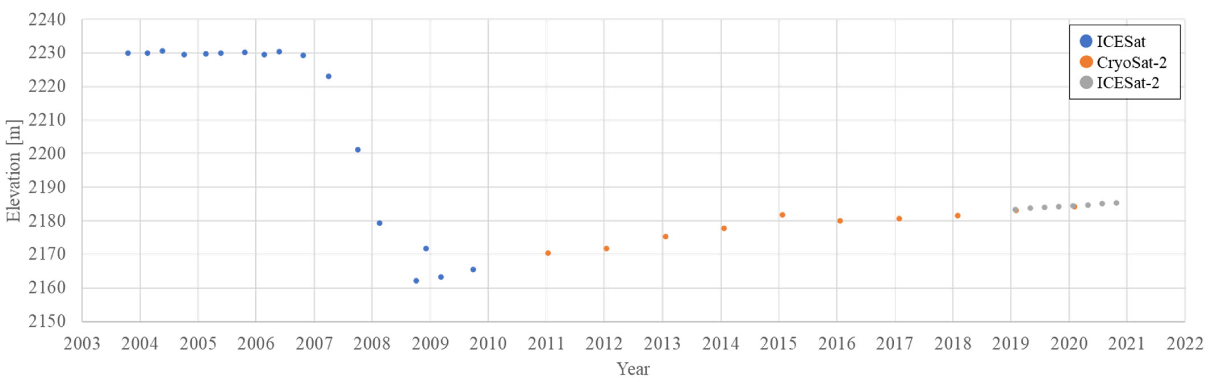
2.1. Study Area and Satellite Altimeter Data

The study area is CookE2 subglacial lake, located upstream of Cook Basin (Figure 1). The area observed in this study is approximately 100 km west of Talos Dome and about 20 km from the ice divide. The horizontal ice flow over CookE2 is relatively slow because it is located close to the ice divide where the flow begins. Ice flow velocity calculated from data obtained through NASA Making Earth System Data Records for Use in Research Environments (MEaSUREs) Program is approximately 0.6 m/year [30,31].
Lake CookE2 was first listed on the inventory of active subglacial lakes by Smith et al. [12], who reported that 2.7 km3 of water was drained from CookE2 from November 2006 to March 2008 by using ICESat laser altimeter data. A 44 m decrease in surface height was observed in track 227 of ICESat, and a 48 m decrease in track 1325, which is approximately five times the height decrease found in other subglacial lakes by that time. McMillan et al. [9] combined ICESat and CryoSat-2 data to construct a time series of the surface elevation and observed that the surface height of the CookE2 decreased sharply from 2006 to 2008 at an average rate of 35 ± 14 m/year and then increased again to 5.6 ± 2.8 m/year. The uncertainty of the discharge rate (14 m/year) was high because they assumed that the discharge rate was constant over time, which is shown in Figure 2, and it was not sure when the drainage was completed at that time. They estimated the surface depression area of CookE2 to be 260 m2 through ice surface mapping using CryoSat-2. Flament et al. [28] observed an elevation decrease of about 70 m from November 2006 to October 2008 through ICESat. They reported an elevation increase of about 13 m between October 2008 and February 2012 by using ICESat and the SPOT5 Digital Elevation Model (DEM). They derived the total discharge from elevation change and lake area to be 5.16 ± 1.52 km3. Additionally, observations of elevation changes between September 2002 and October 2010 based on Envisat radar altimeter (RA-2) data showed that the drained subglacial water was not completely discharged into the sea. Li et al. [29] showed a decrease in elevation of 59.6 m from February 2006 to October 2008 due to drainage, followed by a steady increase at a rate of about 1.1 m/year from January 2011 to November 2016 using ICESat and CryoSat-2 data. They used airborne ice-penetrating radar data to redefine the lake area to be the area where water exists. The result of Li et al. [29] was evaluated to be narrow compared to other studies. Results from 4 studies on CookE2 are summarized in Table 1. CookE2 is always listed as an active subglacial lake in the recently published global inventory of subglacial lakes [1,33].
Most of the researchers performed their observations using ICESat and CryoSat-2 altimeters. All altimeter data at the center of CookE2 is shown in Figure 2, including recent ICESat-2 data. ICESat data were acquired from Campaign 2A to Campaign 2F from 2003 to 2009 and represent the maximum surface subsidence point values for each acquisition time. However, due to the orbital repeatability error and the slight sampling shift of ICESat, each value was not obtained at the same point. This can result in differences of up to 0.5 km from the collection location, but another reason can lead to larger errors. Specifically, data were acquired from tracks 227 and 1325. Because the data acquisition directions of the two tracks are different and intersect, the sampling points on each track are up to 2 km apart. CryoSat-2 data were acquired using level 2 products acquired in SARIn mode. A total of 10 data were acquired at an interval of 369 days from 19 January 2011 to 15 February 2020. In this study, ICESat-2 data were additionally obtained from 11 February 2019 to 9 November 2020 on track 965 across CookE2 every 91 days [34].

2.2. Synthetic Aperture Radar (SAR) Data

The main purpose of this study is to observe the CookE2 subglacial lake and its discharge and recharge events from 2007 by using satellite SAR images. In previous studies, satellite altimeters were mainly used along the satellite tracks. However, satellite SAR imagery allows the identification of two-dimensional structures by using amplitude images and interferometric capabilities. In addition, the satellite SAR system has a shorter repetition cycle than that of satellite altimeters, which can improve the data acquisition frequency significantly. In this study, a total of 116 SAR images acquired from two SAR platforms from 2007 to 2020 were used (Table 2).
Advanced Land Observing Satellite (ALOS) Phased Array L-Band Synthetic Aperture Radar (PALSAR), operated by the Japan Aerospace Exploration Agency (JAXA) was launched in 2006 and operated until 2011 [35,36]. PALSAR, one of the three sensors installed in ALOS, has an L-band (1.27 GHz) SAR system and operates in fine mode, scan SAR mode, and polarimetric mode [37]. In this study, SAR images acquired in Fine Beam Single polarization (FBS) mode were obtained in level 1.1 Single Look Complex (SLC) products. Two interferometric pairs in 2007 and 2010 were available from the ALOS archive products.
The Sentinel-1 satellites, operated by the European Space Agency (ESA), are composed of dual Sentinel-1A and Sentinel-1B satellites launched in 2014 and 2016, respectively [38]. Each satellite acquires data of the same ground area every 12 days using the C-band (5.405 GHz) SAR system, but data could also be acquired every 6 days because both satellites share the same orbit plane [39]. However, recently, it has been known that Sentinel-1B does not transmit data due to a power system issue, and since 23 December 2021, data are acquired every 12 days using only the Sentinel-1A satellite [40]. We used 112 data acquired every 6 or 12 days from 12 September 2018 to 30 December 2020. Each SAR data are provided as an SLC product obtained in Interferometric Wide-swath (IW) mode.

3. Methods

3.1. Differential Interferometric SAR (DInSAR)

Using the interferometric phase of two SAR images acquired from repeated orbits of a satellite SAR system, it is possible to detect a subtle change of position of the ground target over time. The interferogram shows fringes that include both the phase by topographical elevation and the phase by ground displacement. In order to observe only the displacement of the surface, it is necessary to remove the phase by topographical elevation. Therefore, the DInSAR technique using a reference DEM was applied to remove the topographic phase. Coherence images obtained during the DInSAR processing were analyzed to confirm the surface stability and morphology. The coherence image provides information about the consistency between the InSAR pair [41]. When temporal or spatial decorrelation occurs between two images, the coherence has a low value close to 0, and a high value close to 1 when there is no change. In this study, the shape of the surface of the subglacial lake was analyzed using InSAR coherence images as well as interferograms.
DInSAR processing was performed on ALOS PALSAR images and Sentinel-1 SAR images using SeNtinel Application Platform (SNAP) software. For ALOS PALSAR images, we first co-registered two level 1.1 products, and a deskewing operator was used to perform the necessary geometric corrections. During the interferogram generation, the flat earth phase and the topographic phase were subtracted, and the coherence was estimated as well. The Copernicus 30 m Global DEM was used to calculate the topographic phase. Goldstein phase filtering was applied to enhance the signal-to-noise ratio of the final ALOS DInSAR image [42]. For the Sentinel-1 DInSAR pairs, adequate sub-swath and bursts of the study area were selected in the TOPSAR split operator of the SNAP, and then Sentinel Precise orbital state vector was applied. Interferograms with neighboring SAR acquisition dates were generated by co-registering with the Sentinel-1 back geocoding operator, and the burst overlaps were removed with the TOPSAR deburst operator. In the same way as in the ALOS PALSAR process, flat earth phase removal, topographic phase removal using Copernicus 30 m Global DEM, and coherence estimation were performed during the interferogram generation. Finally, the Sentinel-1 DInSAR result image was obtained by removing phase noise through Goldstein phase filtering [42]. Note that one fringe in the DInSAR image means a displacement of half the wavelength in the LOS direction.
Lee and Seo [43] estimated the vertical displacement of the subglacial lake based on Sentinel-1 SAR data from October 2018 to June 2019. The vertical displacement measured in meters per 12 days was extracted at the center of CookE2, as plotted in blue dots in Figure 3. The data are then integrated to be compared with the ICESat-2 altimeter data (yellow dots in Figure 3). The linear regression of the DInSAR results shows that uplift occurred at a rate of about 1.61 m/year, while the ICESat-2 observation is about 1.17 m/year. The difference is probably because the DInSAR signal contains not only the vertical motion of CookE2 but also the horizontal ice flow and atmospheric effect. The atmospheric effect may cancel out during the integration of DInSAR time series data as it is basically a random process. However, the signal from the horizontal ice flow of the CookE2 and the surrounding ice field will be deterministic and linear, which will be accumulated during the integration of the DInSAR signal.
Figure 4 shows an example of the Sentinel-1 DInSAR images. A linear phase trend appeared around the CookE2 subglacial lake, making it difficult to accurately separate it from the vertical motion. This linear phase could be either from atmospheric noise or strains due to the horizontal ice flow of this region. Anyway, this linear phase can be calculated (Figure 4b) and eliminated (Figure 4c) for each DInSAR image. Reprocessing individual DInSAR images in this way is inconvenient and inadequate, which raised the necessity of introducing a more sophisticated time-series analysis such as PSInSAR.
It is worth paying attention to the uncertainty in setting the zero-displacement point when analyzing displacement over time. For example, in Figure 4c, a difference in the number of fringes occurs when a point with green close to yellow is selected as a zero-displacement point and when a point with green close to blue is selected. As a result, an error can occur, and the accumulation of errors in time series analysis can lead to larger differences. Therefore, the DInSAR technique may obtain displacements during the acquisition period of a DInSAR pair but may not be suitable for time series analysis as there is a risk of error accumulation.
The DDInSAR technique is another option, as it is widely used to observe surface motion over subglacial lakes [24,44,45]. However, subglacial lakes must have an acceleration of motion to be found by the DDInSAR technique. Because DDInSAR can eliminate constant deformation rates between two DInSAR observations, it is easy to find subglacial lakes that change seasonally or cyclically. However, it is difficult to apply the DDInSAR technique in this study area because both the horizontal flow rate and the vertical displacement of CookE2 are almost constant during the recharge period after 2009. Therefore, both phases from ice flow and surface rise will be removed during the DDInSAR operation, as shown in Figure 5.
In conclusion, DInSAR interferogram and coherence imagery gives valuable information on surface deformation and morphology but may not be efficient for time-series analysis of the surface motion due to errors from atmospheric phase and horizontal ice flow. More sophisticated algorithms for the time-series InSAR technique are considered, as described in the next section.

3.2. Time-Segmented Persistent Scatterer InSAR (TS-PSInSAR)

Since it was confirmed that simply integrating the DInSAR results is not suitable for time series analysis of the study area, we tried to measure the displacement over time by applying the PSInSAR technique that uses highly consistent Persistent Scatterers (PS) [25]. We used the Stanford Method for Persistent Scatterers (StaMPS) package [46]. PSs were selected considering the spatiotemporal consistency of SAR amplitudes and phase of the interferograms. The phase of PSs is then statistically analyzed to estimate displacement and various errors. Firstly, SNAP software was used as a pre-processing tool to generate time-series interferograms and other datasets for the input of the StaMPS package. Several key parameters changed from the default value of StaMPS have been summarized in Table 3.
Figure 6 is the result of the orbital ramp phase removal tool estimated during the StaMPS processing for 4 months with a master date of 6 November 2020. This function estimates the linear phase trend over the whole image, assuming that the orbital error is highly linear in each DInSAR. Figure 6a indicates the estimated phase is highly cumulative in time from the master image of 6 November 2020, which is obviously not the case of the orbital ramp that should be in a random fashion. The estimated linear phase trend is similar to the linear phase of the DInSAR image due to the horizontal ice flow of the study area. Using the orbital ramp phase estimation function of StaMPS, it would be more convenient to remove the linear phase caused by the horizontal ice flow than to remove them one by one from each DInSAR image.
The linear phase in Figure 6a has a maximum phase change of about 30 radians for two months. Based on this, the displacement R in the range direction (LOS direction) can be obtained using the following equation:
ϕ = 4 π λ R ,
where ϕ is the phase change and λ is the wavelength of the SAR system. The horizontal displacement in the range direction can be expressed as follows because movement by the flow is projected in the LOS direction:
R = f · l ^ = f f ^ · l ^ .
Here, the unit vector for the LOS direction l ^ and the unit vector for the flow direction f ^ are known values and we want to know the magnitude of the horizontal deformation by flow |f|. Substituting Equation (2) into Equation (1) gives:
ϕ = 4 π λ f f ^ · l ^ .
replacing Equation (3) for f , we obtain:
f = λ 4 π ϕ 1 f ^ · l ^ .
|f| is calculated to be 26 cm for two months in this study, which corresponds to a horizontal deformation rate of about 1.53 m/year across the image, as shown in Figure 6. Dividing this number by 29 km, the length of the whole region, gives the strain rate of 5 .276 × 10 5   year 1 . Multiplying it with 12 km, the size of the lake, including the hook-shaped zone, gives the horizontal deformation rate across the lake to be 0.63 m/year. If this horizontal deformation rate is misinterpreted as a vertical displacement in DInSAR, it gives an error of 0.42 m/year. This error is similar to the one in Figure 3, which shows the over-estimation of the uplift rate by 0.44 m/year obtained from cumulative DInSAR (1.61 m/year) when compared with that of the altimeter (1.17 m/year) if not compensated properly.
Because the downstream of the ice sheet flows relatively faster than the upstream, the deformation is thought to have caused the phase of a linear trend, as shown in Figure 6a. If this phase is not sufficiently removed, a larger value is derived when calculating the rate of surface rise. Therefore, we concluded that the application of the PSInSAR technique, which can automatically eliminate these errors, could yield better results.
Before the above 4-month PSInSAR experiment, our initial attempt of PSInSAR with the whole 112 Sentinel-1 SAR data obtained for 28 consecutive months from September 2018 to December 2020 failed. There were no sufficient PSs that survived during the PSInSAR processing over the entire period because of the continuous flow of glaciers in one direction and the rapid rise of the subglacial lake, as well as suffering from temporal decorrelation. Therefore, data for the last 10 months in 2020 have been processed on a trial basis with a reduced period (black lines and black dots as a master image in Figure 7). As a result, the center of the subglacial lake showed unexpected results compared to other relatively stable areas outside, showing a relatively slower rate initially and then accelerated to show a linear trend after 5 months (Figure 8a and Figure 9). Such a trend in elevation changes was not observed in the altimeter data, which showed linear uplift during this period (Figure 2 and Figure 3). This is because the deformation at the center of the subglacial lake is much faster than those of other geophysical phenomena in previous PSInSAR studies. Therefore, the fewer number of PSs remains over a long period because the surface scatterers move continuously, and PSs are affected by the adjacent pixels. Therefore, special care must be taken to ensure that the displacement does not exceed some fraction of the range resolution of the SAR image during the PSInSAR dataset period. Otherwise, an error could occur near the early and later stages of the observation period due to interference with the neighboring PS pixels.
To overcome the data duration issue for PSInSAR for fast-moving ice surfaces, we decided to separate the duration of data for each PSInSAR into 4-month (red and blue lines and dots in Figure 7 and Figure 8b,c). At the center of the subglacial lake (A points), the result was linear, similar to the rate of the later stage (Figure 9a). No significant errors were found in the displacements of subglacial lake edges (B points) or hook-shaped zone (C points) (Figure 9b,c), or even at the point where no displacement is expected (D points) (Figure 9d).
Figure 9a suggests that two Time-Segmented PSInSAR results within 4 months produce liner trends successfully with a maximum displacement of 300 mm at the center of CookE2. Considering the slant range resolution of 2.4 m of Sentinel-1 SAR, the 300 mm of displacement corresponds to 1/8 of the slant range resolution, which is within a general requirement of accuracy for conventional InSAR coregistration. Considering the recent surface uplift rate of about 1.17 m/year confirmed by the altimeter data at the center of CookE2 and the local incidence angle of 33.65 degrees, the LOS displacement rate is calculated to be 0.974 m/year.
Therefore, a total of 28 months of data were time-segmented at 4-month intervals and processed for PSInSAR so that 7 segments cover the whole period. SAR data overlapped between the segments to connect them. We named this technique as Time-Segmented PSInSAR (TS-PSInSAR), stating that the data duration for PSInSAR should be segmented in time and later linked by the overlapping dates so that the maximum LOS displacement during each segment should be within 1/8 of the slant range resolution. An in-depth analysis of the TS-PSInSAR results, such as how similar these results are to altimeter data in practice, will be discussed in the next section.

4. Results

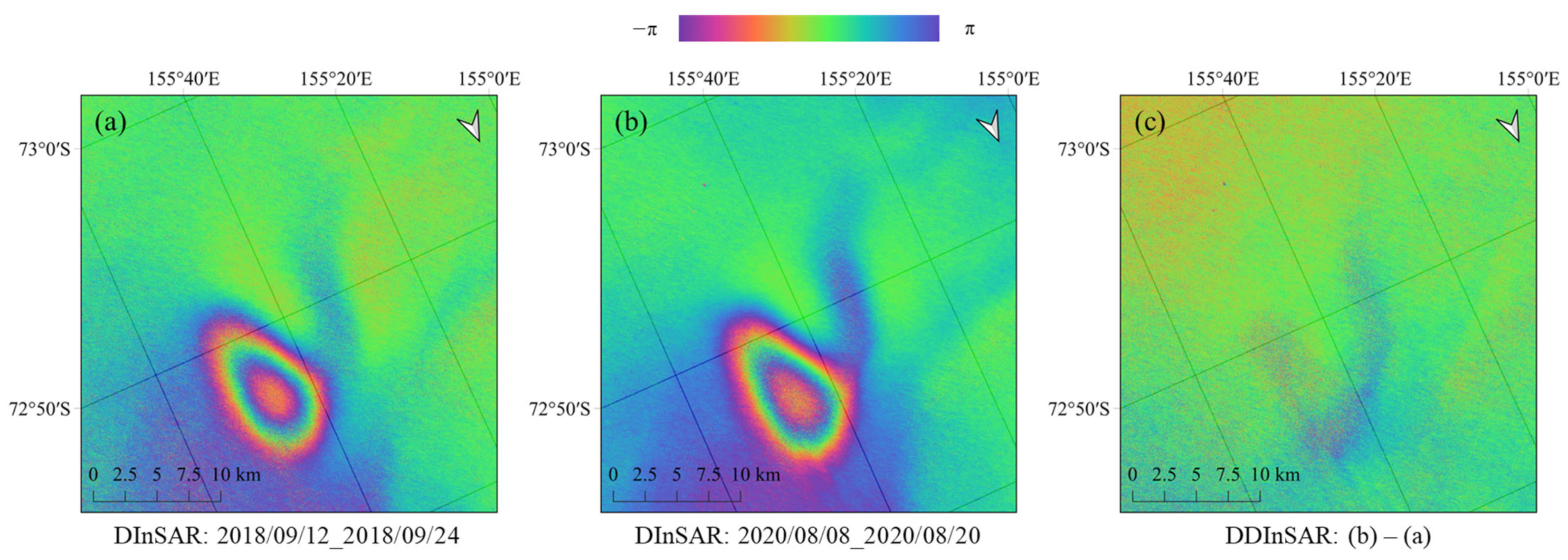
4.1. Surface Morphology of CookE2 during Discharge and Recharge Observed by DInSAR

Using DInSAR interferograms and coherence images, surface displacement and morphology were investigated during the discharge and recharge of the CookE2 subglacial lake (Figure 10). Analyze displacements in order of time and then identify morphological features.
According to ICESat laser altimeter data referenced in previous studies, episodic discharges in Lake CooKE2 from November 2006 to October 2008 resulted in a surface elevation change of approximately 67.11 ± 0.15 m [9,12,28,29]. However, those altimetry results were along the satellite tracks only, and the whole displacement field of the subglacial lake was hardly observed. In this study, displacements from 15 November 2007 to 31 December 2007 were analyzed using an ALOS DInSAR image (Figure 10a). The concentric fringes show the LOS displacement according to the volume change of the subglacial lake. A large number of fringes appeared not only on the main lake but also on the hook-shaped zone on the upper-right side. The hook-shaped zone appears over a large area, of which the length is approximately equal to the length of the main lake. About 51.7 fringes were identified on the main lake, and 16.5 fringes were found on the hook-shaped zone. Considering the wavelength of 23.6 cm for ALOS PALSAR, they correspond to 6.10 ± 0.12 m and 1.95 ± 0.12 m subsidence in the LOS direction in 46 days, respectively. Here we put the uncertainty of phase measurement of one fringe due to the displacement (half the wavelength) of the surrounding ice field. Assuming that vertical subsidence due to the drainage of subglacial lakes is dominant, those LOS displacements can be converted to the vertical subsidence of 8.00 ± 0.15 m on the main lake and 2.54 ± 0.15 m on the hook-shaped zone in 46 days. Verification was attempted by comparing this result with the displacement confirmed in the ICESat data, which shows the subsidence of 21.90 ± 0.15 m between 5 October 2007, and 20 February 2008 (Figure 2). Assuming that the rate of subsidence is linear during this period, altimeter data show that there was a subsidence of about 7.30 ± 0.15 m over 46 days, which is similar to the DInSAR result above. Minor differences may have come from the offset between the maximum displacement point of the altimeter track and that of DInSAR.
According to the previous studies and the altimeter data in Figure 2, the altitude of the CookE2 has increased steadily since it reached its lowest value in October 2008. It was estimated that the surface has been rising again due to the recharging at CookE2 after the drainage was completed. We analyzed an ALOS DInSAR pair to measure the surface displacement in 2010 when all altimeter data collection was temporarily stopped (Figure 10b). Between 20 October 2010, and 5 December 2010, ALOS DInSAR confirmed that the number of fringes of the main lake reduced significantly, and there was almost no displacement on the hook-shaped zone. It is estimated that the recharging of the lake started before 2010, and it can be expected that there was little change on the surface because the hook-shaped zone was not sufficiently filled with water. Three fringes can be identified on the main lake, which corresponds to 0.35 ± 0.12 m in the LOS direction and 0.46 ± 0.15 m vertical uplift in 46 days. Flament et al. [28] calculated the displacement for the period including 2010 using ICESat data measured on 12 March 2009 and SPOT5 data observed on 9 February 2012. An increase of about 10–15 m has been reported over 1064 days, which corresponds to 0.46–0.65 m vertical uplift in 46 days.
Figure 10c is a Sentinel-1 DInSAR image showing the displacement between 8 August 2020 and 20 August 2020. Sentinel-1 uses a C-band SAR system of which the wavelength system is 5.6 cm. One fringe of the DInSAR interferogram represents a LOS displacement of half the wavelength, i.e., 2.8 cm. About 1.3 fringes appeared in the main lake, which corresponds to 3.6 ± 0.7 cm in the LOS direction in 12 days. Here we found the uncertainty of fringe measurement of about 1/4 fringe (1/8 wavelength) originating from the remnant fringes surrounding the lake. This value can be interpreted as a 4.4 ± 0.8 cm uplift in 12 days. During the study period using Sentinel-1 SAR DInSAR images, the surface elevation increased at a rate of 3–6 cm in 12 days and showed a continuous uplift trend. However, a weak or no displacement signal was observed over the hook-shaped zone in the Sentinel-1 DInSAR images.
In 2007 when a massive discharge of the subglacial lake occurred, the deformation over a hook-shaped zone appeared much wider than reported in Smith et al. [12], but from 2010, it became much smaller. It is necessary to explain why the elevation changed at a different rate. A ridge area was identified between the main lake and the hook-shaped zone by using the Multichannel Coherent Radar Depth Sounder 5 (MCoRDS5) airborne radar data, which is a multi-channel radar operated by the Center for Remote Sensing of Ice Sheets (CReSIS) and is used to observe the ice sheet thickness and ice bottom [48]. (Figure 11). Ice bottoms were identified using L1B and L2 datasets with segment ID 04 and frame number 010 acquired on 29 November 2017 during an IceBridge mission [49,50]. The ridge point between the main lake and the hook-shaped zone can be identified via the echogram in the L1B dataset, of which the exact values obtained at 15 m intervals can be found in the CSV file in L2. The highest point of the ridge had a height difference of about 267.28 m from the lowest point of the main lake. During the initial discharge, when the lake water level was high, it is presumed that the main lake and hook-shaped zone are connected and influenced by each other. However, the responses of the main lake and the hook-shaped area became different from each other during the discharge when the water level was lowered enough for them to be separated by the ridge in the middle of the two areas.
In Figure 10a, the main lake has many broken fringes, which are indicated by white polylines. They were overlaid on all DInSAR images to compare the surface area change of the main lake. The area where the displacement occurred during the discharge was slightly wider than the area during the recharge. There was no significant change in the area where the displacement occurred during the continuous recharge after 2008 (Figure 10a–c). The reason why the displacement area is slightly small is that the rise of the surface occurs at the bottom of the basin, and there is no movement on the slope made from the rapid discharge.
InSAR coherence images were analyzed to observe the morphology of the subglacial lake during the discharge. In the InSAR coherence image, Figure 10d, light and dark linear stripes are identified along the polylines. This coherence pattern was most evident in the 2007 image, and only a few remained in the 2010 image (Figure 10e). It appears that the form persisted until 2010, only in the most densely distributed regions in 2007. The reason why the coherence value decreases may be because of spatial decorrelation rather than temporal decorrelation. This is presumed to be a crack caused by rapid drainage. As a result of the analysis using DEM (Figure 1c), it was found that cracks occurred on the slope rather than the central bottom of the surface, which was rapidly lowered due to episodic drainage. In Figure 10f, no crack was observed in recent images.

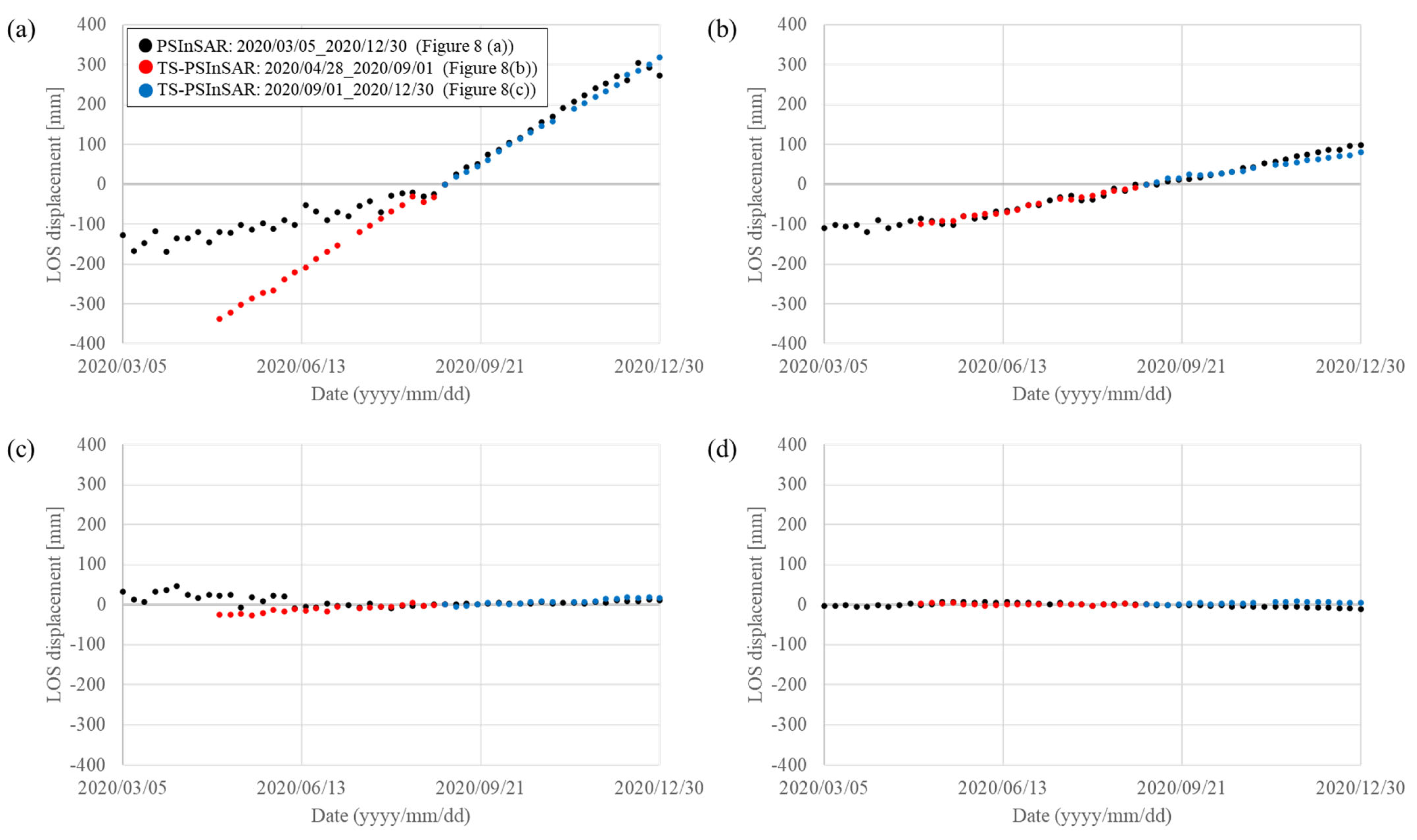
4.2. Time-Series Analysis Using Time Segmented PSInSAR (TS-PSInSAR)

As a result of applying the TS-PSInSAR techniques every 4 months, multiple PSs were observed in the study area for each time segment (Figure 12). In LOS velocity maps obtained as a result of TS-PSInSAR analysis, the maximum rate of rising from the center is slightly different with time, but the tendency to rise at a faster rate toward the center is the same. The vertical displacement of the CookE2 was obtained by connecting the relative displacements derived from each segment. Vertical displacements along the ICESat-2 track were obtained to compare with the TS-PSInSAR results (Figure 13). On 10 February 2020, data were acquired from both ICESat-2 and Sentinel-1. After selecting the point showing the lowest elevation in the ICESat-2 data on 10 February 2020, the ICESat-2 data of other periods and TS-PSInSAR results at the nearest location were extracted and plotted in time. ICESat-2 data were acquired from the right beam of each ground track out of six beams of track ID 695. Relative elevations obtained as a result of TS-PSInSAR have been converted to absolute elevations as of 10 February 2020.
Figure 13b shows the time series of the three points that match with ICESat-2 points. The slope of the linear regression of TS-PSInSAR was about (1) −0.03 m/year (R2 = 0.80), (2) 0.48 m/year (R2 = 0.99), and (3) 0.88 m/year (R2 = 0.99) for each point. The ICESat-2 observations are (1) 0.18 m/year (R2 = 0.83), (2) 0.80 m/year (R2 = 0.86), and (3) 1.17 m/year (R2 = 0.99), respectively.
Considering a conventional displacement error of half the wavelength (0.03 m), the uncertainty of the deformation rate for the linear regression during 28 months can be described as 0.01 m/year in the worst case. With 0.1 m measurement uncertainty for ICESat-2 for seven repeat cycles (636 days), the uncertainty of the deformation rate is 0.06 m/year. For the case of CryoSat-2 with 0.5 m of measurement uncertainty with the same duration, it would be 0.29 m/year. Therefore, the accuracy of TS-PSInSAR is far better than satellite altimeter data.

4.3. Recent Elevation Change by TS-PSInSAR

Finally, by referring to the satellite altimeter data, the time series change was investigated by converting the relative surface elevation displacement extracted through the InSAR technique into absolute elevation (Figure 14). Values were extracted from the center of the subglacial lake, where the most rapid change occurred for all points. Two ALOS DInSAR results in 2007 and 2010 were added. For the Sentinel-1 TS-PSInSAR results, we plotted the values by picking a point showing the maximum deformation rate. A vertical displacement of 2.54 m was confirmed at the center of the subglacial lake, and the average annual vertical uplift was about 1.10 ± 0.01 m/year (R2 = 0.99) for about 28 months from 2018 to 2021. The surface displacement of the center, measured with CryoSat-2, was approximately 1.18 ± 0.50 m/year between 12 February 2019 and 15 February 2020. Measurement by ICESat-2 gives an average rate of 1.17 ± 0.06 m/year. Observations with both altimeters are similar to TS-PSInSAR results, but the accuracy of TS-PSInSAR is superior to altimeter data.

5. Discussion

Summarizing the rationale of this study, the horizontal ice flow rate surrounding the CookE2 is rather slow as it is located near the ice divide. However, it was still problematic because it was of the same order as the vertical surface rise of CookE2, the target of this study. Individual DInSAR images had remaining linear phases due to local ice flow, which is difficult to estimate in each image. The removal of constant flow components through the DDInSAR is unlikely because the recent vertical rise of CookE2 has the same tendency. The main purpose of introducing the PSInSAR technique was to separate the surrounding ice flow from the vertical deformation of CookE2. As the deformation rate is too high in this study area, however, it is necessary to segment the duration of the dataset of PSInSAR into multiple segments and link them to extend the observation period. We call it TS-PSInSAR in this study, which require different duration or displacement limit for available data depending on the resolution of a SAR system and the deformation tendency.
This study suggests that the surface deformation during the segmented time of TS-PSInSAR should be less than 1/8 of the slant range resolution. Since the Sentinel-1 SAR system used in this study has a slant range resolution of about 2.4 m, the expected maximum displacement was 300 mm in 4 months for CookE2. In the case of TerraSAR-X with a 1.2 m slant range resolution, it would be 150 mm in 2 months. Similarly, when using the ERS-1/-2 data with 7.9 m slant range resolution, the segmented period can allow maximum deformation of 988 mm in 13 months.
The techniques used in this study are applicable to other subglacial lakes. Care must be taken to limit the maximum displacements to less than 1/8 of the slant range resolution of the SAR system when applied to other subglacial lakes. A priori information on the surface deformation of subglacial lakes is required. Although surface deformation of many active subglacial lakes is listed and reported, approximate displacement should be observed by altimeter data before applying TS-PSInSAR because anomalies could be changed at any time, not to mention the newly found subglacial lakes.
So far, elevation changes due to drainage of active subglacial lakes have been reported to take about two years or more [1]. The shortest previously reported subglacial lake drained in two months, and no lake had a shorter drainage period, probably due to the long revisit cycles of satellite altimeters. The existence of subglacial lakes, where discharge occurs more rapidly, cannot be completely ruled out. If the continuous and periodic observation data based on the satellite SAR system are utilized, it is expected that more detailed behavior of active subglacial lakes will be discovered. The entire displacement field can be observed by SAR so that even small subglacial lakes can be identified with high precision to lead to the discovery of many subglacial lakes in the near future.
CookE2 is recharging slowly after discharging relatively quickly. When subglacial water flows in, the water level will rise above the ridge point between the main lake and the hook-shaped zone of CookE2, confirmed through the radar-sounding data. Then, as the main lake and the hook-shaped zone are connected, it is expected that the surface change area of CookE2 will be expanded. If the elevation rises at a similar rate as the TS-PSInSAR results, it will reach the elevation just before the previous drainage in 40 years by 2060.

6. Conclusions

We analyzed the surface displacement of CookE2, one of the active subglacial lakes in East Antarctica, and detected the morphological features of the surface. Based on the ALOS PALSAR images, the DInSAR technique was applied to determine the surface displacement due to the rapid discharge of subglacial water. During the discharge, significant displacement occurred not only on the main lake but also on the hook-shaped zone. In 2007, a displacement of 8.00 ± 0.15 m in the main lake and 2.54 ± 0.15 m in the hook-shaped zone occurred in 46 days. The reason the two points have different rate is that the ridge point on the bedrock separates the two areas. The distribution of surface cracks due to such episodic subsidence can be detected by using the InSAR coherence image. Another ALOS PALSAR pair made it possible to confirm that a displacement of about 0.46 ± 0.15 m occurred over 46 days in 2010 when altimeter observation did not exist, making it clear that the subglacial lake was already in the process of recharging at that time. In addition, it was found that a displacement of 4.4 ± 0.8 cm occurred during 12 days in 2020 through the Sentinel-1 DInSAR image.
For the recent behavior of CookE2, more accurate vertical displacement could be found by applying the TS-PSInSAR. CookE2 has continued to rise linearly at a rate of 1.10 ± 0.01 m/year (R2 = 0.99) between September 2018 and December 2020. The horizontal deformation rate of 0.63 m/year from the flow velocity around the subglacial lake was successfully identified and removed by performing TS-PSInSAR. Since the temporal baseline of the Sentinel-1 data is shorter than satellite altimeters, it is possible to detect the subtle change in the upper surface of the subglacial lake. The proposed TS-PSInSAR measurement can provide much more accurate values of elevation change, but it cannot provide absolute elevation itself, which should be compensated by measurements from satellite altimeters.

Author Contributions

Conceptualization, J.M. and H.L. (Hoonyol Lee); methodology, J.M. and H.L. (Hoonyol Lee); software, J.M. and H.L. (Hoseung Lee); validation, J.M. and H.L. (Hoonyol Lee); formal analysis, J.M. and H.L. (Hoonyol Lee); investigation, J.M. and H.L. (Hoonyol Lee); resources, H.L. (Hoonyol Lee); data curation, J.M. and H.L. (Hoonyol Lee); writing—original draft preparation, J.M.; writing—review and editing, H.L. (Hoonyol Lee); visualization, J.M.; supervision, H.L. (Hoonyol Lee); project administration, H.L. (Hoonyol Lee); funding acquisition, H.L. (Hoonyol Lee) All authors have read and agreed to the published version of the manuscript.

Funding

This research was funded by [the National Research Foundation of Korea], grant number [NRF-2022R1F1A1071054, and No. 2019R1A6A1A03033167], and by [Ministry of the Interior and Safety as Human Resource Development Project in Disaster Management].

Data Availability Statement

The data presented in this study are available on request from the corresponding author.

Conflicts of Interest

The authors declare no conflict of interest.

References

  1. Livingstone, S.J.; Li, Y.; Rutishauser, A.; Sanderson, R.J.; Winter, K.; Mikucki, J.A.; Bjornsson, H.; Bowling, J.S.; Chu, W.N.; Dow, C.F.; et al. Subglacial lakes and their changing role in a warming climate. Nat. Rev. Earth Environ. 2022, 3, 106–124. [Google Scholar] [CrossRef]
  2. Pattyn, F. Antarctic subglacial conditions inferred from a hybrid ice sheet/ice stream model. Earth Planet. Sci. Lett. 2010, 295, 451–461. [Google Scholar] [CrossRef]
  3. Zwally, H.J.; Abdalati, W.; Herring, T.; Larson, K.; Saba, J.; Steffen, K. Surface melt-induced acceleration of Greenland ice-sheet flow. Science 2002, 297, 218–222. [Google Scholar] [CrossRef] [PubMed]
  4. Macgregor, K.R.; Riihimaki, C.A.; Anderson, R.S. Spatial and temporal evolution of rapid basal sliding on Bench Glacier, Alaska, USA. J. Glaciol. 2005, 51, 49–63. [Google Scholar] [CrossRef]
  5. Bell, R.E.; Studinger, M.; Shuman, C.A.; Fahnestock, M.A.; Joughin, I. Large subglacial lakes in East Antarctica at the onset of fast-flowing ice streams. Nature 2007, 445, 904–907. [Google Scholar] [CrossRef] [PubMed]
  6. Robin, Q.; Swithinbank, M.; Smith, B.M.E. Radio echo exploration of the Antarctic ice sheet. Int. Assoc. Sci. Hydrol. Publ. 1970, 86, 97–115. [Google Scholar]
  7. Siegert, M.J.; Dowdeswell, J.A.; Gorman, M.R.; McIntyre, N.F. An inventory of Antarctic sub-glacial lakes. Antarct. Sci. 1996, 8, 281–286. [Google Scholar] [CrossRef]
  8. Siegert, M.J. Antarctic subglacial lakes. Earth-Sci. Rev. 2000, 50, 29–50. [Google Scholar] [CrossRef]
  9. McMillan, M.; Corr, H.; Shepherd, A.; Ridout, A.; Laxon, S.; Cullen, R. Three-dimensional mapping by CryoSat-2 of subglacial lake volume changes. Geophys. Res. Lett. 2013, 40, 4321–4327. [Google Scholar] [CrossRef]
  10. Fricker, H.A.; Siegfried, M.R.; Carter, S.P.; Scambos, T.A. A decade of progress in observing and modelling Antarctic subglacial water systems. Philos. Trans. R. Soc. A Math. Phys. Eng. Sci. 2016, 374, 20140294. [Google Scholar] [CrossRef]
  11. Siegfried, M.R.; Fricker, H.A. Thirteen years of subglacial lake activity in Antarctica from multi-mission satellite altimetry. Ann. Glaciol. 2018, 59, 42–55. [Google Scholar] [CrossRef] [Green Version]
  12. Smith, B.E.; Fricker, H.A.; Joughin, I.R.; Tulaczyk, S. An inventory of active subglacial lakes in Antarctica detected by ICESat (2003–2008). J. Glaciol. 2009, 55, 573–595. [Google Scholar] [CrossRef]
  13. Fricker, H.A.; Scambos, T.; Bindschadler, R.; Padman, L. An active subglacial water system in West Antarctica mapped from space. Science 2007, 315, 1544–1548. [Google Scholar] [CrossRef]
  14. MacKie, E.J.; Schroeder, D.M.; Caers, J.; Siegfried, M.R.; Scheidt, C. Antarctic Topographic Realizations and Geostatistical Modeling Used to Map Subglacial Lakes. J. Geophys. Res. Earth Surf. 2020, 125, e2019JF005420. [Google Scholar] [CrossRef]
  15. Siegert, M.J.; Ridley, J.K. An analysis of the ice-sheet surface and subsurface topography above the Vostok Station subglacial lake, central East Antarctica. J. Geophys. Res. 1998, 103, 10195–10207. [Google Scholar] [CrossRef]
  16. Zwally, H.J.; Schutz, B.; Abdalati, W.; Abshire, J.; Bentley, C.; Brenner, A.; Bufton, J.; Dezio, J.; Hancock, D.; Harding, D.; et al. ICESat’s laser measurements of polar ice, atmosphere, ocean, and land. J. Geodyn. 2002, 34, 405–445. [Google Scholar] [CrossRef]
  17. Wang, F.; Bamber, J.L.; Cheng, X. Accuracy and performance of CryoSat-2 SARIn mode data over Antarctica. IEEE Geosci. Remote Sens. Lett. 2015, 12, 1516–1520. [Google Scholar] [CrossRef]
  18. Magruder, L.; Neuenschwander, A.; Klotz, B. Digital terrain model elevation corrections using space-based imagery and ICESat-2 laser altimetry. Remote Sens. Environ. 2021, 264, 112621. [Google Scholar] [CrossRef]
  19. Han, H.; Lee, H. Surface strain rates and crevassing of Campbell Glacier Tongue in East Antarctica analysed by tide-corrected DInSAR. Remote Sens. Lett. 2017, 8, 330–339. [Google Scholar] [CrossRef]
  20. Gray, L.; Joughin, I.; Tulaczyk, S.; Spikes, V.B.; Bindschadler, R.; Jezek, K. Evidence for subglacial water transport in the West Antarctic Ice Sheet through three-dimensional satellite radar interferometry. Geophys. Res. Lett. 2005, 32. [Google Scholar] [CrossRef]
  21. Capps, D.M.; Rabus, B.; Clague, J.J.; Shugar, D.H. Identification and characterization of alpine subglacial lakes using interferometric synthetic aperture radar (InSAR): Brady Glacier, Alaska, USA. J. Glaciol. 2010, 56, 861–870. [Google Scholar] [CrossRef] [Green Version]
  22. Palmer, S.; McMillan, M.; Morlighem, M. Subglacial lake drainage detected beneath the Greenland ice sheet. Nat. Commun. 2015, 6, 8408. [Google Scholar] [CrossRef]
  23. Neckel, N.; Franke, S.; Helm, V.; Drews, R.; Jansen, D. Evidence of Cascading Subglacial Water Flow at Jutulstraumen Glacier (Antarctica) Derived From Sentinel-1 and ICESat-2 Measurements. Geophys. Res. Lett. 2021, 48, e2021GL094472. [Google Scholar] [CrossRef]
  24. Lee, H.; Seo, H.; Han, H.; Ju, H.; Lee, J. Velocity Anomaly of Campbell Glacier, East Antarctica, Observed by Double-Differential Interferometric SAR and Ice Penetrating Radar. Remote Sens. 2021, 13, 2691. [Google Scholar] [CrossRef]
  25. Ferretti, A.; Prati, C.; Rocca, F. Nonlinear subsidence rate estimation using permanent scatterers in differential SAR interferometry. IEEE Trans. Geosci. Remote Sens. 2000, 38, 2202–2212. [Google Scholar] [CrossRef]
  26. Ferretti, A.; Prati, C.; Rocca, F. Permanent Scatterers in SAR interferometry. IEEE Geosci. Remote Sens. 2001, 39, 8–20. [Google Scholar] [CrossRef]
  27. Pandit, P.H.; Jawak, S.D.; Luis, A.J. Estimation of Velocity of the Polar Record Glacier, Antarctica Using Synthetic Aperture Radar (SAR). Proceedings 2018, 2, 332. [Google Scholar] [CrossRef]
  28. Flament, T.; Berthier, E.; Rémy, F. Cascading water underneath Wilkes Land, East Antarctic ice sheet, observed using altimetry and digital elevation models. Cryosphere 2014, 8, 673–687. [Google Scholar] [CrossRef]
  29. Li, Y.; Lu, Y.; Siegert, M.J. Radar sounding confirms a hydrologically active deep-water subglacial lake in east Antarctica. Front. Earth Sci. 2020, 8, 294. [Google Scholar] [CrossRef]
  30. Mouginot, J.; Rignot, E.; Scheuchl, B. MEaSUREs Phase-Based Antarctica Ice Velocity Map; Version 1 [Data Set]; NASA National Snow and Ice Data Center Distributed Active Archive Center: Boulder, CO, USA, 2019. [Google Scholar] [CrossRef]
  31. Mouginot, J.; Rignot, E.; Scheuchl, B. Continent-wide, interferometric SAR phase, mapping of Antarctic ice velocity. Geophys. Res. Lett. 2019, 46, 9710–9718. [Google Scholar] [CrossRef]
  32. Copernicus Space Component Data Access. Available online: https://spacedata.copernicus.eu/web/cscda/dataset-details?articleId=394198 (accessed on 4 August 2022).
  33. Wright, A.; Siegert, M. A fourth inventory of Antarctic subglacial lakes. Antarct. Sci. 2012, 24, 659–664. [Google Scholar] [CrossRef]
  34. Abdalati, W.; Zwally, H.J.; Bindschadler, R.; Csatho, B.; Farrell, S.L.; Fricker, H.A.; Harding, D.; Kwok, R.; Lefsky, M.; Markus, T.; et al. The ICESat-2 Laser Altimetry Mission. Proc. IEEE 2010, 98, 735–751. [Google Scholar] [CrossRef]
  35. Rosenqvist, A.; Shimada, M.; Ito, N.; Watanabe, M. ALOS PALSAR: A pathfinder mission for global-scale monitoring of the environment. IEEE Trans. Geosci. Remote Sens. 2007, 45, 3307–3316. [Google Scholar] [CrossRef]
  36. Rosenqvist, A.; Shimada, M.; Suzuki, S.; Ohgushi, F.; Tadono, T.; Watanabe, M.; Tsuzuku, K.; Watanabe, T.; Kamijo, S.; Aoki, E. Operational performance of the ALOS global systematic acquisition strategy and observation plans for ALOS-2 PALSAR-2. Remote Sens. Environ. 2014, 155, 3–12. [Google Scholar] [CrossRef]
  37. Rosenqvist, A.; Shimada, M.; Watanabe, M. ALOS PALSAR: Technical outline and mission concepts. In Proceedings of the 4th International Symposium on Retrieval of Bio- and Geophysical Parameters from SAR Data for Land Applications, Innsbruck, Austria, 16–19 November 2004. [Google Scholar]
  38. Potin, P.; Rosich, B.; Miranda, N.; Grimont, P.; Bargellini, P.; Monjoux, E.; Martin, J.; Desnos, Y.-L.; Roeder, J.; Shurmer, I. Sentinel-1 mission status. In Proceedings of the IEEE IGARSS, Milan, Italy, 26–31 July 2015; pp. 2820–2823. [Google Scholar]
  39. Torres, R.; Snoeij, P.; Geudtner, D.; Bibby, D.; Davidson, M.; Attema, E.; Potin, P.; Rommen, B.; Floury, N.; Brown, M.; et al. GMES Sentinel-1 mission. Remote Sens. Environ. 2012, 120, 9–24. [Google Scholar] [CrossRef]
  40. Sentinel Online. Available online: https://sentinels.copernicus.eu/web/sentinel/-/copernicus-sentinel-1b-anomaly-6th-update (accessed on 4 August 2022).
  41. Touzi, R.; Lopes, A.; Bruniquel, J.; Vachon, P. Coherence estimation for SAR imagery. IEEE Trans. Geosci. Remote Sens. 1999, 37, 135–149. [Google Scholar] [CrossRef]
  42. Goldstein, R.M.; Werner, C.L. Radar interferogram filtering for geophysical applications. Radio Sci. 1998, 25, 4035–4038. [Google Scholar] [CrossRef]
  43. Lee, H.; Seo, H. DInSAR signal of a subglacial lake in Wilkes Land, East Antarctica. In Proceedings of the AGU Fall Meeting, San Francisco, CA, USA, 9–13 December 2019. [Google Scholar]
  44. Seo, H.; Han, H.; Lee, H. Velocity Anomaly of David Glacier, East Antarctica, Observed by Double-Differential INSAR. In Proceedings of the IEEE IGARSS, Yokohama, Japan, 28 July–2 August 2019. [Google Scholar]
  45. Kim, H.; Han, H.; Lee, H. Uncharted Subglacial Lakes of David Glacier in East Antarctica Identified from Sentinel-1 DDInSAR and ICESat-2/CryoSat-2 Altimetry. In Proceedings of the AGU Fall Meeting, New Orleans, LA, USA & Online, 13–17 December 2021. [Google Scholar]
  46. Hooper, A.J.; Bekaert, D.; Hussain, E.; Spaans, K. StaMPS/MTI Manual; School of Earth and Environment: Leeds, UK, 2018. [Google Scholar]
  47. GIS-Blog. Available online: https://gitlab.com/Rexthor/gis-blog/-/blob/master/StaMPS/2-4_StaMPS-steps.md (accessed on 1 September 2022).
  48. Ice Bridge. Available online: https://www.nasa.gov/mission_pages/icebridge/instruments/mcords.html (accessed on 4 August 2022).
  49. Paden, J.; Li, J.; Leuschen, C.; Rodriguez-Morales, F.; Hale, R. IceBridge MCoRDS L3 Gridded Ice Thickness, Surface, and Bottom; Version 2 [Data Set]; NASA National Snow and Ice Data Center Distributed Active Archive Center: Boulder, CO, USA, 2013. [Google Scholar] [CrossRef]
  50. Paden, J.; Li, J.; Leuschen, C.; Rodriguez-Morales, F.; Hale, R. IceBridge MCoRDS L1B Geolocated Radar Echo Strength Profiles; Version 2 [Data Set]; NASA National Snow and Ice Data Center Distributed Active Archive Center: Boulder, CO, USA, 2014. [Google Scholar] [CrossRef]
Figure 1. The study area. (a) shows the location of CookE2 in the inventory of subglacial lakes beneath the Antarctica ice sheet [1]; (b) is an enlarged area of the green rectangle of (a), and shows the area of the SAR image used in this study (black, white, and yellow rectangle). In the legend of (b), the numbers in parentheses mean path and frame numbers, respectively. The cyan arrows indicate the direction and relative flow velocity of the ice flow; (c) is an enlarged area of the red-colored rectangle of (b), a shaded relief image of the CookE2 based on Copernicus 30 m DEM [32]. All subsequent figures are displayed in the same area as (c).
Remotesensing 14 04616 g001
Figure 2. Time series of elevation changes using altimeter data. ICESat and CryoSat-2 data were used in previous studies (reproduced after [9,12,28,29]) while ICESat-2 data were added in this study.
Remotesensing 14 04616 g002
Figure 3. Trend line comparison of Sentinel-1 time series vertical displacement using DInSAR and ICESat-2 altimeter data (modified from Lee and Seo [43]).
Remotesensing 14 04616 g003
Figure 4. Example images of DInSAR reprocessing: (a) the image before linear phase elimination; (b) estimated linear phase; and (c) the image after linear phase elimination.
Remotesensing 14 04616 g004
Figure 5. Example images of DDInSAR processing in the study area: (a) the DInSAR image from 24 September 2018; (b) the DInSAR image from 20 August 2020; and (c) the DDInSAR image from (a,b).
Remotesensing 14 04616 g005
Figure 6. Example images of orbital ramp removal: (a) time-series images of orbital ramps calculated in PSInSAR processing from September to December 2020; (b) the image before orbital ramps removal; and (c) the image after orbital ramps removal.
Remotesensing 14 04616 g006
Figure 7. Baseline plots of Sentinel-1 interferograms performed as a test. The red, blue, and grey lines are the baselines between the master image and the slave images.
Remotesensing 14 04616 g007
Figure 8. Comparison of PSInSAR result using 10-month data and TS-PSInSAR results using 4-month data: (a) mean LOS velocity map using 10-month data from March to December 2020; (b) mean LOS velocity map using 4-month data from May to August 2020; (c) mean LOS velocity map using 4-month data from September to December 2020. Each point indicated by A, B, C, and D is a point from which LOS displacement time series data were obtained in Figure 9, respectively.
Remotesensing 14 04616 g008
Figure 9. Time series of TS-PSInSAR according to the location of PS points in Figure 8: (a) LOS displacement in the center of the main lake; (b) LOS displacement in the edge of the main lake; (c) LOS displacement in the hook-shaped zone; and (d) the displacement at the point where the displacement assumed to be zero. The locations of the PS points are shown in Figure 8.
Remotesensing 14 04616 g009
Figure 10. Result images of DInSAR and coherence. (a,d) are DInSAR and coherence images using the ALOS PALSAR pair acquired on 15 November and 31 December, 2007; (b,e) are DInSAR and coherence images using the ALOS PALSAR pair acquired on 20 October and 5 December, 2010; (c,f) are DInSAR and coherence images using Sentinel-1 SAR pair acquired on 8 August 8 and 20 August, 2020. The white lines are cracks drawn based on (a,d).
Remotesensing 14 04616 g010
Figure 11. Radar sounding data from the MCoRDS5 airborne radar. (a) shows the path from which the radar sounding data was acquired. The black line represents the track in segment ID 04 and the white line represents frame number 010, which is part of it; (b) is the depth of ice bottom observed by MCoRDS5. Each A, B, and C represents the same point. The flight direction goes through A, and B, then through C.
Remotesensing 14 04616 g011
Figure 12. Mean LOS velocity maps using TS-PSInSAR. (a) is a baseline plot of interferograms used in TS-PSInSAR. The red dots are the master image of each segment while grey lines are linked to the slave images depicted as grey points. (bh) are mean velocity maps for each segment.
Remotesensing 14 04616 g012
Figure 13. The time series of TS-PSInSAR results. (a) is a map showing extraction points and observation track of ICESat-2. The track ID for ICESat-2 is 695. The background image is the mean LOS velocity map from September to December 2020, which is the same as Figure 12h; (b) represent the elevation according to time at points marked with the same color in (a).
Remotesensing 14 04616 g013
Figure 14. Comprehensive time-series result of elevation changes.
Remotesensing 14 04616 g014
Table 1. Results of previous studies [9,12,28,29].
StudyLake StatePeriod (yyyy/mm)dH (m)dH/dt (m/Year)dV (km3)Area (km2)
Smith et al. [9]Discharge2006/11~2008/0344~4833.5~36.5 *2.7146
McMillan et al. [12]Discharge2006/10~2008/107035 ± 146.36260
Recharge2008/10~2011/1017.2 ± 8.6 *5.6 ± 2.8-
Flament et al. [28]Discharge2006/11~2008/107036.0 *5.16 ± 1.52192~267
Recharge2008/10~2012/02133.9 *0.64 ± 0.32
Li et al. [29]Discharge2006/02~2008/1059.622.8 *2.7346
Recharge2011/01~2016/116.4 *1.10.42
* These values are estimated using data reported in papers.
Table 2. SAR data used in this study.
SatellitePathFrameAcquisition Date
(yyyy/mm/dd)
Acquisition ModeNumber of ScenesPerpendicular Baseline (m)Temporal Baseline (Days)
ALOS43556302007/11/15, 2007/12/31FBS2880.2146
2010/10/20, 2010/12/05FBS21030.3346
Sentinel-1549262018/09/12~2020/12/30IW112−148.89~108.616 or 12
Table 3. Changed StaMPS package parameters in this study (modified from Matthias Schlögl [47]).
ParameterDescriptionDefaultChanged
scla_derampThis parameter determines whether to estimate the phase ramp in each interferogram. If the phase ramp is estimated. It is subtracted before unwrapping.ny
unwrap_gold_n_winThis parameter determines the window size of Goldstein filtering performed before unwrapping [42].328
unwrap_grid_sizeAfter prefiltering before unwrapping, the grid spacing must be resampled. This parameter determines the grid spacing. Higher values reduce noise, but may cause undersampling.20010
unwrap_time_winThis parameter determines the smoothing window (in days) for smoothing the phase noise in time.73024
scn_time_winThis parameter determines temporal filtering (low-pass filtering) time window size for estimating the error.36550
Publisher’s Note: MDPI stays neutral with regard to jurisdictional claims in published maps and institutional affiliations.

