Can Satellite and Atmospheric Reanalysis Products Capture Compound Moist Heat Stress-Floods?

Abstract

Satellite-retrieved and model-based reanalysis precipitation products with high resolution have received increasing attention in recent decades. Their hydrological performance has been widely evaluated. However, whether they can be applied in characterizing the novel category of extreme events, such as compound moist heat-flood (CMHF) events, has not been fully investigated to date. The CMHF refers to the rapid transition from moist heat stress to devastating floods and has occurred increasingly frequently under the current warming climate. This study focuses on the applicability of the Integrated Multi-satellite Retrievals for Global Precipitation Measurement (IMERG) and the fifth generation of European Reanalysis (ERA5-Land) in simulating CMHF events over 120 catchments in China. Firstly, the precipitation accuracy of IMERG and ERA5-Land products is appraised for each catchment, using the gridded in situ meteorological dataset (CN05.1) as a baseline. Then, the ability of IMERG and ERA5-Land datasets in simulating the fraction, magnitude, and decade change of floods and CMHFs is comprehensively evaluated by forcing the XAJ and GR4J hydrological models. The results show that: (a) the IMERG and ERA5-Land perform similarly in terms of precipitation occurrences and intensity; (b) the IMERG yields discernably better performance than the ERA5-Land in streamflow simulation, with 71.7% and 50.8% of catchments showing the Kling–Gupta efficiency (KGE) higher than 0.5, respectively; (c) both datasets can roughly capture the frequency, magnitude, and their changes of floods and CMHFs in recent decades, with the IMERG exhibiting more satisfactory accuracy. Our results indicate that satellite remote sensing and atmospheric reanalysis precipitation can not only simulate individual hydrological extremes in most regions, but monitor compound events such as CMHF episodes, and especially, the IMERG satellite can yield better performance than the ERA5-Land reanalysis.

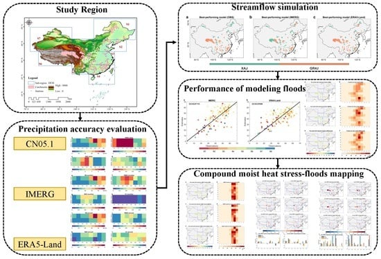
1. Introduction

As a critical component of the earth’s hydrological processes, precipitation is of key importance for the terrestrial ecosystem and human society [1]. Several measurements including in situ gauges and ground radar systems can provide highly accurate precipitation estimates. However, the sparse spatial distribution and expensive costs of gauges and radars limit their application, especially in rural areas [2]. Satellite remote sensing, advanced numerical weather models, and data assimilation systems provide new approaches in the trade-off between accurate precipitation estimation and large spatial coverage [3,4,5].

Since the launch of the Tropical Rainfall Measuring Mission (TRMM) in 1997, satellite precipitation estimates have been rapidly employed in hydrological fields [6,7,8]. As the first dataset of the four-dimensional distribution of rainfall over vast continents and oceans (50°S–50°N), the TRMM used to be the major user-friendly product that was widely applied in meteorological, hydrological, and agricultural sectors [9,10]. For example, Pombo and Oliveria [11] employed precipitation estimates from the TRMM to evaluate extreme precipitation in Angola and identified similar statistical characteristics to in situ ground observations. Following the highly successful TRMM, the Global Precipitation Measurement (GPM) mission was launched in 2014, which involves four critical components: the core observatory, the virtual constellation of satellites carrying precipitation-relevant sensors, the state-of-the-art precipitation processing system, and the ground validation [12]. Specifically, the Integrated Multi-satellite Retrievals for Global Precipitation Measurement (IMERG) employs a series of algorithms and processing sequences to merge all microwave, microwave-calibrated infrared satellite estimates, and gauge analyses, providing continuous precipitation records with high spatial (0.1°) and temporal (half hour) resolution at a global scale [13].

By using numerical weather models and data assimilation techniques, the model-based reanalysis product provides a new tool for global precipitation estimations [14,15]. The ERA5 released by the European Centre for Medium-Range Weather Forecasts (ECMWF) provides an enhanced global precipitation dataset (hereafter referred to ERA5-Land precipitation). Comparing to previous reanalysis datasets from ECMWF, e.g., the ERA-Interim, the ERA5-Land reanalysis uses a new 4D-Var assimilation algorithm and Integrated Forecasting System Cy41r2, which robustly improves its precision [16]. Further, this ERA5-Land precipitation provides a 0.1° spatial resolution at an hourly temporal scale spanning from 1950 to present. This high spatial and temporal resolution greatly facilitates its applications in water resources, land, and environmental management [17].

Numerous studies have examined the performance of satellite and reanalysis datasets under different temporal and spatial scales for a wide range of applications such as precipitation-phase partitioning and hydrological modeling [18,19,20]. For example, Gao et al. [4] evaluated the accuracy of recently released satellite and reanalysis precipitation over southern China at daily and hourly scales and found that their performances were varied when assessed at different temporal scales. Xu et al. [16] analyzed the performances of several satellite and reanalysis precipitation products over mainland China and concluded that satellite precipitation outperforms reanalysis in tropical monsoon climates, while the latter shows better performance over temperate monsoon climate and high-latitude regions. Tang et al. [2] focused on the quality of snowfall estimates in satellite and reanalysis datasets from 2000 to 2018 and found the IMERG product performs well, and its performance has improved over time due to the increasing passive microwave samples. For hydrological application, Jiang et al. [18] claimed that the IMERG precipitation can be applied in streamflow monitoring, especially in humid catchments. Almagro et al. [5] found the GPM products perform well in simulating river discharge over tropical catchments. However, most studies only employed statistical indices to appraise the performance of satellite and reanalysis products in capturing precipitation events, or to evaluate the applicability of these products in simulating streamflow conditions. Their ability in characterizing floods, especially in quantifying the novel category of extreme events, such as the compound moist heat-flood (CMHF) events, has been poorly understood.

Flooding is one of the most prevalent natural hazards, causing multifaceted challenges to the ecosystem, agriculture, economy, and society [21,22,23,24]. For example, the flood that occurred in the Henan province of China in 2021 caused USD 348 million of economic losses and killed 6.4 million chickens. As earth’s climate is warming, in addition to flood, the flood-related compound disaster, has also become increasingly apparent (e.g., the rapid transition from moist heat stress to floods) [25,26]. Compared to an individual flood extreme, such compound events are far more destructive to human health and societies [27,28,29]. For example, the consecutive occurrence of heat stress and floods in 2019, Queensland, caused half a million livestock deaths and huge amounts of economic losses [26]. Therefore, this study aims to comprehensively investigate the applicability of satellite remote sensing (IMERG) and reanalysis (ERA5-Land) datasets in monitoring flood seasons and magnitudes, particularly in quantifying characteristics of CMHF episodes for 120 catchments varying in climate zones and streamflow generation regimes in China from 2001 to 2020. We first evaluate the performances of the IMERG and ERA5-Land precipitation, using a gridded observation product as a baseline. Then, their performances in hydrological simulations are also assessed by using two lumped hydrological models. Finally, we investigate the reliability of the IMERG and ERA5-Land in capturing flood extremes, with special attention paid to simulating CMHF fraction, magnitude, and changes.

2. Materials and Methods

2.1. Dataset

2.1.1. Meteorological Dataset

The IMERG precipitation was obtained by combining information from the TRMM (2000–2015) and GPM (2014–present) satellite constellation with an advanced algorithm [12]. It provides the early, late, and final runs with half-hourly temporal and 0.25° spatial resolution. Since the final run utilizes multiple sources of information, including multi-satellite data and a GPCC gauge, and is recommended by NASA for research, we employed the final run precipitation in IMERG in this study.

The ERA5-Land developed by the ECMWF is a reanalysis dataset using a state-of-the-art scheme (incorporating land surface hydrology, H-TESSEL) for surface exchanges over land [17]. It provides various land variables with super high spatial (0.1°) and temporal (hourly) resolution from 1950 to present. This global reanalysis dataset combines observations with model data using physical laws and is forced by atmospheric constraints. We used its precipitation spanning 2001–2020 to serve as a comparison to IMERG in this study. The hourly IMERG and ERA5-Land precipitation were integrated into the daily scale for analysis.

The gridded observational meteorological data were CN05.1 constructed by the China Meteorological Administration [30], which incorporates information from 2416 gauges in China and has been widely used as an observational reference in recent studies [31,32,33]. It provides daily temporal and 0.25° spatial resolution spanning 1961–2020. Seven variables are included in this dataset, i.e., precipitation, relative humidity, windspeed, sunshine hours, and daily maximum, minimum, and average temperature. Relative humidity (RH) and daily temperature (T) were used in this study to estimate moist heat stress. Precipitation and daily maximum, minimum, and average temperature were used to calibrate hydrological models.

2.1.2. Observed Streamflow Data

To evaluate satellite and reanalysis precipitation in hydrological simulation, 120 catchments with different hydro-meteorological conditions were selected (Figure 1). These catchments have no overlapping area, and each catchment matches with only one station. The boundaries of these catchments as well as their daily streamflow records between 2001 and 2010 were collected from the Ministry of Water Resources of China. All catchments contain at least 5-year continuous daily streamflow records and 88.33% of catchments have consistent daily records longer than 7 years (for more details, see Figure S1). There were only three catchments (which have 8-, 7-year records) involving missing data, with missing ratios being 2.6%, 9.2%, 0.3%, respectively. Eight sub-regions in China that synthetically consider the monsoon climate characteristics, agricultural geographical distributions, and topography were used to facilitate assessment [34,35] following previous studies [36,37,38,39]. It should be mentioned that the number of streamflow stations allocated in Northeast China, North China, Jiang-Huai Region, South China, and Southwest China (S1–S5) dominate the population of gauges. Geographically wise, our study cannot well represent conditions in the Tibetan Plateau and Northwest China (S6–S8) due to data limitation. The spatial distribution of the catchments located in the eight sub-regions is plotted in Figure 1.

2.2. Methods

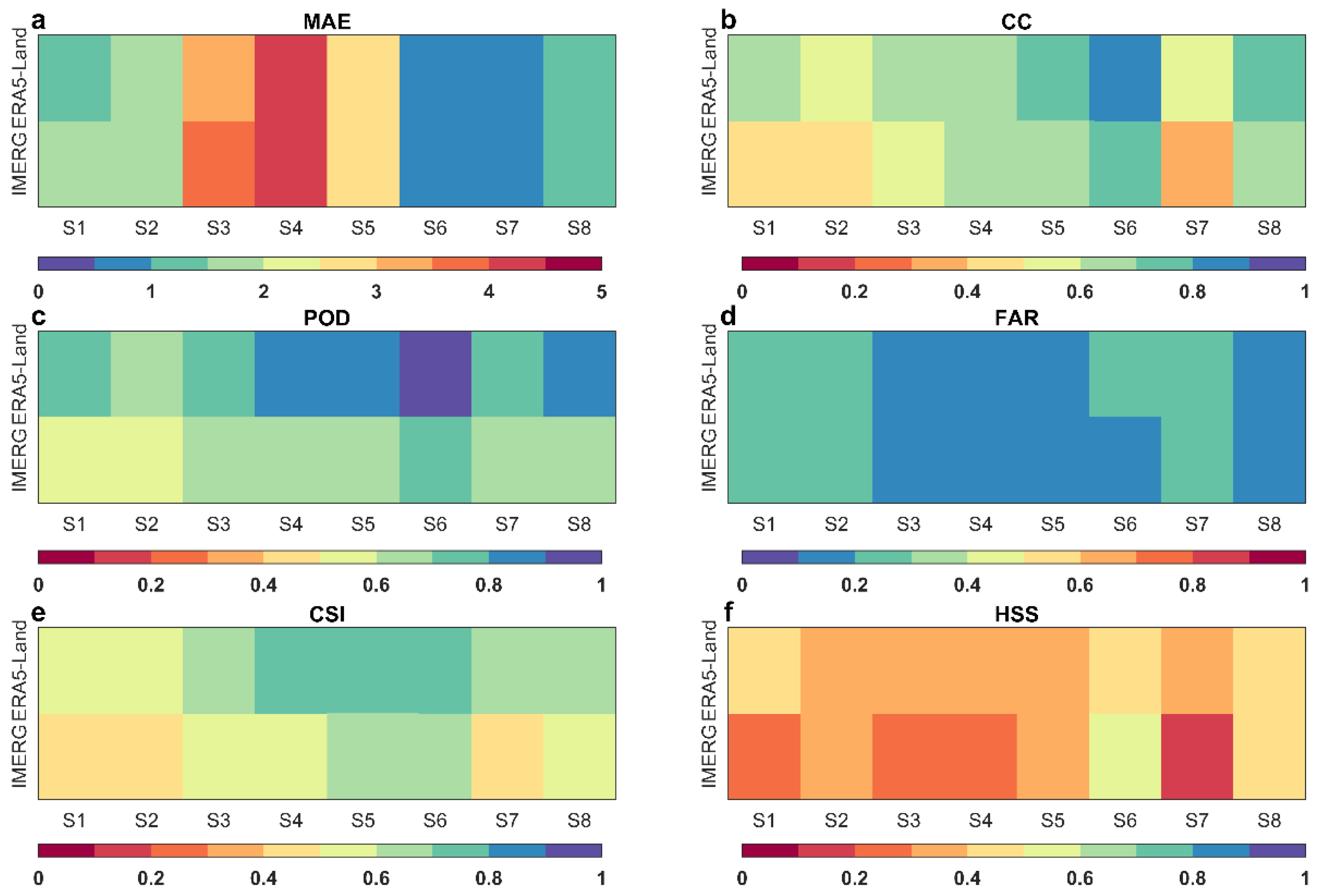
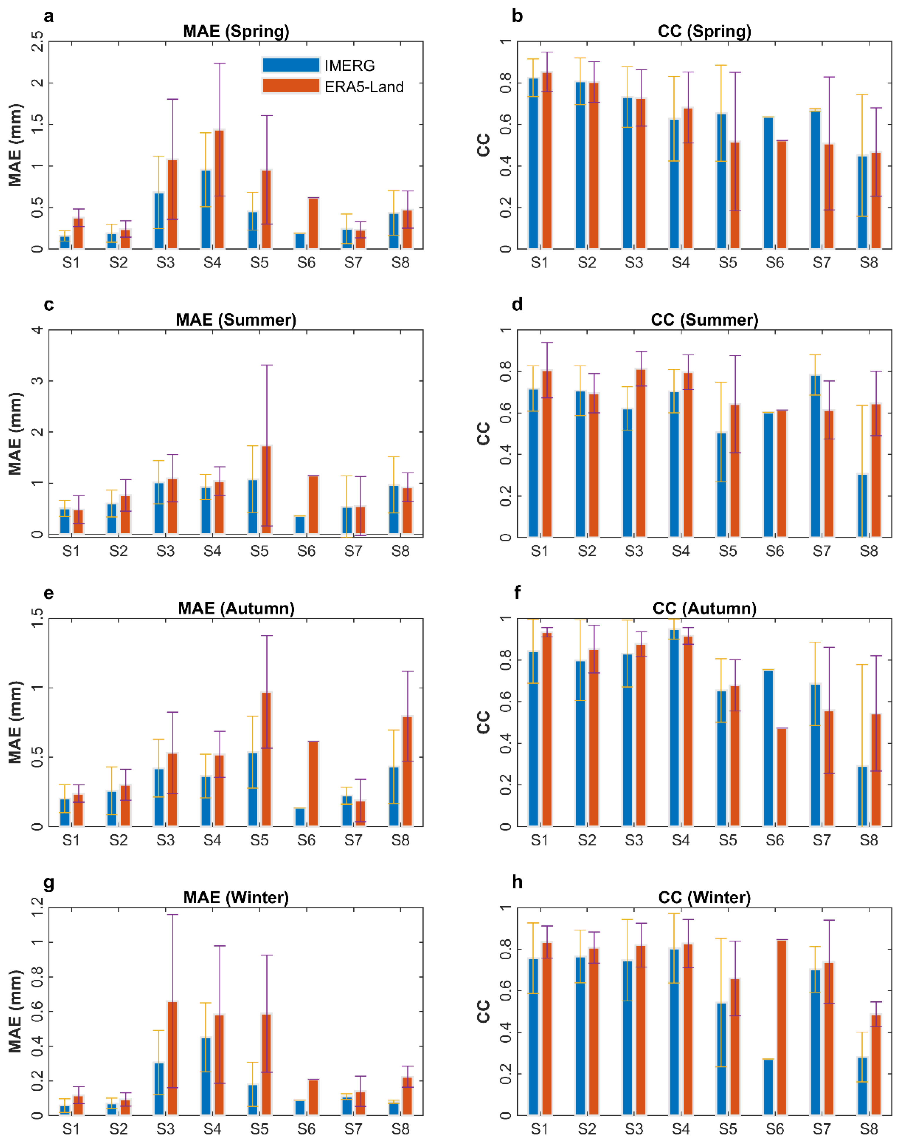
2.2.1. Precipitation Indices for Evaluating Precipitation Estimation Accuracy

Six indices (expressed in

Table 1. Definitions of the statistical indices in evaluating the accuracy of precipitation datasets. The final column indicates the perfect score for each index.

ID	Index	Expression	Description	Perfect Score
1	MAE	$\frac{{\displaystyle {\sum }_{i=1}^N\left|S_i-O_i\right|}}{N}$	mean absolute error	0
2	CC	$\frac{{\displaystyle {\sum }_{i=1}^N(S_i-\overline{S})(O_i-\overline{O})}}{\sqrt{{\displaystyle {\sum }_{i=1}^N{(S_i-\overline{S})}^2}}\times \sqrt{{\displaystyle {\sum }_{i=1}^N{(O_i-\overline{O})}^2}}}$	correlation coefficient	1
3	POD	$\frac{a}{a+c}$	probability of detection	1
4	FAR	$\frac{b}{a+b}$	false alarm ratio	0
5	CSI	$\frac{a}{a+b+c}$	critical success index	1
6	HSS	$\frac{2(a\times d-b\times c)}{[(a+c)\times (c+d)+(a+b)\times (b+d)]}$	Heidke skill score	1

Note: S_i and O_i denote simulated and observed daily precipitation in i (i = 1,2,…N) day; $\overline{S}$ and $\overline{O}$ denote the mean value of simulated and observed precipitation among N days.

) were used to estimate the accuracy of IMERG and ERA5-Land precipitation. Two indices, MAE and CC, focus on the precision of precipitation intensity while the other four indices, POD, FAR, CSI, and HSS, target the detection of the occurrence of precipitation. Specifically, the last four indices, POD, FAR, CSI, and HSS, are estimated by four parameters: a, the number of wet days (i.e., precipitation occurs) correctly detected; b, the number of dry days (i.e., no precipitation) erroneously identified as wet days; c, the number of missing wet days; d, the number of dry days correctly detected. The POD, CSI, and FAR are highly affected by wet days. In detail, the POD and CSI present the ability of simulations in capturing precipitation occurrence while the FAR measures the false ratio of erroneously simulated precipitation on dry days. The HSS, on the other hand, accounts for information from both wet and dry days when detecting the accuracy of precipitation occurrence.

2.2.2. Hydrological Simulations

In terms of hydrological simulation, firstly, we calculated the catchment average meteorological data including precipitation (i.e., the IMERG, ERA5-Land, and CN05.1), and maximum and minimum temperature (i.e., CN05.1) using the Thiessen polygon method for the 120 catchments in mainland China. This utilization of the Thiessen polygon method can better allocate weights for grids intersected by catchment boundaries than the arithmetic average method, following previous studies (e.g., Yin et al., 2021 [40]), and can guarantee correct weights for grids inside boundaries. Then, we used two precipitation products (i.e., the IMERG and ERA5-Land) and observations (i.e., CN05.1) to calibrate hydrological models, respectively. We chose two lumped hydrological models, the Xinanjiang (XAJ) [41] and GR4J [42], to perform streamflow simulations over these catchments. The XAJ and GR4J models vary in model structures and parameters and can consider different climate conditions and runoff generation regimes, having been proved to perform well in China by previous studies [40,43,44]. Specifically, the XAJ rainfall-runoff model comprises 15 free parameters and separates the watershed area into pervious and impervious area. For the pervious area, the effective rainfall is separated into three sources: surface runoff, interflow, and groundwater, while for the impervious area, the effective rainfall totally transfers to surface runoff. The GR4J model is a simple rainfall-runoff model consisting of 4 free parameters. It only involves two non-linear reservoirs and two linear unit hydrographs when simulating runoff generation and routing. The potential evaporation module, the Oudin equation [45], is employed for both the XAJ and GR4J models. Further, to simulate snowmelt-runoff, the two-parameter CemaNeige snow accumulation and snowmelt module [46] is incorporated into the XAJ and GR4J models. This CemaNeige module involves 2 free parameters. Firstly, it separates precipitation into rainfall and snowfall, and then it calculates the snowmelt using a degree-day method.

We employed the Shuffled Complex Evolution (SCE-UA) optimization algorithm [47] to determine the free parameters of hydrological models. The SCEUA is a powerful global optimization procedure. It considers both deterministic and random search and is capable of efficiently and effectively identifying the optimal values for model parameters. Specifically, a cross-validation method was selected for model evaluation, in which half of the daily streamflow records were used as the calibration and the other half of records were for validation [41,48]. Further, the objective function in model calibration is to maximize the Kling–Gupta efficiency (KGE) [49] of daily streamflow for each catchment, respectively:

$$KGE=1-\sqrt{{(\alpha -1)}^2+{(\beta -1)}^2+{(\gamma -1)}^2}$$

(1)

where α denotes the correlation coefficient, β refers to the ratio of standard deviations, and γ means the ratio of mean values between daily streamflow records and simulations, respectively. For each catchment, the model (XAJ or GR4J) with the highest KGE value in both calibration and validation periods was determined as the best performing model. Then, the best performing models were forced by the observation (CN05.1), IMERG, and ERA5-Land products, respectively, to obtain daily streamflow during the 2001–2020 period. Since we only collected a limited length of in situ streamflow observations over these catchments (ranging between 2001 and 2010, see Figure S1), which cannot cover the whole 2001–2020 time period, the streamflow simulated by observed climate data (CN05.1) was used as the new observation baseline to perform further hydrological analysis following previous studies [48,50,51].

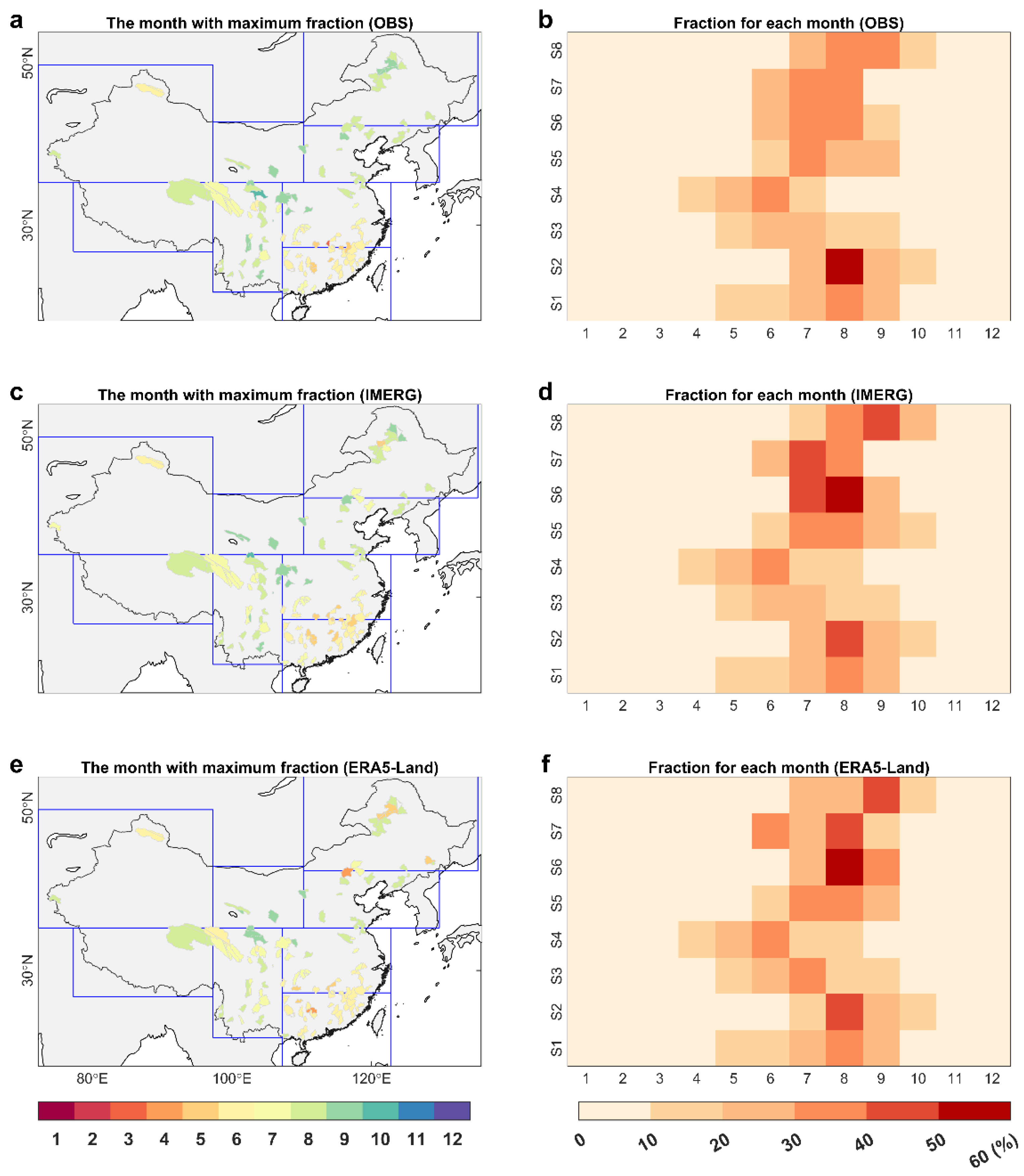
2.2.3. Identifying Compound Moist Heat-Flood Events

We employed a peak-over-threshold (POT) approach to extract flood episodes. A flood occurs when daily streamflow is higher than a threshold (95th percentile of the whole time series in this study, Q^95th) during the 2001–2020 period and terminates when streamflow becomes lower than the threshold. The cumulative streamflow above the threshold denotes a flood magnitude (M):

$$M={\displaystyle \sum _{i=1}^t{Q}_i-Q^{95\mathrm{th}}}$$

(2)

where Q_i denotes the streamflow in i (i = 1,2,…t) day during a flood episode, t is the length of an episode. We investigated the flooding fraction (monthly average flood counts versus total counts) and magnitude (monthly and annual average flood magnitude) to quantify floods simulated by observations, the IMERG, and ERA5-Land. We also calculated the changes in flooding fraction (Δfraction^Flood) and magnitude (Δmagnitude^Flood) in each catchment between 2001–2010 and 2011–2020 (the latest period minus the previous period) to fully evaluate the ability of satellite and reanalysis products in simulating floods.

The wet-bulb temperature was used to estimate moist heat stress (T_wb) [52]:

$$\begin{array}{l}{T}_{wb}=T\times \arctan (0.151977\times {(RH+8.313659)}^{1/2})+\arctan (T+RH)\\ -arctan(RH-1.676331)+0.00391838\times {(RH)}^{3/2}\times \arctan (0.023101\times RH)-4.686035\end{array}$$

(3)

where T denotes near-surface temperature and RH denotes relative humidity; both of them were derived from the CN05.1 dataset. Then, a moist heat extreme was defined based on the T_wb time series and the POT approach, similar to the procedure in defining floods, and the 95th percentile of the whole time series, $T_{wb}^{95\mathrm{th}}$, was determined as the threshold. Finally, a compound moist heat-flood episode was defined as when a flood is preceded by a moist heat extreme within seven days:

$$\begin{array}{l}CMHF=({\displaystyle \sum _{i=a}^n{Q}_i-Q^{95\mathrm{th}}},{\displaystyle \sum _{j=b}^m{T}_{wb,j}-T_{wb}^{95\mathrm{th}}})\\ \begin{array}{c}a-m>0,a-m<=7 \mathit{or} a-b>0,a-m<=7\end{array}\end{array}$$

(4)

where T_wb,j (Q_i) denotes a moist heat stress (flood) starting from date j (i) and ending at date m (n), and other abbreviations are as described above. We calculated the monthly and total CMHF fraction, the monthly and total average counts of CMHF events versus the monthly and total average counts of floods, and the monthly and total CMHF magnitude (since the magnitude in moist heat stress is totally estimated by CN05.1, here we only focused on the magnitude of the flooding side in a CMHF event) to characterize CMHF events. Further, we also used the changes of the CMHF fraction (Δfraction^CMHF) and magnitude (Δmagnitude^CMHF) to evaluate the accuracy of IMERG and ERA5-Land in application to CMHF modeling.

3. Results

3.1. Performance Assessments of IMERG and ERA5-Land Precipitation

To assess the performance of IMERG and ERA5-Land products, we used six indices to detect their precipitation intensity (MAE and CC) and occurrence (POD, FAR, CSI, and HSS). We estimated these indices for each catchment in the eight regions of mainland China (Figures S2 and S3) and present the regionally averaged values in Figure 2. In terms of the MAE metric, the IMERG performs similarly to the ERA5-Land, with values ranging from 0.7 to 5.0 mm and from 0.8 to 4.9 mm, respectively. The MAE values are larger in south China (S3–S5), mainly attributed to local heavy precipitation conditions [35]. In contrast, the ERA5-Land shows better performance with regard to the CC metric. Specifically, the CC metric ranges from 0.54 to 0.81 in daily ERA5-Land precipitation, while it only ranges from 0.34 to 0.73 in the IMERG. The IMERG product cannot effectively catch precipitation characteristics, especially in north China (S1, S2, and S7). From the precipitation occurrence perspective, different metrics demonstrate varying results. For instance, the IMERG exhibits lower FAR and higher HSS values than the ERA5-Land, indicating slightly better performance. However, the POD and CSI metrics show the opposite results.

To further probe into satellite and reanalysis precipitation performance, we employed MAE and CC metrics to evaluate seasonal precipitation intensity (Figure 3). Generally, both products exhibit acceptable accuracy in all seasons over catchments in China. The MAE metric varies from 0.04 to 1.86 mm (from 0.06 to 3.2 mm) for IMERG (ERA5-Land) daily seasonal precipitation. The Jiang-Huai Region, and South and Southwest China (S3–S5), generally yield larger MAE than the other sub-regions. This is mainly because the index MAE is highly sensitive to local precipitation amount and is spatially heterogeneous. The IMERG and ERA5-Land thus produce relatively large MAE in the S3–S5 in which they show a wet climate. With regard to the CC metric, values in IMERG approximately vary between 0.27 and 0.95, and vary between 0.47 and 0.93 in ERA5-Land. Spatially, both the IMERG and ERA5-Land exhibit almost homogeneous performance among eight regions. We further estimated additional metrics including daily, monthly, and annual indices to fully measure the accuracy of IMERG and ERA5-Land precipitation products (Figure S4). We found different indices and different timescales typically yield varied results: the IMERG presents higher accuracy than the ERA5-Land in terms of monthly and annual indices, while the ERA5-Land shows more accurate precision in simulating precipitation occurrence. Overall, the results above demonstrate the reliability of IMERG and ERA5-Land precipitation products in China despite a few catchments showing inferior performance, motivating us to further investigate their applicability in the hydrological field.

3.2. Calibration and Validation of Hydrological Models

Considering different climatic and underlying surface conditions for different catchments, we employed two hydrological models, the XAJ and GR4J models, to investigate the applicability of the IMERG and ERA5-Land in streamflow simulations. Specifically, the observations (CN05.1), IMERG, and ERA5-Land were all used to calibrate these two hydrological models and the best performing model (with the highest KGE value) was selected for each dataset and catchment to perform further flood simulations. The best performing hydrological models were different among three precipitation datasets. The GR4J model performs better over the majority of catchments when forced by CN05.1 (64.2% of catchments) and ERA5-Land (71.7% of catchments) datasets, while the XAJ model yields slightly better performance when forced by IMERG precipitation, as indicated by higher KGE values in 56.7% of catchments (Figure S5).

As expected, the hydrological models achieve the best performance when forced by the observation dataset (CN05.1), with around 85% of catchments exhibiting a KGE higher than 0.5 and around 71.7% of catchments showing a KGE higher than 0.7 during both calibration and validation periods (Figure 4a,b). This indicates the robustness of the observation dataset and best performing models. In contrast, though the KGE is lower when driven by IMERG, they are still satisfactory to some extent. There are around 71.7% of catchments yielding a KGE higher than 0.5 and 50.8% of catchments demonstrating a KGE higher than 0.7 during calibration and validation periods, implying the potential of IMERG serving as an alternative in hydrological modeling over catchments in China (Figure 4c,d). On the other hand, although the ERA5-Land exhibits similar precision to the IMERG according to the above six precipitation indicators, it performs worse than the IMERG in simulating streamflow. We observe only 50.8% of catchments yielding a KGE higher than 0.5 and 33.3% of catchments having a KGE higher than 0.7 (Figure 4e,f). This demonstrates the non-linear transferability from climates to hydrological variables and indicates that good climate performance may not sufficiently facilitate hydrological modeling. To probe into water balance issues in modeling performance, we further estimated relative bias of hydrological simulations by the OBS, IMERG, and ERA5-Land against streamflow records across the whole calibration and validation periods for these catchments (Figure S4). Generally, despite some underestimation (overestimation) by the OBS and IMERG (the ERA5-Land), the relative biases range between −5.4% and 6.9%, indicating the reliability of streamflow simulations.

3.3. Performance of Modeling Extreme Streamflow

Before touching on the applicability of IMERG and ERA5-Land in CMHF episodes, we firstly investigated the ability of simulated streamflow in capturing flooding characteristics during the 2001–2020 period. We extracted flood episodes for each catchment from CN05.1, IMERG, and ERA5-Land, respectively, and used results from CN05.1 as a baseline. The total flood frequency approximately ranges from 10 to 70 times in these catchments during the 2001–2020 period. The IMERG and ERA5-Land can basically reproduce the flood frequency, with the correlation coefficients of 0.67 and of 0.58, respectively (Figure S7). We further investigated the flood fraction for each month (i.e., the floods that occurred in each month against total counts) and identified the month with the maximum fraction (Figure 5 and Table S1). As expected, floods mainly occur in the warm season (e.g., May to September) and the month with the maximum flooding fraction is typically earlier in southeast China (e.g., early-monsoon, May–June) than the northern catchments (e.g., monsoon, July–September) (Figure 5a). Generally, the IMERG can better reproduce this spatial pattern than the ERA5-Land (Figure 5c,e). From a spatially averaged perspective, floods occurred most frequently in July and August, as indicated by 23.5% and 26.5% of flooding fractions (Figure 5b). The fraction results for the IMERG are highly similar to those from observations, though they to some degree overestimate flooding fractions in July and August for catchments in S7 and S8 and underestimate them for catchments in S2 (Figure 5d). Again, the differences of flooding fraction for the ERA5-Land against the observations are larger than for the IMERG. For instance, the spatially averaged fractions in July and August are 20.8% and 28.7% for the ERA5-Land, while they are 25.2% and 26.3% for the IMERG during the 2001–2020 period.

We further investigated fraction change (Δfraction^Flood) in the warm season and changes in recent decades. The results for July and the decade in these catchments are shown in Figure 6. The flood fraction in southeast China (S3–S4) shows a decrease in July, while it shows an apparent increase in west and northwest China (S6–S8) (Figure 6a). The IMERG can roughly reproduce the spatial pattern of fraction changes in July (Figure 6c). For ERA5-Land, however, apparent discrepancies against results from observations are observed in northeast (S1–S3) and west (S6) China, demonstrating the limitation of the ERA5-Land product in flood modeling (Figure 6e,g). We also estimated fraction change in May, June, August, and September (Figures S8 and S9). Generally, both the IMERG and ERA5-Land demonstrate similar spatial patterns of monthly fraction change to those from observations, and results from the IMERG resemble more closely those observations than those from the ERA5-Land. In terms of decade change, there is a drastic nationwide increase in the flood fraction, and the spatially averaged value is around 130% (Figure 6b). However, both IMERG and ERA5-Land show only slight increases or even decreases in decadal fraction change, with the national average value for all catchments being around 16.9% and 0.9%, respectively (Figure 6d,f,h)

Large floods typically occur during the monsoon season (e.g., July, August, and September), and around 63.3% of catchments exhibit maximum flood magnitude during these months (Figure 7a). Spatially, more severe floods are observed in east China, especially in S3–S4 (Figure 7b). For IMERG and ERA5-Land, almost similar spatial patterns to observations in the month with maximum magnitude are observed (Figure 7c,e). Furthermore, monthly flood magnitudes driven by IMERG and ERA5-Land are also analogical to observations (Table S2). The spatially averaged flood magnitude is 17.2 mm in observations (averaged by each month, Figure 7b), and is approximately 18.6 and 14.8 mm in IMERG and ERA5-Land (Figure 7d,f), again demonstrating the more satisfactory performance of IMERG than of ERA5-Land in modeling flood magnitudes.

There is a nationwide increase in flood magnitudes (△magnitude) in July and the spatial average value is approximately 102.2% (Figure 8a). The increase in flood magnitude in July is much greater in northeastern (S1–S2) and southwestern (S5–S6) catchments than in other regions. The IMERG underestimates the sharp increase in flood magnitudes in July, with the spatial average value of around 60.1% (Figure 8c). For ERA5-Land, the nationwide increasing phenomenon in flood magnitudes is also not evident. Specifically, the ERA5-land exhibits decreasing changes in S4 where most catchments should present increasing changes (Figure 8e). In other warm season months (e.g., May, June, August, and September), the IMERG and ERA5-land can reluctantly reproduce the spatial patterns of △magnitude, though with discernable differences in the changing magnitudes (Figures S10 and S11). On the other hand, changes in flood magnitudes from the annual perspective are observed to be less severe than those in July, where the spatial average value is only 52.3% (Figure 8b). The IMERG basically exhibits a similar spatial pattern to the observations, despite some overestimation in the increasing magnitudes. By contrast, a remarkable underestimation in annual magnitude changes and even opposite changing directions are observed in ERA5-Land (Figure 8f). Overall, the IMERG roughly shows analogical flood characteristics to the observations, while the ERA5-Land cannot reliably simulate floods.

3.4. CMHF Mapping and Performance Assessment

We first investigated the frequency of CMHF during the 2001–2020 period over catchments in China from observations, IMERG, and ERA5-Land, respectively (Figure 9). The frequency of CMHF from IMERG (or ERA5-Land) shows significant positive correlations with that from the observations, indicating the good performance of IMERG (or ERA5-Land) in simulating CMHF frequency.

There is a similar story in terms of the CMHF fraction (Figure 10 and Table S3). For the CMHF fraction, 91.7% of catchments show the maximum CMHF fraction in the hot months (e.g., July–August) (Figure 10a,b). This is mainly due to the fact that moist heat stress can only occur in warm seasons in China, resulting in a super high concentration of CMHF in July and August. Both the IMERG and ERA5-Land effectively capture the pattern of the CMHF fraction, as indicated by 95.0% and 89.2% of catchments exhibiting maximum CMHF fraction in the hot months, respectively (Figure 10c–f). Furthermore, we observe more catchments exhibiting increases in both monthly and annual CMHF fraction (Figure 11a,b). In other words, more CMHF events occurred in the recent 2001–2010 decade than in the previous 2011–2020 period, indicating potentially deteriorating CMHF hazards. Again, these changes in the CMHF fraction are robustly captured by the IMERG and ERA5-Land (Figure 11c–h).

To better understand the applicability of IMERG and ERA5-Land in capturing CMHF characteristics, the flood magnitude in each CMHF episode was extracted. The monthly magnitudes of floods preceded by moist heat stress and their changes are presented in Figure 12 and Figure 13 and Table S4. As expected, the majority of catchments show maximum CMHF magnitude in the warm seasons, July–September, accounting for 89.2%, 92.5%, and 93.3% of catchments in observations, IMERG, and ERA5-Land products, respectively (Figure 12a,c,e). Nevertheless, it should be noted that a larger CMHF magnitude typically emerges in the post-monsoon season (September–October). Specifically, the spatially averaged CMHF magnitudes are around 43.2 and 61.4 mm in September and October, respectively (Figure 12b), much larger than those in July (17.8 mm) and August (15.9 mm). The IMERG basically captures this pattern of larger magnitudes in post-monsoon seasons than in monsoon seasons (Figure 12d), while the ERA5-Land fails to reproduce severe CMHF magnitudes that emerged in October (Figure 12f). For changes in CMHF magnitudes, increases can be observed in July and annual scales over most catchments, with a spatially averaged value of 83.1% and 169.1%, respectively (Figure 13). Both the IMERG and ERA5-Land can reproduce these spatial patterns, despite some disparities in the changing magnitudes. Specifically, the ERA5-Land drastically underestimates the increases in annual CMHF magnitudes, with a spatially averaged value of only 21.2%. The IMERG again simulates a more analogical change in annual CMHF magnitudes, and the spatial average increase is approximately 98.4%. Overall, the IMERG and ERA5-Land can generally simulate the spatial patterns of CMHF seasons, magnitudes, and their changes, with the IMERG exhibiting slightly better performance than the ERA5-Land. However, some differences still exist in the timing and magnitudes of CMHF episodes simulated by IMERG and ERA5-Land to that by observations, and caution should be paid when directly using these products to investigate compound hazards.

4. Discussion

Recent studies have examined characteristics of similar compound extremes [29,53,54]. For example, Ning et al. [31] investigated the characteristics of compound extreme heat-precipitation events across China during 1961–2016 and found around one-quarter of summer precipitation extremes over China are preceded by an extreme heat event. Based on previous studies, we took a step further to fully investigate the intra-annual distribution of the proportions and magnitudes of floods that are preceded by moist heat stress. Interestingly, though we observed large CMHF fractions that typically emerged in July and August, CMHF episodes with severe magnitudes prominently occurred in post-monsoon seasons, i.e., September to October, in which the average magnitudes were more than double the magnitudes in July and August (Figure 12b).

It is noteworthy to mention that we used the wet-bulb temperature rather than the dry-bulb temperature to consider the deadly heat stress in this study, which is different from most previous compound heat-flood studies [31,53]. This wet-bulb temperature is influenced by both dry-bulb temperature and relative humidity, which is widely used to quantify the environmental humid heat [55,56,57]. Specifically, the synergistically high temperature and humidity are closely tied to strong convective available potential energy (CAPE), which are associated with extreme climates and further floods [26]. Therefore, this moist heat stress measured by both temperature and humidity can be possibly compounded with extreme floods from physics. Future studies can explore further the mechanisms of the occurrence of CMHF episodes, which may help provide scientific guidance to improve the accuracy of IMERG and ERA5-Land.

There are some uncertainties worthy of clear communication. Based merely on limited length of discharge records (5–10 years) and two lumped hydrological models, the simulated daily streamflow as well as floods and CMHFs should be deemed as a conservative estimate, due to the lack of consideration of sampling uncertainty, model structure uncertainty, and model parameter uncertainty [48,58,59]. Future studies could collect longer discharge records and incorporate lumped, physically based models and machine learning approaches into streamflow modeling, and further cross-validate with disaster databases. Changes in floods and CMHFs can be attributed to anthropogenic warming and climate variability [60]. For instance, anthropogenic warming grows the sequential occurrence of deadly heat stress and extreme floods through changing the water and energy budget in the earth’s system and phased internal climate variability can substantially amplify this growth [29]. Nonetheless, our main objective was to investigate the reliability of IMERG and ERA5-Land in monitoring CMHF and thus we analyzed the changes in CMHF, regardless of the background mechanisms. Moreover, we used the simulations forced by the observed climate dataset as the benchmark instead of directly employing observed streamflow data to reduce impacts from underlying surface conditions. Land use and land cover changes, reservoirs and dams, and disaster-management strategies can also alter streamflow processes and subsequent floods and CMHFs [61]. In-depth quantification of attributions impacting on CMHFs is an important direction for future research, which is beyond the objective of this study.

5. Conclusions

This study focused on investigating the satellite remote sensing and reanalysis model-based products in capturing floods, especially CMHF characteristics, from 2001 to 2020 over main catchments in China. We found that the IMERG satellite-retrieved estimates perform similarly to the ERA5-Land products in terms of precipitation occurrences and intensity, with minor differences when using different statistical indices. However, the IMERG precipitation achieved discernably better performance than the ERA5-Land precipitation in streamflow simulation, with the former yielding higher KGE values when forcing hydrological models. Both the IMERG and the ERA5-Land can effectively capture flood season and magnitude, as well as recent changes in flood characteristics against the previous decade over major catchments. However, the IMERG exhibits higher accuracy than the ERA5-Land. For example, the former estimates that around 49.5% of floods occur in July and August from the spatially averaged perspective (in comparison to 50% in observations), while the latter yields 51.5% of the proportion. Similarly, the spatially averaged flood magnitude was 17.2, 18.6, and 14.8 mm in observations, IMERG, and ERA5-Land, again indicating the more robust performance of IMERG than the ERA5-Land. Furthermore, both datasets can basically reproduce the characteristics of CMHF episodes. Specifically, maximum CMHF fractions usually emerge in the monsoon seasons, July–August, and large CMHF episodes with maximum magnitudes typically occur in the post-monsoon seasons, September–October. These patterns are robustly captured by both datasets. Nevertheless, there are still some differences in the CMHF fractions and magnitudes simulated by the IMERG and ERA5-Land compared with that in the observations. For example, the spatially averaged increase in annual CMHF magnitude accounts for around 169.1% in observations, while it is around 98.4% in the IMERG, and only approximately 21.1% in the ERA5-Land. Our results indicate acceptable performances of satellite and reanalysis products in simulating compound floods across catchments in different climate zones, and the IMERG satellite yields more satisfactory results than the ERA5-Land reanalysis. However, there is still a need to improve the accuracy of satellite and reanalysis products and specific caution should be used when directly using them to capture compound extreme events.

References

- Sun, Q.; Miao, C.; Duan, Q.; Ashouri, H.; Sorooshian, S.; Hsu, K.-L. A review of global precipitation data sets: Data sources, estimation, and intercomparisons. Rev. Geophys. 2018, 56, 79–107. [Google Scholar] [CrossRef]
- Tang, G.; Clark, M.P.; Papalexiou, S.M.; Ma, Z.; Hong, Y. Have satellite precipitation products improved over last two decades? A comprehensive comparison of GPM IMERG with nine satellite and reanalysis datasets. Remote Sens. Environ. 2020, 240, 111697. [Google Scholar] [CrossRef]
- Yuan, F.; Zhang, L.; Soe, K.M.W.; Ren, L.; Zhao, C.; Zhu, Y.; Jiang, S.; Liu, Y. Applications of TRMM- and GPM-Era Multiple-Satellite Precipitation Products for Flood Simulations at Sub-Daily Scales in a Sparsely Gauged Watershed in Myanmar. Remote Sens. 2019, 11, 140. [Google Scholar] [CrossRef]
- Gao, Z.; Huang, B.; Ma, Z.; Chen, X.; Qiu, J.; Liu, D. Comprehensive Comparisons of State-Of-The-Art Gridded Precipitation Estimates for Hydrological Applications over Southern China. Remote Sens. 2020, 12, 3997. [Google Scholar] [CrossRef]
- Almagro, A.; Oliveira, P.T.S.; Brocca, L. Assessment of bottom-up satellite rainfall products on estimating river discharge and hydrologic signatures in Brazilian catchments. J. Hydrol. 2021, 603, 126897. [Google Scholar] [CrossRef]
- Kummerow, C.; Barnes, W.; Kozu, T.; Shiue, J.; Simpson, J. The tropical rainfall measuring mission (TRMM) sensor package. J. Atmos. Ocean. Technol. 1998, 15, 809–817. [Google Scholar] [CrossRef]
- Nesbitt, S.W.; Cifelli, R.; Rutledge, S.A. Storm Morphology and Rainfall Characteristics of TRMM Precipitation Features. Mon. Weather Rev. 2006, 134, 2702–2721. [Google Scholar] [CrossRef]
- Huffman, G.J.; Bolvin, D.T.; Nelkin, E.J.; Wolff, D.B.; Adler, R.F.; Gu, G.; Hong, Y.; Bowman, K.P.; Stocker, E.F. The TRMM Multisatellite Precipitation Analysis (TMPA): Quasi-Global, Multiyear, Combined-Sensor Precipitation Estimates at Fine Scales. J. Hydrometeorol. 2007, 8, 38–55. [Google Scholar] [CrossRef]
- Immerzeel, W.; Rutten, M.; Droogers, P. Spatial downscaling of TRMM precipitation using vegetative response on the Iberian Peninsula. Remote Sens. Environ. 2009, 113, 362–370. [Google Scholar] [CrossRef]
- Liu, Z.; Ostrenga, D.; Teng, W.; Kempler, S. Tropical Rainfall Measuring Mission (TRMM) Precipitation Data and Services for Research and Applications. Bull. Am. Meteorol. Soc. 2012, 93, 1317–1325. [Google Scholar] [CrossRef] [Green Version]
- Pombo, S.; de Oliveira, R.P. Evaluation of extreme precipitation estimates from TRMM in Angola. J. Hydrol. 2015, 523, 663–679. [Google Scholar] [CrossRef]
- Huffman, G.J.; Bolvin, D.T.; Nelkin, E.J.; Tan, J. Integrated Multi-satellitE Retrievals for GPM (IMERG) technical documenta-tion. Nasa/Gsfc Code 2019, 612, 2019. [Google Scholar] [CrossRef]
- Huffman, G.J.; Bolvin, D.T.; Braithwaite, D.; Hsu, K.-L.; Joyce, R.J.; Kidd, C.; Nelkin, E.J.; Sorooshian, S.; Stocker, E.F.; Tan, J. Integrated multi-satellite retrievals for the Global Precipitation Measurement (GPM) mission (IMERG). In Satellite Precipitation Measurement; Springer: Cham, Germany, 2020; pp. 343–353. [Google Scholar]
- Gelaro, R.; McCarty, W.; Suárez, M.J.; Todling, R.; Molod, A.; Takacs, L.; Randles, C.A.; Darmenov, A.; Bosilovich, M.G.; Reichle, R.; et al. The Modern-Era Retrospective Analysis for Research and Applications, Version 2 (MERRA-2). J. Clim. 2017, 30, 5419–5454. [Google Scholar] [CrossRef]
- Al-Falahi, A.H.; Saddique, N.; Spank, U.; Gebrechorkos, S.H.; Bernhofer, C. Evaluation the Performance of Several Gridded Precipitation Products over the Highland Region of Yemen for Water Resources Management. Remote Sens. 2020, 12, 2984. [Google Scholar] [CrossRef]
- Xu, J.; Ma, Z.; Yan, S.; Peng, J. Do ERA5 and ERA5-land precipitation estimates outperform satellite-based precipitation products? A comprehensive comparison between state-of-the-art model-based and satellite-based precipitation products over mainland China. J. Hydrol. 2022, 605, 127353. [Google Scholar] [CrossRef]
- Muñoz-Sabater, J.; Dutra, E.; Agustí-Panareda, A.; Albergel, C.; Arduini, G.; Balsamo, G.; Boussetta, S.; Choulga, M.; Harrigan, S.; Hersbach, H.; et al. ERA5-Land: A state-of-the-art global reanalysis dataset for land applications. Earth Syst. Sci. Data 2021, 13, 4349–4383. [Google Scholar] [CrossRef]
- Jiang, L.; Madsen, H.; Bauer-Gottwein, P. Simultaneous calibration of multiple hydrodynamic model parameters using satellite altimetry observations of water surface elevation in the Songhua River. Remote Sens. Environ. 2019, 225, 229–247. [Google Scholar] [CrossRef]
- Xiong, W.; Tang, G.; Wang, T.; Ma, Z.; Wan, W. Evaluation of IMERG and ERA5 Precipitation-Phase Partitioning on the Global Scale. Water 2022, 14, 1122. [Google Scholar] [CrossRef]
- Tarek, M.; Brissette, F.P.; Arsenault, R. Evaluation of the ERA5 reanalysis as a potential reference dataset for hydrological modelling over North America. Hydrol. Earth Syst. Sci. 2020, 24, 2527–2544. [Google Scholar] [CrossRef]
- Smith, A.; Bates, P.D.; Wing, O.; Sampson, C.; Quinn, N.; Neal, J. New estimates of flood exposure in developing countries using high-resolution population data. Nat. Commun. 2019, 10, 1814. [Google Scholar] [CrossRef] [Green Version]
- Rentschler, J.; Salhab, M.; Jafino, B.A. Flood exposure and poverty in 188 countries. Nat. Commun. 2022, 13, 3527. [Google Scholar] [CrossRef] [PubMed]
- Wilhelm, B.; Rapuc, W.; Amann, B.; Anselmetti, F.S.; Arnaud, F.; Blanchet, J.; Brauer, A.; Czymzik, M.; Giguet-Covex, C.; Gilli, A.; et al. Impact of warmer climate periods on flood hazard in the European Alps. Nat. Geosci. 2022, 15, 118–123. [Google Scholar] [CrossRef]
- Wing, O.E.J.; Lehman, W.; Bates, P.D.; Sampson, C.C.; Quinn, N.; Smith, A.M.; Neal, J.C.; Porter, J.R.; Kousky, C. Inequitable patterns of US flood risk in the Anthropocene. Nat. Clim. Chang. 2022, 12, 156–162. [Google Scholar] [CrossRef]
- Cappucci, M. Storms Deluge New York City, Abruptly Ending Sweltering Heat Wave. The Washington Post, 23 July 2019. [Google Scholar]
- Zhang, W.; Villarini, G. Deadly Compound Heat Stress-Flooding Hazard Across the Central United States. Geophys. Res. Lett. 2020, 47, e2020GL089185. [Google Scholar] [CrossRef]
- Matthews, T.; Wilby, R.L.; Murphy, C. An emerging tropical cyclone–deadly heat compound hazard. Nat. Clim. Chang. 2019, 9, 602–606. [Google Scholar] [CrossRef]
- Wang, S.S.Y.; Kim, H.; Coumou, D.; Yoon, J.H.; Zhao, L.; Gillies, R.R. Consecutive extreme flooding and heat wave in Japan: Are they becoming a norm? Atmos. Sci. Lett. 2019, 20, e933. [Google Scholar] [CrossRef]
- Chen, Y.; Liao, Z.; Shi, Y.; Tian, Y.; Zhai, P. Detectable Increases in Sequential Flood-Heatwave Events Across China During 1961–2018. Geophys. Res. Lett. 2021, 48, e2021GL092549. [Google Scholar] [CrossRef]
- Wu, J.; Gao, X.J. A gridded daily observation dataset over China region and comparison with the other datasets. Chin. J. Geophys. 2013, 56, 1102–1111. [Google Scholar] [CrossRef]
- Ning, G.; Luo, M.; Zhang, W.; Liu, Z.; Wang, S.; Gao, T. Rising risks of compound extreme heat-precipitation events in China. Int. J. Clim. 2022, 42, 5785–5795. [Google Scholar] [CrossRef]
- Yang, F.; Lu, H.; Yang, K.; He, J.; Wang, W.; Wright, J.S.; Li, C.; Han, M.; Li, Y. Evaluation of multiple forcing data sets for precipitation and shortwave radiation over major land areas of China. Hydrol. Earth Syst. Sci. 2017, 21, 5805–5821. [Google Scholar] [CrossRef] [Green Version]
- Nie, Y.; Sun, J. Evaluation of High-Resolution Precipitation Products over Southwest China. J. Hydrometeorol. 2020, 21, 2691–2712. [Google Scholar] [CrossRef]
- Shi, X.; Xu, X. Regional characteristics of the interdecadal turning of winter/summer climate modes in Chinese mainland. Chin. Sci. Bull. 2007, 52, 101–112. [Google Scholar] [CrossRef]
- Li, H.; Hong, Y.; Xie, P.; Gao, J.; Niu, Z.; Kirstetter, P.; Yong, B. Variational merged of hourly gauge-satellite precipitation in China: Preliminary results. J. Geophys. Res. Atmos. 2015, 120, 9897–9915. [Google Scholar] [CrossRef]
- Sun, Q.; Miao, C.; Duan, Q. Comparative analysis of CMIP3 and CMIP5 global climate models for simulating the daily mean, maximum, and minimum temperatures and daily precipitation over China. J. Geophys. Res. Atmos. 2015, 120, 4806–4824. [Google Scholar] [CrossRef]
- Sun, Q.; Miao, C.; Duan, Q. Changes in the Spatial Heterogeneity and Annual Distribution of Observed Precipitation across China. J. Clim. 2017, 30, 9399–9416. [Google Scholar] [CrossRef]
- Miao, C.; Duan, Q.; Sun, Q.; Lei, X.; Li, H. Non-uniform changes in different categories of precipitation intensity across China and the associated large-scale circulations. Environ. Res. Lett. 2019, 14, 025004. [Google Scholar] [CrossRef]
- Yin, J.; Guo, S.; Gu, L.; Zeng, Z.; Liu, D.; Chen, J.; Shen, Y.; Xu, C.-Y. Blending multi-satellite, atmospheric reanalysis and gauge precipitation products to facilitate hydrological modelling. J. Hydrol. 2021, 593, 125878. [Google Scholar] [CrossRef]
- Yin, J.; Guo, S.; Gentine, P.; Sullivan, S.C.; Gu, L.; He, S.; Chen, J.; Liu, P. Does the Hook Structure Constrain Future Flood Intensification Under Anthropogenic Climate Warming? Water Resour. Res. 2021, 57, e2020WR028491. [Google Scholar] [CrossRef]
- Ren-Jun, Z. The Xinanjiang model applied in China. J. Hydrol. 1992, 135, 371–381. [Google Scholar] [CrossRef]
- Perrin, C.; Michel, C.; Andréassian, V. Improvement of a parsimonious model for streamflow simulation. J. Hydrol. 2003, 279, 275–289. [Google Scholar] [CrossRef]
- Guan, X.; Zhang, J.; Elmahdi, A.; Li, X.; Liu, J.; Liu, Y.; Jin, J.; Liu, Y.; Bao, Z.; Liu, C.; et al. The Capacity of the Hydrological Modeling for Water Resource Assessment under the Changing Environment in Semi-Arid River Basins in China. Water 2019, 11, 1328. [Google Scholar] [CrossRef]
- Gu, L.; Chen, J.; Yin, J.; Xu, C.; Zhou, J. Responses of precipitation and runoff to climate warming and implications for future drought changes in China. Earth’s Futur. 2020, 8, e2020EF001718. [Google Scholar] [CrossRef]
- Oudin, L.; Hervieu, F.; Michel, C.; Perrin, C.; Andréassian, V.; Anctil, F.; Loumagne, C. Which potential evapotranspiration input for a lumped rainfall–runoff model?: Part 2—Towards a simple and efficient potential evapotranspiration model for rainfall–runoff modelling. J. Hydrol. 2005, 303, 290–306. [Google Scholar] [CrossRef]
- Valéry, A.; Andréassian, V.; Perrin, C. ‘As simple as possible but not simpler’: What is useful in a temperature-based snow-accounting routine? Part 2—Sensitivity analysis of the Cemaneige snow accounting routine on 380 catchments. J. Hydrol. 2014, 517, 1176–1187. [Google Scholar] [CrossRef]
- Gupta, H.V.; Kling, H.; Yilmaz, K.K.; Martinez, G.F. Decomposition of the mean squared error and NSE performance criteria: Implications for improving hydrological modelling. J. Hydrol. 2009, 377, 80–91. [Google Scholar] [CrossRef]
- Wang, H.; Chen, J.; Xu, C.; Zhang, J.; Chen, H. A Framework to Quantify the Uncertainty Contribution of GCMs Over Multiple Sources in Hydrological Impacts of Climate Change. Earth’s Futur. 2020, 8, e2020EF001602. [Google Scholar] [CrossRef]
- Arsenault, R.; Essou, G.R.C.; Brissette, F.P. Improving Hydrological Model Simulations with Combined Multi-Input and Multimodel Averaging Frameworks. J. Hydrol. Eng. 2017, 22, 04016066. [Google Scholar] [CrossRef]
- Guo, Q.; Chen, J.; Zhang, X.J.; Xu, C.-Y.; Chen, H. Impacts of Using State-of-the-Art Multivariate Bias Correction Methods on Hydrological Modeling Over North America. Water Resour. Res. 2020, 56, e2019WR026659. [Google Scholar] [CrossRef]
- Gu, L.; Chen, J.; Yin, J.; Slater, L.J.; Wang, H.; Guo, Q.; Feng, M.; Qin, H.; Zhao, T. Global Increases in Compound Flood-Hot Extreme Hazards Under Climate Warming. Geophys. Res. Lett. 2022, 49, e2022GL097726. [Google Scholar] [CrossRef]
- Stull, R.B. Wet-Bulb Temperature from Relative Humidity and Air Temperature. J. Appl. Meteorol. Clim. 2011, 50, 2267–2269. [Google Scholar] [CrossRef] [Green Version]
- Wu, S.; Chan, T.O.; Zhang, W.; Ning, G.; Wang, P.; Tong, X.; Xu, F.; Tian, H.; Han, Y.; Zhao, Y.; et al. Increasing Compound Heat and Precipitation Extremes Elevated by Urbanization in South China. Front. Earth Sci. 2021, 9, 636777. [Google Scholar] [CrossRef]
- Wang, H.-M.; Chen, J.; Cannon, A.J.; Xu, C.-Y.; Chen, H. Transferability of climate simulation uncertainty to hydrological impacts. Hydrol. Earth Syst. Sci. 2018, 22, 3739–3759. [Google Scholar] [CrossRef]
- Raymond, C.; Singh, D.; Horton, R.M. Spatiotemporal Patterns and Synoptics of Extreme Wet-Bulb Temperature in the Contiguous United States. J. Geophys. Res. Atmos. 2017, 122, 13108–13124. [Google Scholar] [CrossRef]
- Schwingshackl, C.; Sillmann, J.; Vicedo-Cabrera, A.M.; Sandstad, M.; Aunan, K. Heat Stress Indicators in CMIP6: Estimating Future Trends and Exceedances of Impact-Relevant Thresholds. Earth’s Future 2021, 9, e2020EF001885. [Google Scholar] [CrossRef]
- Guo, Q.; Zhou, X.; Satoh, Y.; Oki, T. Irrigated cropland expansion exacerbates the urban moist heat stress in northern India. Environ. Res. Lett. 2022, 17, 054013. [Google Scholar] [CrossRef]
- Gu, L.; Chen, J.; Yin, J.; Xu, C.-Y.; Chen, H. Drought hazard transferability from meteorological to hydrological propagation. J. Hydrol. 2020, 585, 124761. [Google Scholar] [CrossRef]
- Yin, J.; Guo, S.; Yang, Y.; Chen, J.; Gu, L.; Wang, J.; He, S.; Wu, B.; Xiong, J. Projection of droughts and their socioeconomic exposures based on terrestrial water storage anomaly over China. Sci. China Earth Sci. 2022, 65, 1772–1787. [Google Scholar] [CrossRef]
- You, J.; Wang, S. Higher Probability of Occurrence of Hotter and Shorter Heat Waves Followed by Heavy Rainfall. Geophys. Res. Lett. 2021, 48, e2021GL094831. [Google Scholar] [CrossRef]
- Yin, J.; Gentine, P.; Zhou, S.; Sullivan, S.C.; Wang, R.; Zhang, Y.; Guo, S. Large increase in global storm runoff extremes driven by climate and anthropogenic changes. Nat. Commun. 2018, 9, 4389. [Google Scholar] [CrossRef] [Green Version]