Abstract
The Chinese BeiDou global satellite system (BDS-3) and regional system (BDS-2) are predicted to coexist over the next decade. Intersystem biases (ISBs) in BDS-2/BDS-3 play a key role in maintaining the consistency and continuity from the BDS-2 to BDS-3 time transfer. Here, we discuss the temporal characteristics, parameter composition, generation mechanism, and the effect of ISBs in BDS-2/BDS-3 on time and frequency transfer. The satellite orbits and clock products from three international GNSS service analysis centers, namely Wuhan University (WUM, China), GeoForschungsZentrum Potsdam (GFZ, Germany), and the Center for Orbit Determination in Europe (CODE), were employed to investigate the time-transfer stability of ISBs when BDS-2 and BDS-3 were used in combination. We analyzed the intrinsic characteristics of ISBs, the receiver types, antennas, and frequency standards. Our first results showed that ISBs are stable for different analysis center products, although the mean values of daily results differed markedly for the three analysis centers. With respect to the relationship between station attribution and ISB difference for a time link, the receiver type, antenna, and frequency standard influence the ISB differences in time and frequency transfer. The effect of three ISB stochastic models was evaluated with respect to time and frequency transfer. The “walk” and “constant” schemes were slightly superior to “noise”, with the improvement in their frequency stability being approximately 5% compared with that of “noise”.
1. Introduction
The BeiDou Navigation Satellite System (BDS) provides positioning, navigation, and timing (PNT) information to global users. The system was developed in three phases. The first is the demonstration system (BDS-1), developed in 2003 and mainly providing services through two first-generation experimental geostationary Earth orbit (GEO) satellites. The second phase is a regional system (BDS-2) for the Asia–Pacific region, operational since 25 October 2012. This phase comprises five GEO, five inclined geosynchronous orbit (IGSO), and four medium-altitude Earth orbit (MEO) satellites. The third phase is the global system (BDS-3), operational since July 2020, which comprises 30 satellites, including 3 GEO satellites, 3 IGSO satellites, and 24 MEO satellites [1,2]. The BDS-2 is expected to remain in service for at least another decade [3,4], although BDS-3 is already fully operational. In combination, the system provides exceptional potential for PNT users as it employs more BDS satellite resources.
Multi-GNSS constellations have known benefits of time and frequency transfer with respect to precision, integrity, and availability, because of the increased number of available satellites [5,6,7,8,9,10]. In particular, the multi-GNSS carrier phase technique (CP) has been proven to outperform a single GNSS with respect to remote time and frequency transfer with precision at the nanosecond level [11,12]. Accordingly, this technique is applied widely by international time laboratories for the campaign of time and frequency transfer. However, multi-GNSS precise time and frequency transfer is not free of challenges. In this regard, the unification of coordinate frames and time benchmarks and the differences in receiver hardware delays related to using signals from different systems should be considered [13,14,15]. Such biases are called intersystem biases (ISBs) and they affect data processing when combined multi-GNSS are employed for time and frequency transfer [16].
Abundant satellite sources are provided by BDS-3 and BDS-2, with common coordinate frames and time benchmarks, namely Geodetic Coordinate System 2000 (CGCS2000) and BDS Time (BDT). The combination of BDS-3 and BDS-2 signals has aroused the interest of numerous scholars. For instance, Li et al. analyzed the ISB between the BDS-2 and BDS-3 experimental systems using the International GNSS Monitoring and Assessment System (iGMAS) and the Multi-GNSS Experiment (MGEX) observations [17]. These authors point out that there a systematic bias between BDS3 and BDS2, and the systematic biases are different for stations in different networks. Pan et al. evaluated the multi-GNSS positioning performance with a priori ISB constraint. According to these authors, the ISBs in BDS-2/BDS-3 could not be ignored [18]. Zhao et al. showed that the ISB values of stations with the same type of receiver were similar, while a substantial difference existed for different receiver types [19]. Fu et al. introduced the ISB parameter between BDS-2 and BDS-3 and improved the standard deviation (STD) of all satellite clocks, even using overlapping B1I/B3I measurements [20]. Although the performance of BDS-2/BDS-3 time and frequency transfer has been investigated thoroughly [21,22,23,24,25], few studies have focused on the characteristics and mechanism of ISBs in BDS-2/BDS-3.
It is well-known that the GNSS CP technique relies heavily on precise satellite products for time and frequency transfer. However, it is not clear whether ISB characteristics also depend on satellite clock products. Accordingly, estimating the ISBs in BDS-2/BDS-3 and determining their influence on the performance would facilitate optimal utilization of the BDS system.
In this study, we discuss the temporal characteristics, parameter composition, generation mechanism, and the effect of ISBs in BDS-2/BDS-3 on time and frequency transfer. This study starts with a brief description of mathematical models of BDS-2/BDS-3 time and frequency transfer with the CP technique, after which ISB estimation methods are discussed. Subsequently, the data sources with several types of receivers, antennas, external time and frequency references, and data-processing strategies are introduced. In addition, the temporal characteristics of ISB based on satellite products from different analysis centers and the reasons for changes are analyzed. Furthermore, the influence of different ISB estimation methods on the time and frequency transfer results is evaluated. Finally, we present our summary and conclusions.
2. Materials and Methods of Multi-GNSS CP Technique
The classical CP time transfer comprises two components for the pseudorange with time information and carrier phase measurements with millimeter-scale noise levels. The ionosphere-free (IF) linear combination with dual-frequency observation is used to eliminate the effect of the first-order ionosphere. The observation model can be expressed as follows, taking the single BDS as an example [12]:
where the superscript denotes the BDS system (i.e., BDS-2, BDS-3). and are the IF combination of pseudorange and carrier phase observation, respectively; is the geometric distance between the phase center of the satellite and receiver antenna; is the speed of light in vacuum; and represent the receiver and satellite clock offsets, respectively. is the tropospheric delay; and are the IF combination of reciever pseudorange and phase hardware delay, respectively; and are the IF combination of satellite pseudorange and phase hardware delay. is the wavelength of the IF combination; is the phase ambiguity of the IF combination; and and are measurement noise for the pseudorange and carrier phase observation, respectively. The GNSS satellite and receiver phase center offset and variation, phase wind-up, solid tide, ocean load, pole tide, and relativistic delay should also be considered, although these terms are not listed in Equation (1).
In precise time and frequency transfer employing the CP technique, the satellite orbit and clock products provided by the International GNSS Service (IGS) are used to reduce the orbit and clock errors. The IF combination is used in the data processing of the IGS to determine the satellite orbit and clock parameter. The satellite hardware delay is absorbed in the satellite clock offset, providing a reference for the receiver clock offset. Therefore, the receiver IF combination pseudorange hardware delay is assimilated into the receiver clock offset. The CP delays and at the receiver and satellite are related closely to the ambiguity parameter and lumped with the estimated ambiguity parameter. Therefore, Equation (1) can be written further as:
where and are the actual pseudorange and CP observations when using the IGS precise satellite orbit and clock products. Therefore,
where and are the new receiver clock offset and ambiguity parameter, lumped with the corresponding hardware delays.
When BDS-2 and BDS-3 are combined for precise time and frequency transfer, an additional ISB parameter () between the two systems is introduced to obtain a common receiver clock offset that references a unique system time scale [26,27,28]. Therefore, the BDS-2/BDS-3 time and frequency transfer model can be written as:
where superscript and denote the BDS-2 and BDS-3 system. Among the parameters, the unique receiver clock offset is the most interesting parameter for precise time transfer, which is determined jointly by the BDS-2 and BDS-3 observations, although it is denoted simply as the BDS-2 system. Two stations, A and B, located at different places on Earth, are equipped with their corresponding time and frequency references. The operation of time transfer between the two references can be obtained using the following expression:
where is the external time and frequency reference when BDS-2 observation is used. The term BDT is the BeiDou time scale, which uses the international system of units (SI) second without leap seconds, connects with universal time coordinated (UTC) through UTC (NTSC, national time service center), and the deviation of BDT to UTC is maintained within 50 nanoseconds. The initial epoch of BDT is 00:00:00 on January 1, 2006, of UTC (BeiDou Navigation Satellite System Open Service Performance Standard, Version 3.0, May 2021). The is the clock difference between two external time and frequency references at stations A and B; is the delay difference of receiver pseudorange between stations A and B, usually calibrated using the time-transfer link calibration or receiver calibration approaches [29,30]. After the combined observation equation (Equation (7)) has been transformed and linearized, the unknown parameter vector can be summarized as:
where is the station coordinate parameter.
In order to further clarify the origin of ISB, referring to Equations (5), (7), and (8), the ISB can be written further as:
The theoretically comprises two components, namely the time difference of two receiver clock offsets with different GNSS observations, and the difference in the receiver hardware delays for two GNSS systems [31]. For the former, is a function of the receiver clock offset, which is the difference between the external time and frequency reference and GNSST (GNSS time, GNSST), as discussed previously. Unlike the combination of different GNSSs, such as BDS, GPS, Galileo, and GLONASS, with their individual system time scales, BDT (BeiDou system time, BDT), GPST (GPS system scale, GPST), GST (Galileo time scale, GST), and UTC (SU) include the component of time deviation between different GNSSTs for the term. If does not contain this term, the formula can be expressed as follows:
where is the external time and frequency references when using BDS-3 observation and is equivalent to when using a multimode BDS receiver. Considering the occurrence of unknown errors and unmodeled deviation in ISB estimation, we introduced parameter to represent these errors. Equation (10) can be written further as:
As shown by Equations (7)–(9) and (12), the ISB parameter is important when determining the receiver clock and further carrying out the time and frequency transfer.
3. ISB Stochastic Models in Multi-GNSS Time Transfer
With respect to the ISB parameter, it usually performs three stochastic models, namely white noise, random constant, and random walk process. Although the previous research shows that the stochastic model is closely related to the ISB performance in the multi-GNSS positioning and time transfer [32,33], the performance in BDS-2/BDS-3 is still unclear.
Regarding the white noise process, the ISB is assumed to be uncorrelated between the different epochs. The white noise process is applied widely when the characteristics of a parameter are not known. The model is expressed as
where denotes a covariance; is the epoch index.
For the random constant process, it is estimated as a piecewise mode. As for the entire data block, it is usually divided into sub-blocks; the mathematical model in the sub-blocks is expressed as
where is the epoch index.
The random walk process can be formulated as follows:
where is the process noise of a random walk.
4. Results
To explicitly investigate the temporal characteristics of ISBs in BDS-2/BDS-3 time transfer, we collected data from the Multi-GNSS Experiment (MGEX), which is piloted by the IGS to collect all available GNSS observations of new signals since 2013. The MGEX network has expanded to more than 300 stations, providing an excellent opportunity to track multi-GNSS constellations and to conduct tracking data analysis. More than 200 stations are tracking BDS satellites. However, most stations only track the dual-frequency BDS-2 signals, but single-frequency BDS-3 observations or the data received are only for a short period during a day. Moreover, the external time and frequency of atomic clocks are not equipped in most stations. Consequently, a limited number of available BDS-2 and BDS-3 stations are available for analyzing ISB variation. Ten stations that track common dual-frequency (B1I and B3I) signals for BDS-2 and BDS-2, equipped with atomic clocks, and that have a relatively complete receiver period in a day, are collected. The geographical distribution of collected stations is shown in Figure 1. The experiment was conducted from day of year (DOY) 100–120, 2021. Detailed information on these stations, e.g., type of receiver, antenna, and frequency standard, is presented in Table 1.
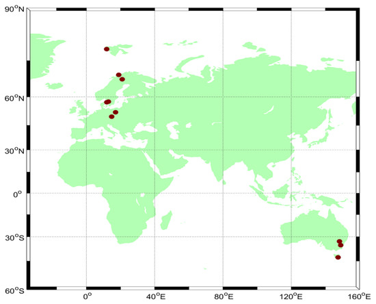
Figure 1.
Geographical distribution of collected stations in the experiment.

Table 1.
Information of utilized BDS stations in the experiment.
During the data processing, the precise time-transfer solution (PTTSol) was used [34]. The BDS satellite orbit and clock products from three IGS analysis centers, WUM, GFZ, and CODE, were employed for further research of the stability of ISBs when combining BDS-2 and BDS-3 for time transfer. The Wuhan University analysis center has provided BDS-3 satellite orbit and clock products since GPS week 2034, with 15 min and 5 min updates, using “wum” ID. GeoForschungsZentrum Potsdam has provided them since GPS week 2081, with 5 min and 30 s intervals, using “gbm” ID. Fortunately, starting from GPS week 2148, the CODE satellite solution has included BDS-3 (apart from GEO satellites), with a 5 min orbit and 30 s clock, using “com” ID. The pseudorange and CP measurements for B1, B3 of BDS-2, and BDS-3 dual-frequency observations are used to alleviate the ionosphere effect. In preprocessing, both the geometry-free combination and the Melbourne–Wübbena combination were used for cycle slip detection. Tropospheric wet delay is typically modeled as the sum of the Saastamoinen model and a random walk process. The receiver clock offset parameter was estimated as a white stochastic noise process. We also considered the wind-up effects on phase measurements. The data-processing strategies in this study are summarized in Table 2.
Table 2.
Data-processing strategies in this study.
4.1. Characterization of ISB over Different Time Periods
As the research was conducted over numerous days, we randomly selected the result on DOY 100, 110, and 120 of 2021 to analyze ISB variation. Figure 2 shows that the ISBs are stable with the different analysis center products on the three days. The average variation over the experimental period is within 0.08m for ISB_com and 0.07 m for ISB_gbm and ISB_wum. The variations on DOY 100 and 120 are within 0.06 m; however, the range on DOY 110 at 0.09 m is much larger than that for the other days. The difference between the minimum and maximum values is approximately 0.28 m for the ISB_com solution, 0.26 m for ISB_wum, and 0.25 m for ISB_gbm. Notably, the mean values of the results from three analysis centers differ markedly for one daily result. Figure 3 shows the mean value character of the results of different analysis centers of 10 stations. Although obvious systematic bias does exist among the com, gbm, and wum results, it is relatively stable among the ten stations. The systematic bias values between the com and wum results are −0.46 m, −0.50 m, and −0.33 m for DOY 100, 110, and 120, respectively, whereas for com and gbm the values are −1.65 m, −1.75 m, and −0.78 m, respectively, i.e., larger than the former. Systematic bias is caused mainly by the different data-processing strategies of the three analysis centers when determining the BDS-2 and BDS-3 satellite orbit and clock products. Figure 2 and Figure 3 show that the ISB trend is generally stable. The stability of ISB_gbm and ISB_wum is slightly superior to that of ISB_com. Remarkably, the mean value of the former four stations equipped with SEPT POLARX5 receivers is not more stable than that of the middle three stations (SEPT POLARX5TR) or the latter three stations (TRIMBLE NETR9). Relevant details on this aspect are presented in the following sections.
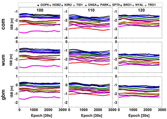
Figure 2.
Daily variations in ISB between BDS-3 and BDS-2 for 10 stations. The panels from top to bottom show the results of the com, wum, and gbm precise products.
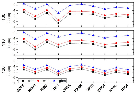
Figure 3.
Average of ISB between BDS-3 and BDS-2 for 10 stations for the com, wum, and gbm solutions.
4.2. Analysis of ISB for Different Station Attributes
From the Equation (10), we know that the ISB contains two components, the time difference of two receiver clock offsets with different GNSS observations, and the difference in the receiver hardware delays for two GNSS systems. For the latter, the receiver type, antenna, and frequency standard are the important factors to affect the receiver hardware delays. For further analyses of the relationship between the station attribute and ISB stability, the stations shown in Table 3 were regrouped into five comparative schemes according to three indicators, namely receiver type, antenna, and frequency standard. Table 3 shows the comparative strategies and corresponding stations, where ● means the same, and ○ means different. Further, to alleviate the effect of systematic bias in the results from different stations of three analysis centers on ISB stability analysis, the ISB difference of stations is more focused, which is also related to the calibration of the time-transfer links.
Table 3.
Comparative schemes and corresponding stations.
As 10 stations were involved in the 20 d experimental period, we randomly used the results of DOY 101, 106, 111, 115, and 119 of 2021 in the five comparison schemes, as shown in Figure 3, Figure 4, Figure 5, Figure 6 and Figure 7. To clearly plot and compare the receiver type, antennas, and frequency standards in the figures, we used abbreviations, namely “Rec”, “Ant”, and “Fre”.
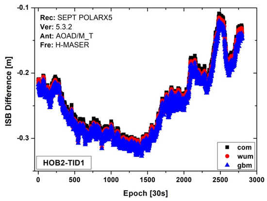
Figure 4.
ISB difference series for scheme 1 on DOY 101, 2021.
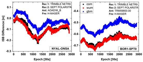
Figure 5.
ISB difference series for scheme 2 on DOY 106, 2021.
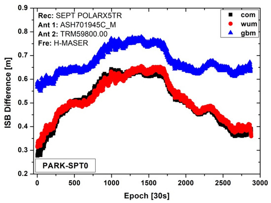
Figure 6.
ISB difference series for scheme 3 on DOY 111, 2021.
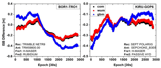
Figure 7.
ISB difference series for scheme 4 on DOY 115, 2021.
Figure 4 shows the ISB difference series for scheme 1, using the same receiver type, antenna, and frequency standard for SEPT POLARX5, AOAD/M_T, and H-MASER, respectively. One can see that the variation trends of ISB_com, ISB_wum, and ISB_gbm agree very well. The standard deviation (STD) values are all 0.05 m for the three analysis center products. The ranges between the minimum and maximum are 0.2 m.
Figure 5 shows the ISB difference series for scheme 2, which uses the same type of antenna and frequency standard, but different receiver types for one time-transfer link. The left panel shows the time link of station NYAL-ONSA, with the same type of antenna AOAD/M_B and frequency standard H-MASER. The right panel shows station BOR1-SPT0, with the same type of antenna TRM59800.00 and frequency standard H-MASER. The ISB difference series of and agree relatively well, whereas the difference series shows obvious bias compared with that of and for the two time-transfer links. The bias for NYAL-ONSA is approximately 0.07 m and that for BOR1-SPT0 is approximately 0.12 m. The standard deviation of divergence is approximately 0.014 m and 0.013 m, respectively. The above analyses show that the ISB difference series has a close relationship with the type of receiver of the different analysis center products.
Figure 6 shows the ISB difference series for scheme 3, which uses the same type of receiver and frequency standard, but a different antenna type. This scheme is similar to scheme 2, and the difference series of and show good agreement, although the antenna type differs. Obvious bias exists between , , and , with the corresponding values ranging from 0.1 m to 0.25 m. This finding indicates that the ISB difference series has a certain relationship with the antenna type for the three analysis centers’ satellite orbits and clock products. Compared with , the mean value of divergence is 0.010 m for and 0.167 m for , and the standard deviations are 0.013 m and 0.050 m.
Figure 7 shows the ISB difference series for scheme 4, which uses the same type of receiver and antenna, but a different frequency standard. The left panel is the time link of station BOR1-TRO1, with the same type of receiver TRIMBLE NETR9 and antenna TRM59800.00. The right panel is station KIRU-GOP6, with the same type of receiver SEPT POLARX5 and antenna SEPCHOKE_B3E6. The variations in the ISB difference series for the and solutions are in extremely good agreement. Although the general trend of is somewhat similar, the divergence between and the former two solutions does not show constant bias, but indicates significant variation for the two time-transfer links.
Figure 8 shows the ISB difference series for scheme 5, which uses different receivers, antennas, and frequency standards. Although the general trend is somewhat similar, the divergence among ISB_com, ISB_wum, and ISB_gbm shows not only obvious bias but also the variation term. As indicated by the analyses and discussions of the five schemes, the ISB difference of ISB_com and ISB_wum agrees well. The mean value of divergence is 0.023 m for ISB_wum and 0.030 m for ISB_gbm, and the standard deviations are 0.030 m and 0.036 m compared with those of ISB_com.
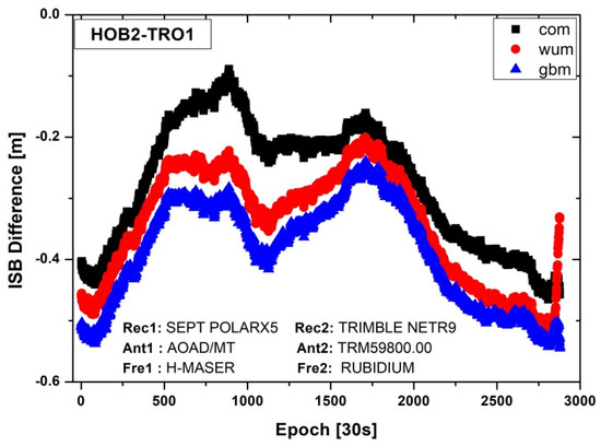
Figure 8.
ISB difference series for scheme 5 on DOY 119, 2021.
4.3. Influence of Different ISB Stochastic Models on Time and Frequency Transfer
To assess the characteristics of different ISB stochastic models in the time and frequency transfer, the previous three modes are applied in the experiment. Then, the ISB were modeled as constants for one hour in a model of random constant process, marked as “constant.” For the random walk process, it was defined as “walk” and the power density was 1 mm/s0.5, whereas the white noise process was marked as “noise.” Figure 9 shows the results of time and frequency with three ISB stochastic models on the time link PTBB–WTZZ, using GFZ precise products. The variations in the clock difference agree well for the three ISB stochastic models. Figure 10 shows a comparison of Allan deviations of time-transfer results for the three ISB stochastic models at the PTBB–WTZZ time link. It is clear that the “constant” and “walk” schemes show slightly superior performances for frequency stability compared with that of “noise” at different time intervals. The average values within 10,000 s among the solutions of the three models are 1.08 × 10⁻¹³ for “noise”, 1.00 × 10⁻¹³ for “constant,” and 9.95 × 10⁻¹³ for “walk,” with the improvements being 5.08% and 5.67%, respectively.
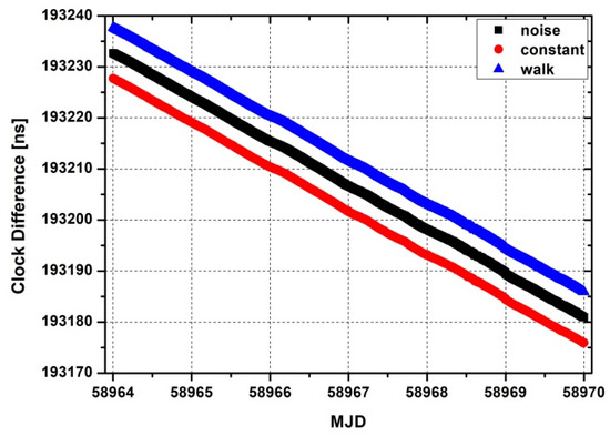
Figure 9.
Result of time and frequency transfer with three ISB stochastic models on time link PTBB–WTZZ. For plotting purposes, the overall values for “walk” results were translated up to 5 ns, whereas those for results using the constant were translated down to 5 ns.
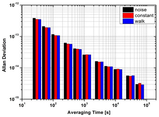
Figure 10.
Comparison of Allan deviations in time-transfer results for the three ISB stochastic models at the PTBB–WTZZ time link.
5. Discussion
The multi-GNSS time and frequency transfer is essential for UTC comparison and traceability services, particularly for the existing BDS-2 regional and BDS-3 global system. However, the character of intersystem biases in the BDS-2/BDS-3 GNSS time and frequency transfer is still unclear. Therefore, the spatiotemporal characterization, different station attributes, and stochastic models of ISB were focused.
One can note that the daily ISB in BDS-2/BDS-3 is relatively stable, but exhibits obvious discrepancies among the three IGS analysis centers. Considering that the current BDS daily products have an obvious day-boundary jump, the daily stability of ISB helps to precisely estimate parameters. From the results of ISB for different station attributes, it can be see that common receiver type, antenna, and frequency standard can contribute to improving consistency for the three different analysis centers, these mainly being caused by the relationship between the attribute of the station (receiver DCB [35], receiver calibration, type of frequency standard) and the strategies of satellite products (i.e., sample interval, data-processing strategy, used stations, and so on). In addition, the three ISB stochastic models are compared in the time and frequency transfer, which agree with the results in previous research [32].
Of course, this study proposes only the first step of this research, and several topics still require further investigation in our near future work; for example, how to use a functional model to improve the estimation precision of ISB, and how to calibrate the ISB delay in the time link based on multisystem time and frequency transfer.
6. Conclusions
To maintain the consistency and continuity from BDS-2 to BDS-3 time transfer for one time link, we analyzed the ISBs in BDS-2/BDS-3. We deduced the mathematical model of BDS-2/BDS-3 time and frequency transfer, including observation and stochastic models. The temporal characteristics of ISB for different types of receivers, antennas, and frequency standards, with different IGS analysis center products were discussed. The three stochastic models of ISB were evaluated using one time link.
Our results indicated that the ISB series exhibit obvious discrepancies among the three analysis centers, but relatively stable characteristics. The mean values of the daily results of differ markedly for the three analysis centers. The receiver type, antenna, and frequency standard have a certain influence on the ISB difference in time and frequency transfer. The receiver type, antenna, and frequency standard are different for the two ends of the time link; the obvious system bias exists among the com, gbm, and wum analysis centers. As the only different receiver type scheme, the ISB difference series of ISB_com and ISB_wum agree relatively well, whereas the ISB_gbm series shows obvious bias compared with ISB_com and ISB_wum for the two time-transfer links. The bias differs for the two time links. The bias for station NYAL-ONSA is approximately 0.07 m, and that for station BOR1-SPT0 is approximately 0.12 m. The ISB difference series of ISB_com and ISB_wum agree relatively well for the only different antenna type scheme, whereas the ISB_gbm series shows obvious bias compared with ISB_com and ISB_wum for the two time-transfer links. It should be noted that the bias is not a constant but varies with time. As the only different-frequency-standard scheme, the general trend of ISB_gbm is somewhat similar; the divergence between ISB_wum and the other two solutions is not constant but shows significant variations for the two time-transfer links. The effect of the three different ISB stochastic models was assessed with respect to time and frequency transfer. The “walk” and “constant” schemes were slightly superior to the “noise”, with the improvements in frequency stability being approximately 5.08% and 5.67%, respectively, compared with that of “noise”.
This study proposes only the first step of this research, and several topics still require further investigation in our near-future work; for example, how to use a functional model to improve the estimation precision of ISB, and how to calibrate the ISB delay in the time link based on multisystem time and frequency transfer.
Author Contributions
P.Z. and R.T. conceived and designed the experiments; P.Z. performed the experiments, analyzed the data and wrote the paper. L.T., B.W., Y.G. and X.L. contributed to discussions and revisions. All authors have read and agreed to the published version of the manuscript.
Funding
This research was funded by National Natural Science Foundation of China (Grant No: 11903040, 41674034, 41974032, 42030105) and Chinese Academy of Sciences (CAS) programs of “Youth Innovation Promotion Association” (Grant No: 2022414), “Western young scholars” (Grant No.: XAB2019B21), China Postdoctoral Science Foundation (Grant No: 2020M683763).
Data Availability Statement
The datasets analyzed in this study are managed by the MGEX and National Time Service Center, Chinese Academy of Sciences, which can be available on request from the corresponding author.
Acknowledgments
Many thanks go to the IGS MGEX for providing multi-GNSS ground tracking data, precise orbit, and clock products.
Conflicts of Interest
The authors declare no conflict of interest.
References
- Wang, M.; Wang, J.; Dong, D.; Meng, L.; Chen, J.; Wang, A.; Cui, H. Performance of BDS-3: Satellite visibility and dilution of precision. GPS Solut. 2019, 23, 56. [Google Scholar] [CrossRef]
- Yang, Y.; Mao, Y.; Sun, B. Basic performance and future developments of BeiDou global navigation satellite system. Satell. Navig. 2020, 1, 1. [Google Scholar] [CrossRef]
- Yang, Y.; Gao, W.; Guo, S.; Mao, Y.; Yang, Y. Introduction to BeiDou-3 navigation satellite system. Navigation 2019, 66, 7–18. [Google Scholar] [CrossRef]
- Mi, X.; Sheng, C.; El-Mowafy, A.; Zhang, B. Characteristics of receiver-related biases between BDS-3 and BDS-2 for five frequencies including inter-system biases, differential code biases, and differential phase biases. GPS Solut. 2021, 25, 113. [Google Scholar] [CrossRef]
- Harmegnies, A.; Defraigne, P.; Petit, G. Combining GPS and GLONASS in all-in-view for time transfer. Metrologia 2013, 50, 277–287. [Google Scholar] [CrossRef]
- Zhang, P.; Tu, R.; Gao, Y.; Zhang, R.; Liu, N. Improving the Performance of Multi-GNSS Time and Frequency Transfer Using Robust Helmert Variance Component Estimation. Sensors 2018, 18, 2878. [Google Scholar] [CrossRef] [PubMed]
- Dow, J.; Neilan, R.; Rizos, C. The International GNSS Service in a changing landscape of Global Navigation Satellite Systems. J. Geod. 2009, 83, 191–198. [Google Scholar] [CrossRef]
- Montenbruck, O.; Steigenberger, P.; Prange, L.; Deng, Z.; Zhao, Q.; Perosanz, F.; Schaer, S. The Multi-GNSS Experiment (MGEX) of the International GNSS Service (IGS)–Achievements, prospects and challenges. Adv. Sp. Res. 2017, 59, 1671–1697. [Google Scholar] [CrossRef]
- Li, X.; Ge, M.; Dai, X.; Ren, X.; Fritsche, M.; Wickert, J.; Schuh, H. Accuracy and reliability of multi-GNSS real-time precise positioning: GPS, GLONASS, BeiDou, and Galileo. J. Geod. 2015, 89, 607–635. [Google Scholar] [CrossRef]
- Jin, S.; Wang, Q.; Dardanelli, G. A Review on Multi-GNSS for Earth Observation and Emerging Applications. Remote Sens. 2022, 14, 3930. [Google Scholar] [CrossRef]
- Jiang, Z.; Lewandowski, W. Use of GLONASS for UTC time transfer. Metrologia 2012, 49, 57–61. [Google Scholar] [CrossRef]
- Petit, G.; Defraigne, P. The performance of GPS time and frequency transfer: Comment on A detailed comparison of two continuous GPS carrier-phase time transfer techniques. Metrologia 2016, 53, 1003–1008. [Google Scholar] [CrossRef]
- Yi, H.; Wang, H.; Zhang, S.; Wang, H.; Shi, F.; Wang, X. Remote time and frequency transfer experiment based on BeiDou Common View. In Proceedings of the European Frequency and Time Forum (EFTF), York, UK, 26 May 2016; pp. 1–4. [Google Scholar] [CrossRef]
- Guang, W.; Dong, S.; Wu, W.; Zhang, J.; Yuan, Y.; Zhang, S. Progress of BeiDou time transfer at NTSC. Metrologia 2018, 55, 175–187. [Google Scholar] [CrossRef]
- Wu, M.; Liu, W.; Wang, W.; Zhang, X. Differential Inter-System Biases Estimation and Initial Assessment of Instantaneous Tightly Combined RTK with BDS-3, GPS, and Galileo. Remote Sens. 2019, 11, 1430. [Google Scholar] [CrossRef]
- Defraigne, P.; Aerts, W.; Harmegnies, A.; Petit, G.; Rovera, D.; Uhrich, P. Advances in multi-GNSS time transfer. In Proceedings of the European Frequency and Time Forum and International Frequency Control Symposium, Prague, Czech Republic, 21–25 July 2013; pp. 508–512. [Google Scholar]
- Li, X.; Xie, W.; Huang, J.; Ma, T.; Zhang, X.; Yuan, Y. Estimation and analysis of differential code biases for BDS3/BDS2 using iGMAS and MGEX observations. J. Geod. 2019, 93, 419–435. [Google Scholar] [CrossRef]
- Pan, L.; Zhang, Z.; Yu, W.; Dai, W. Intersystem Bias in GPS, GLONASS, Galileo, BDS-3, and BDS-2 Integrated SPP: Characteristics and Performance Enhancement as a Priori Constraints. Remote Sens. 2021, 13, 4650. [Google Scholar] [CrossRef]
- Zhao, W.; Chen, H.; Gao, Y.; Jiang, W.; Liu, X. Evaluation of Inter-System Bias between BDS-2 and BDS-3 Satellites and Its Impact on Precise Point Positioning. Remote Sens. 2020, 12, 2185. [Google Scholar] [CrossRef]
- Fu, W.; Wang, L.; Li, T.; Chen, R.; Han, Y.; Zhou, H.; Li, T. Combined BDS-2/BDS-3 real-time satellite clock estimation with the overlapping B1I/B3I signals. Adv. Sp. Res. 2021, 66, 4470–4483. [Google Scholar] [CrossRef]
- Dai, P.; Yang, X.; Qin, W.; Wang, R.; Zhang, Z. Analysis of BDS-2+BDS-3 Combination Real-Time Time Transfer Based on iGMAS Station. In Proceedings of the 10th China Satellite Navigation Conference (CSNC), Beijing, China, 22–25 May 2019. [Google Scholar]
- Su, K.; Jin, S. Triple-frequency carrier phase precise time and frequency transfer models for BDS-3. GPS Solut. 2019, 23, 86. [Google Scholar] [CrossRef]
- Zhang, P.; Tu, R.; Zhang, R.; Liu, N.; Gao, Y. Time and frequency transfer using BDS-2 and BDS-3 carrier-phase observations. IET Radar Sonar Navig. 2019, 13, 1249–1255. [Google Scholar] [CrossRef]
- Jiao, G.; Song, S.; Chen, Q.; Huang, C.; Su, K.; Wang, Z.; Cheng, N. Modeling and Analysis of BDS-2 and BDS-3 Combined Precise Time and Frequency Transfer Considering Stochastic Models of Inter-System Bias. Remote Sens. 2021, 13, 793. [Google Scholar] [CrossRef]
- Gong, X.; Zheng, F.; Gu, S.; Zheng, F.; Lou, Y. The long-term characteristics of GNSS signal distortion biases and their empirical corrections. GPS Solut. 2022, 26, 52. [Google Scholar] [CrossRef]
- Nicolini, L.; Caporali, A. Investigation on Reference Frames and Time Systems in Multi-GNSS. Remote Sens. 2018, 10, 80. [Google Scholar] [CrossRef]
- Defraigne, P.; Baire, Q. Combining GPS and GLONASS for time and frequency transfer. Adv. Space Res. 2011, 47, 265–275. [Google Scholar] [CrossRef]
- Gong, X.; Gu, S.; Lou, Y.; Zheng, F.; Yang, X.; Wang, Z.; Liu, J. Research on empirical correction models of GPS Block IIF and BDS satellite inter-frequency clock bias. J. Geod. 2020, 94, 36. [Google Scholar] [CrossRef]
- Rovera, G.D.; Torre, J.M.; Sherwood, R.; Abgrall, M.; Courde, C.; Laas-Bourez, M.; Uhrich, P. Link calibration against receiver calibration: An assessment of GPS time transfer uncertainties. Metrologia 2014, 51, 476–490. [Google Scholar] [CrossRef]
- Zhang, P.; Tu, R.; Gao, Y.; Guang, W.; Zhang, R.; Cai, H. Study of time link calibration based on GPS carrier phase observation. IET Radar Sonar Navig. 2018, 12, 1330–1335. [Google Scholar] [CrossRef]
- Lou, Y.; Gong, X.; Gu, S.; Zheng, F.; Feng, Y. Assessment of code bias variations of BDS triple-frequency signals and their impacts on ambiguity resolution for long baselines. GPS Solut. 2017, 21, 177–186. [Google Scholar] [CrossRef]
- Zhang, P.; Tu, R.; Han, J.; Zhang, R.; Gao, Y.; Lu, X. Characterization of biases between BDS-3 and BDS-2, GPS, Galileo and GLONASS observations and their effect on precise time and frequency transfer. Meas. Sci. Technol. 2021, 32, 035006. [Google Scholar] [CrossRef]
- Zhou, F.; Dong, D.; Li, P.; Li, X.; Schuh, H. Influence of stochastic modeling for inter-system biases on multi-GNSS undifferenced and uncombined precise point positioning. GPS Solut. 2019, 23, 59. [Google Scholar] [CrossRef]
- Zhang, P.; Tu, R.; Zhang, R.; Gao, Y.; Cai, H. Combining GPS, BeiDou, and Galileo Satellite Systems for Time and Frequency Transfer Based on Carrier Phase Observations. Remote Sens. 2018, 10, 324. [Google Scholar] [CrossRef]
- Choi, B.; Lee, S. The influence of grounding on GPS receiver differential code biases. Adv. Sp. Res. 2018, 62, 457–463. [Google Scholar] [CrossRef]
Publisher’s Note: MDPI stays neutral with regard to jurisdictional claims in published maps and institutional affiliations. |
© 2022 by the authors. Licensee MDPI, Basel, Switzerland. This article is an open access article distributed under the terms and conditions of the Creative Commons Attribution (CC BY) license (https://creativecommons.org/licenses/by/4.0/).