

Assessment of Real-Time GPS/BDS-2/BDS-3 Single-Frequency PPP and INS Tight Integration Using Different RTS Products

Abstract
:1. Introduction
2. Methodology
2.1. Real-Time SF-PPP Model
2.2. GPS/BDS-2/BDS-3 SF-PPP/INS Tight Integration Model
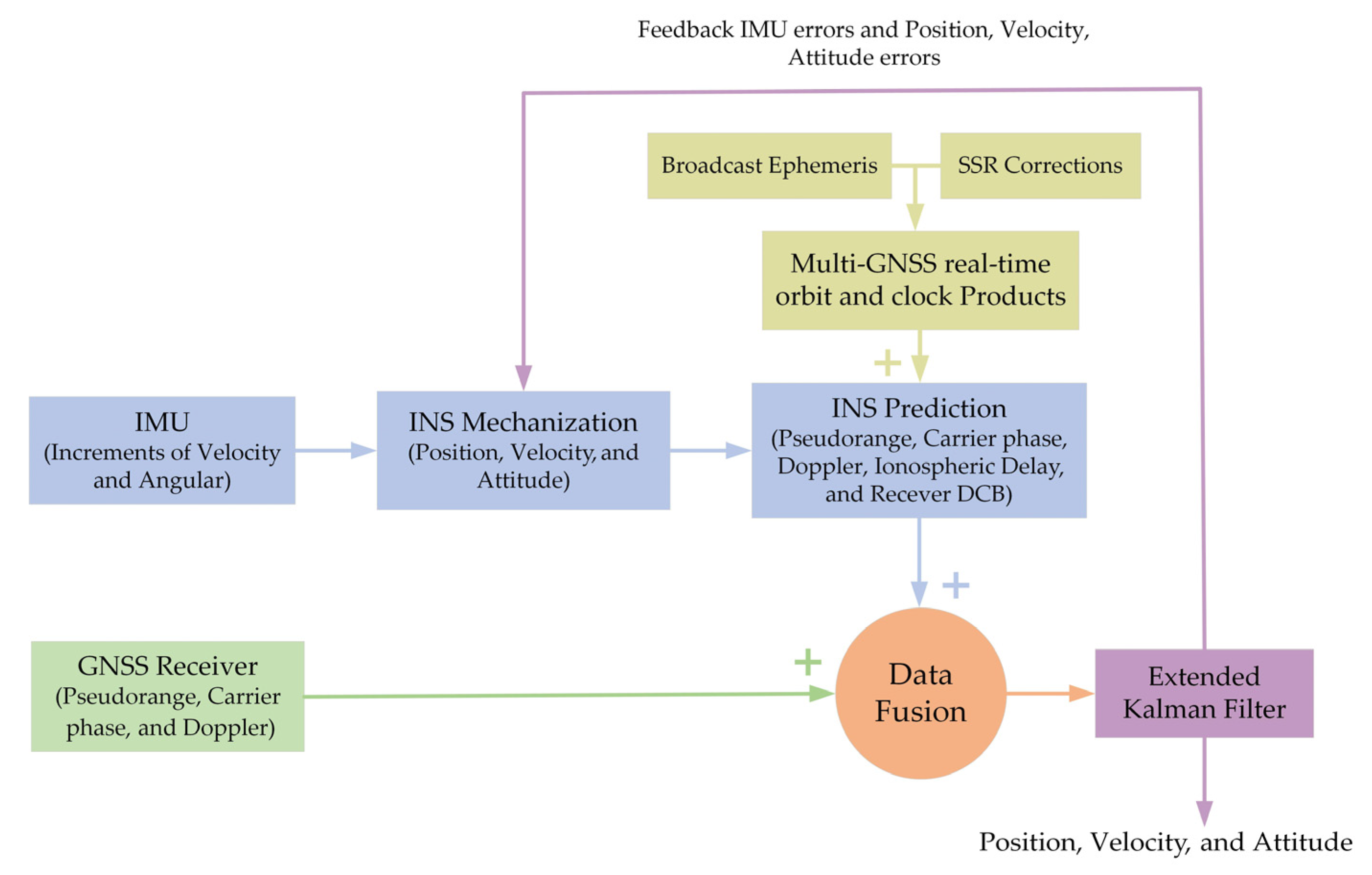
2.3. Implementation of SF-PPP/INS Tight Integration Model
3. Tests, Results, and Discussions
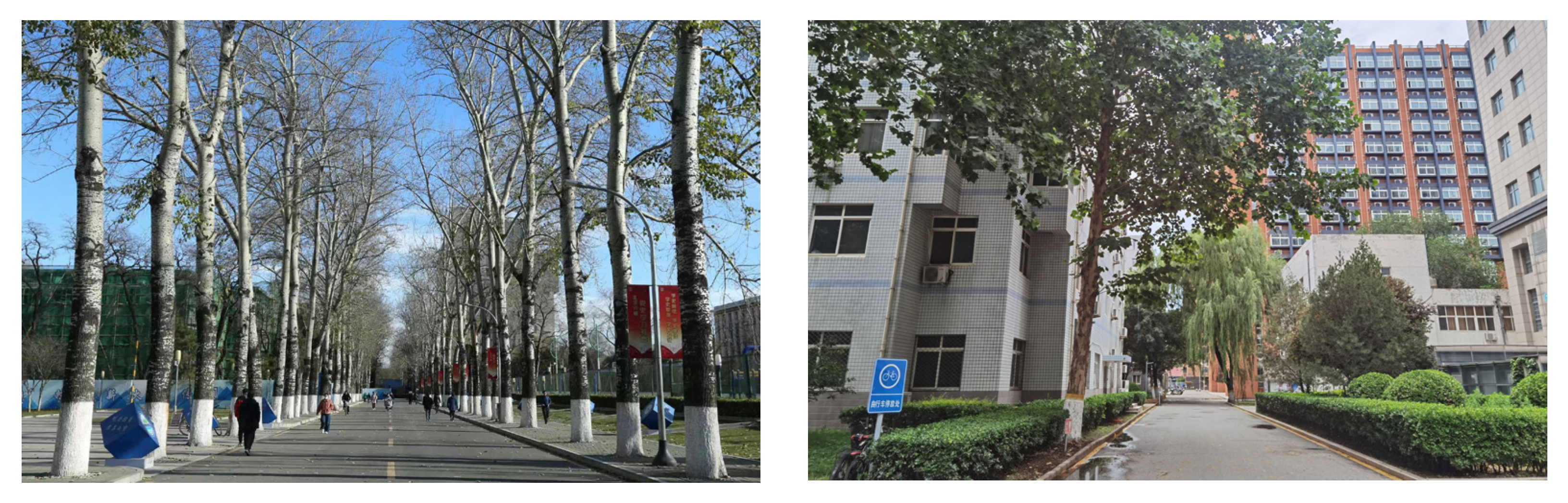
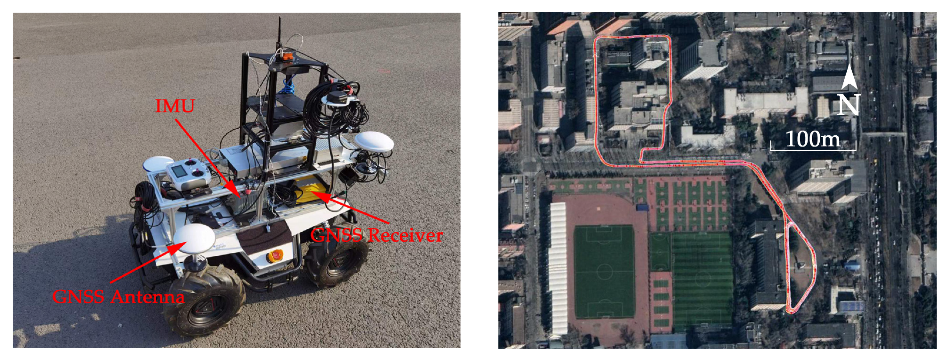
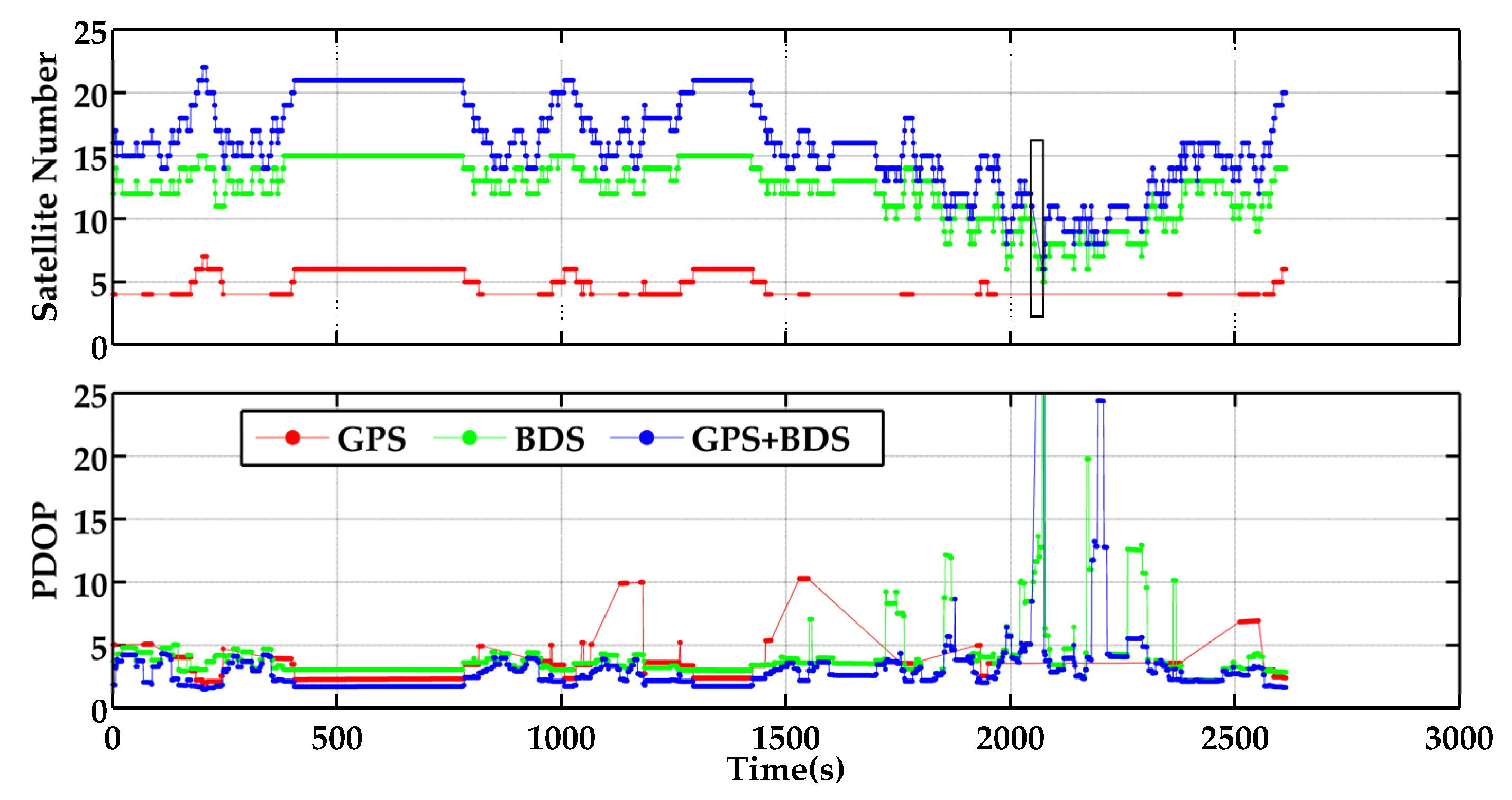
3.1. Data Collection
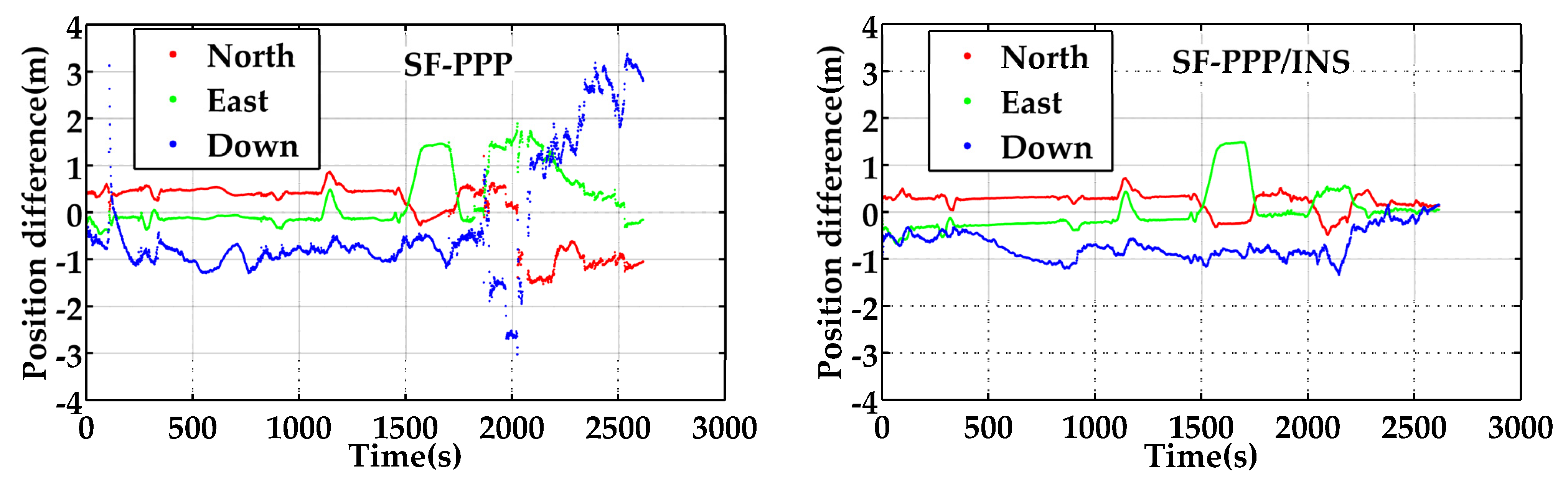
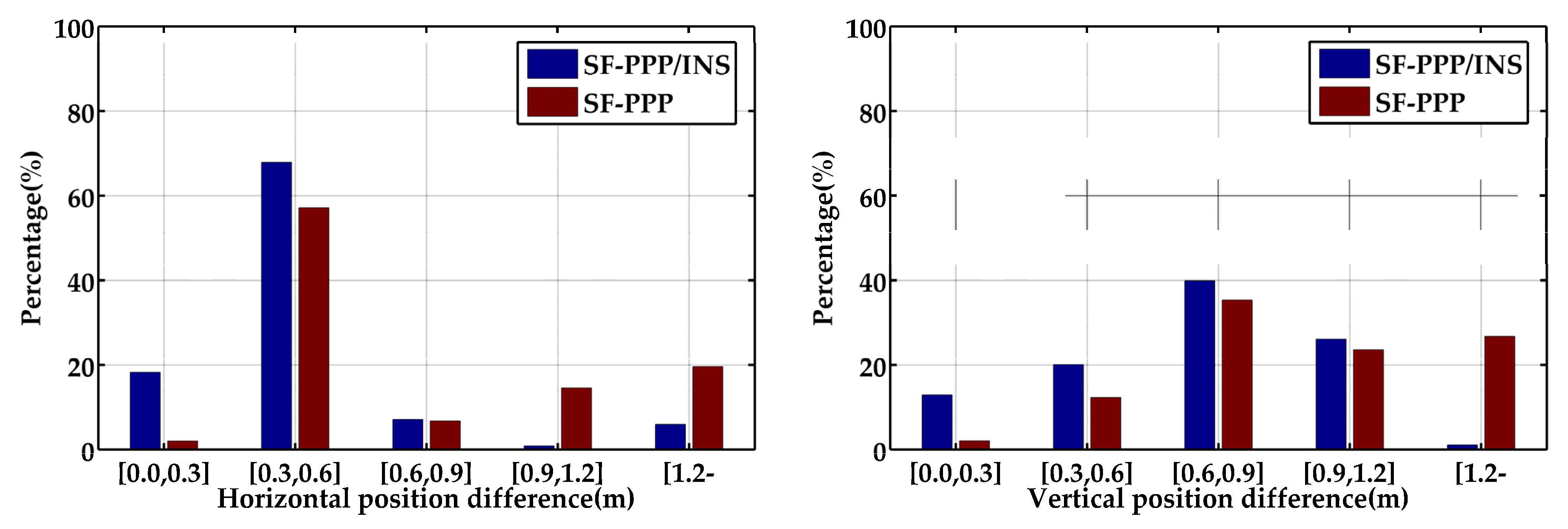
3.2. Positioning Performance of PPP and PPP/INS Tight Integration
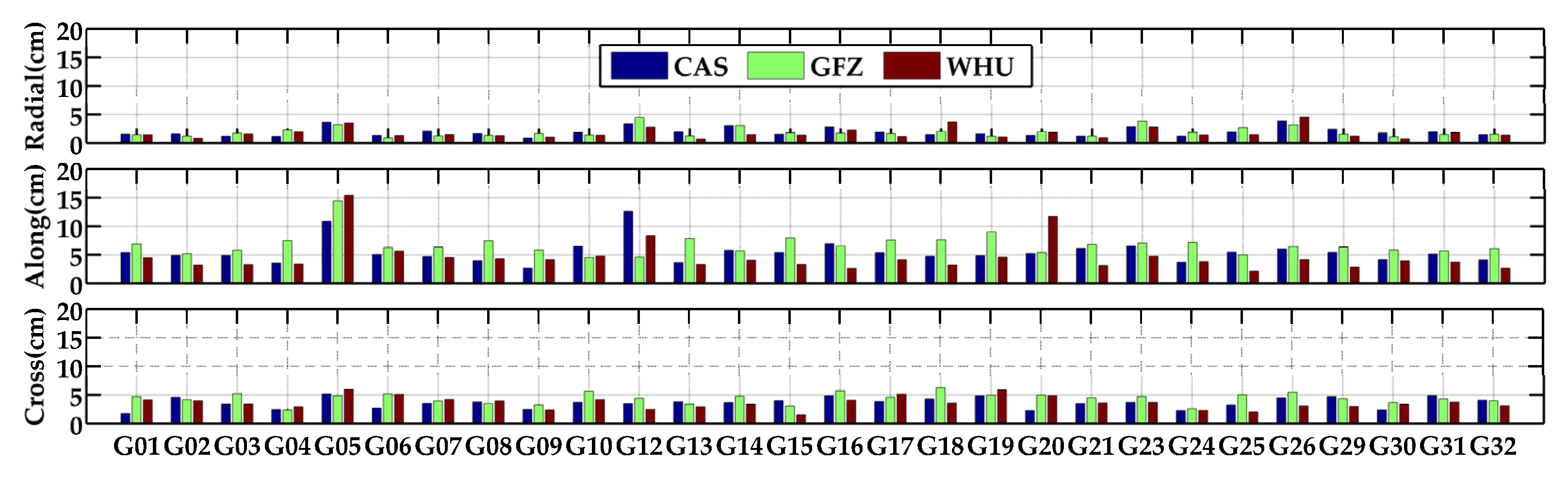
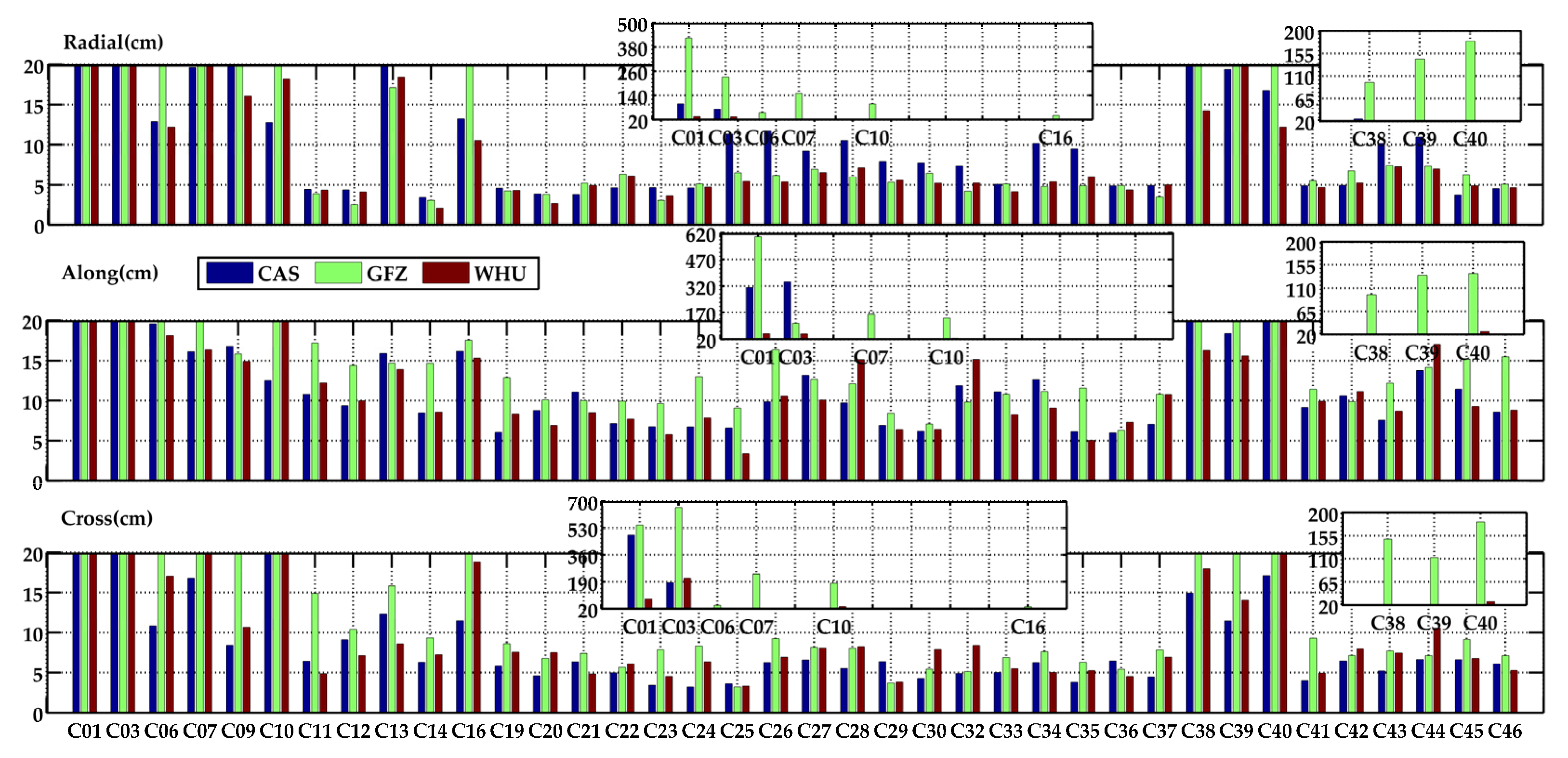
3.3. Evaluation of Real-Time Orbit and Clock Products
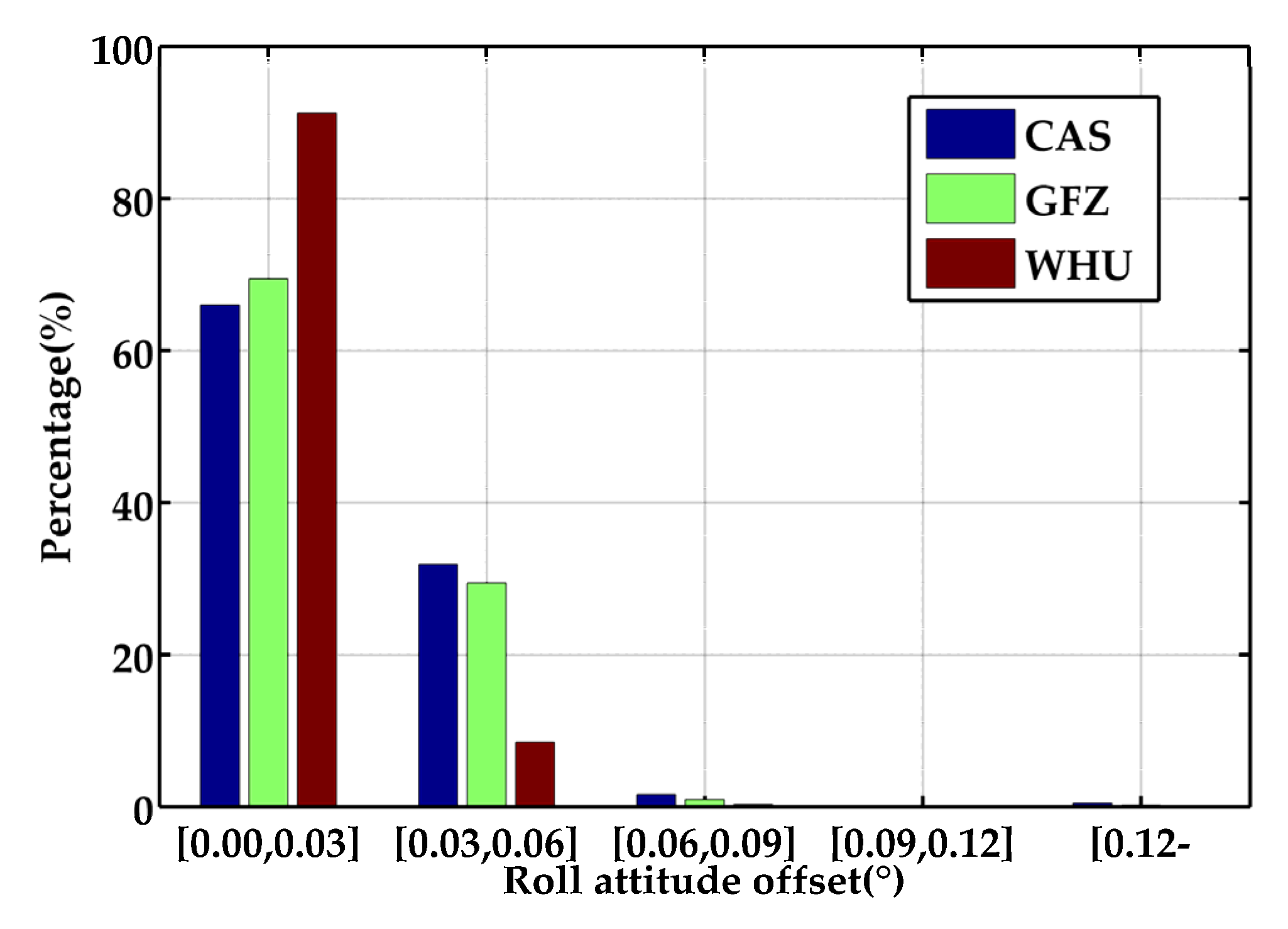
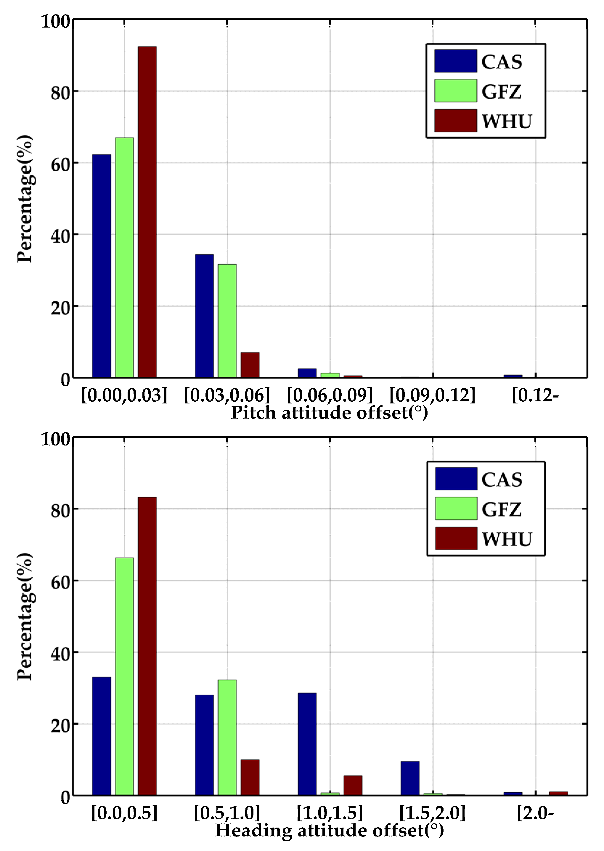
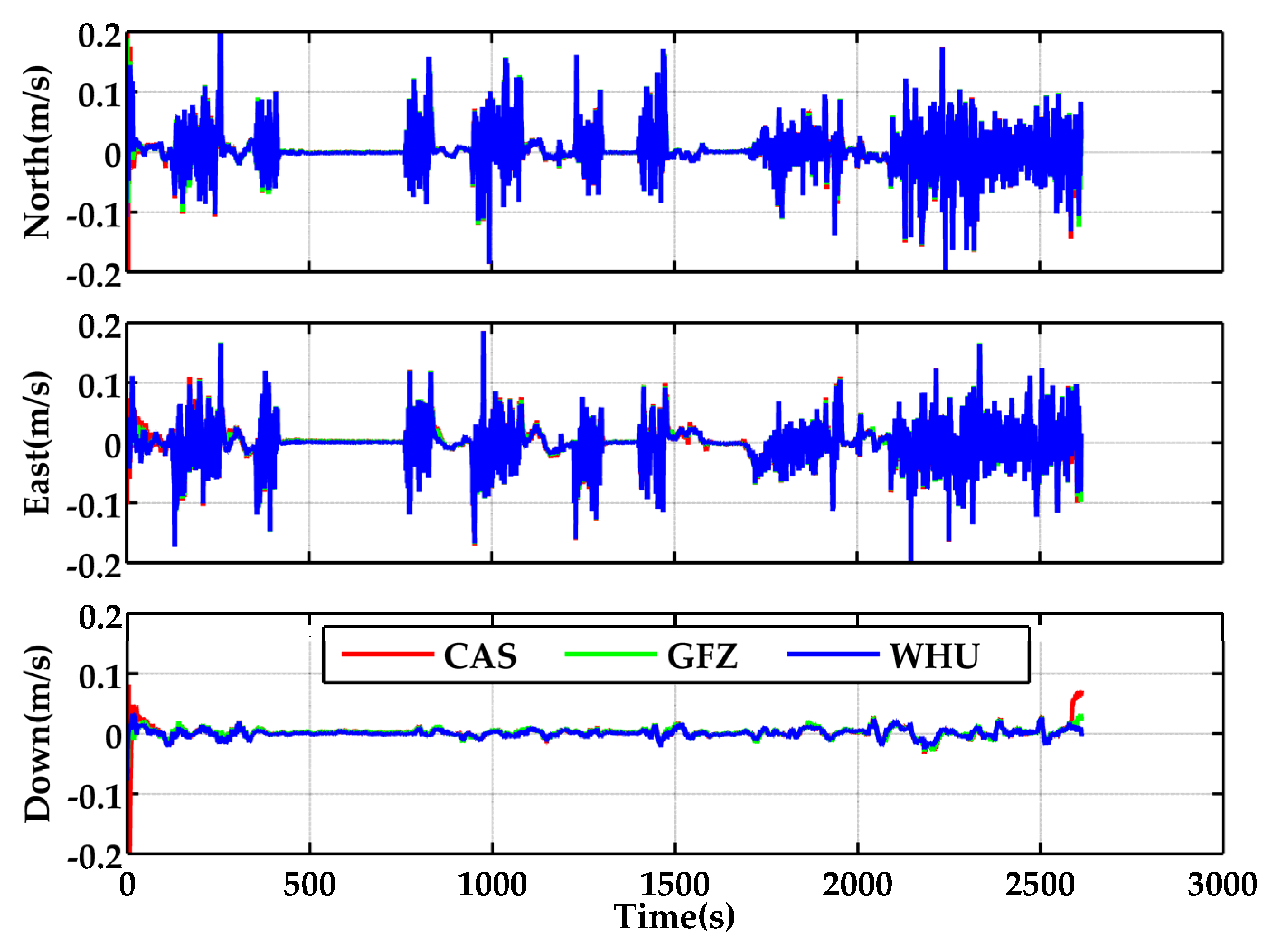
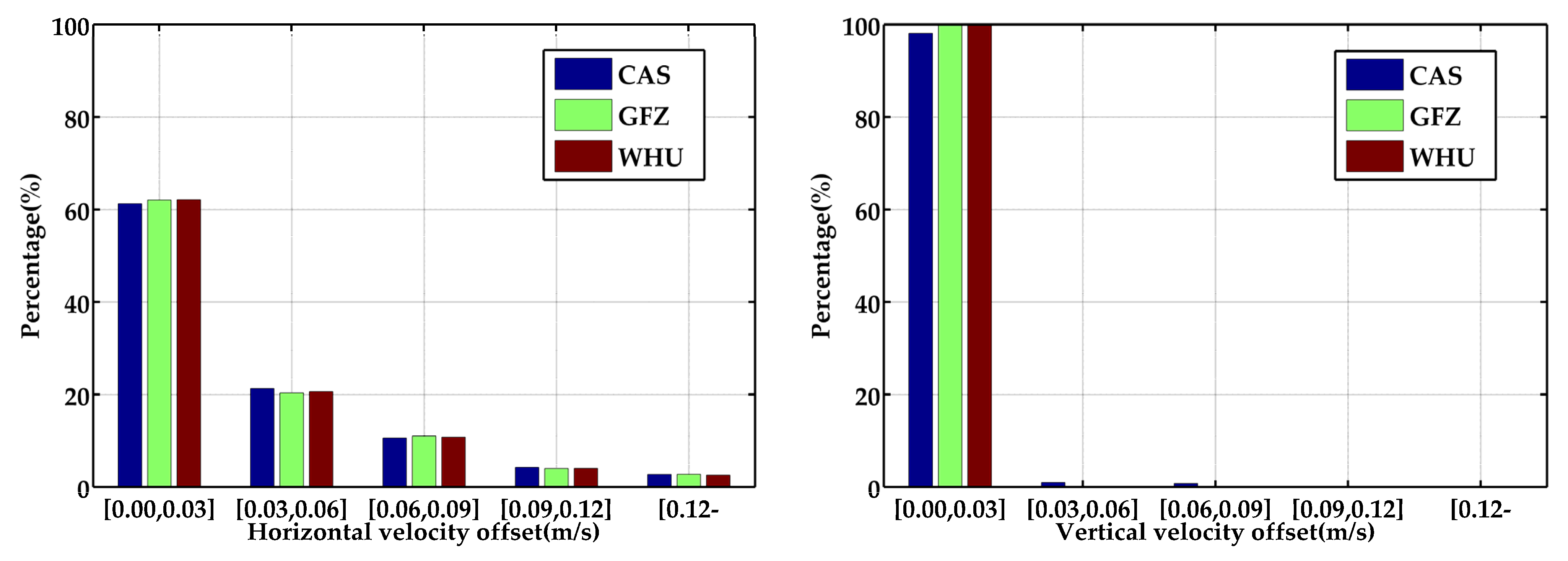
3.4. Performance of Real-Time PPP/INS Tight Integration
4. Conclusions
Author Contributions
Funding
Data Availability Statement
Acknowledgments
Conflicts of Interest
References
- Zumberge, J.F.; Heflin, M.B.; Jefferson, D.C.; Watkins, M.M.; Webb, F.H. Precise point positioning for the efficient and robust analysis of GPS data from large networks. J. Geophys. Res. Solid Earth 1997, 102, 5005–5017. [Google Scholar] [CrossRef]
- Malys, S.; Jensen, P.A. Geodetic point positioning with GPS carrier beat phase data from the CASA UNO experiment. Geophys. Res. Lett. 1990, 17, 651–654. [Google Scholar] [CrossRef]
- Larson, K.M.; Bodin, P.; Gomberg, J. Using 1-Hz GPS data to measure deformations caused by the Denali fault earthquake. Science 2003, 300, 1421–1424. [Google Scholar] [CrossRef] [PubMed]
- Li, X.; Ge, M.; Lu, C.; Zhang, Y.; Wang, R.; Wickert, J.; Schuh, H. High-Rate GPS Seismology Using Real-Time Precise Point Positioning with Ambiguity Resolution. IEEE Trans. Geosci. Remote Sens. 2014, 52, 6165–6180. [Google Scholar]
- Yao, Y.; Liu, C.; Xu, C. A New GNSS-Derived Water Vapor Tomography Method Based on Optimized Voxel for Large GNSS Network. Remote Sens. 2020, 12, 2306. [Google Scholar] [CrossRef]
- Li, X.; Zhang, X.; Guo, F. Predicting atmospheric delays for rapid ambiguity resolution in precise point positioning. Adv. Space Res. 2014, 54, 840–850. [Google Scholar] [CrossRef]
- Zhang, K.; Liang, S.; Gan, W. Crustal strain rates of southeastern Tibetan Plateau derived from GPS measurements and implications to lithospheric deformation of the Shan-Thai terrane. Earth Planet. Phys. 2019, 3, 45–52. [Google Scholar] [CrossRef]
- Zhang, K.; Wang, Y.; Gan, W.; Liang, S. Impacts of Local Effects and Surface Loads on the Common Mode Error Filtering in Continuous GPS Measurements in the Northwest of Yunnan Province, China. Sensors 2020, 20, 5408. [Google Scholar] [CrossRef]
- Lou, Y.; Zheng, F.; Gu, S.; Wang, C.; Guo, H.; Feng, Y. Multi-GNSS precise point positioning with raw single-frequency and dual-frequency measurement models. GPS Solut. 2016, 20, 849–862. [Google Scholar] [CrossRef]
- Ge, Y.; Dai, P.; Qin, W.; Yang, X.; Zhou, F.; Wang, S.; Zhao, X. Performance of Multi-GNSS Precise Point Positioning Time and Frequency Transfer with Clock Modeling. Remote Sens. 2019, 11, 347. [Google Scholar] [CrossRef]
- Lv, J.; Gao, Z.; Kan, J.; Lan, R.; Li, Y.; Lou, Y.; Yang, H.; Peng, J. Modeling and assessment of multi-frequency GPS/BDS-2/BDS-3 kinematic precise point positioning based on vehicle-borne data. Measurement 2022, 189, 110453. [Google Scholar] [CrossRef]
- Li, X.; Li, X.; Ma, F.; Yuan, Y.; Zhang, K.; Zhou, F.; Zhang, X. Improved PPP Ambiguity Resolution with the Assistance of Multiple LEO Constellations and Signals. Remote Sens. 2019, 11, 408. [Google Scholar] [CrossRef]
- Geng, J.; Meng, X.; Dodson, A.H.; Ge, M.; Teferle, F.N. Rapid re-convergences to ambiguity-fixed solutions in precise point positioning. J. Geod. 2010, 84, 705–714. [Google Scholar] [CrossRef]
- Zhang, H.; Gao, Z.; Ge, M.; Niu, X.; Huang, L.; Tu, R.; Li, X. On the convergence of ionospheric constrained precise point positioning (IC-PPP) based on undifferential uncombined raw GNSS observations. Sensors 2013, 13, 15708–15725. [Google Scholar] [CrossRef]
- Zhang, B.; Teunissen, P.J.G.; Yuan, Y.; Zhang, X.; Li, M. A modified carrier-to-code leveling method for retrieving ionospheric observables and detecting short-term temporal variability of receiver differential code biases. J. Geod. 2019, 93, 19–28. [Google Scholar] [CrossRef]
- Guo, F.; Zhang, X.; Wang, J.; Ren, X. Modeling and assessment of triple-frequency BDS precise point positioning. J. Geod. 2016, 90, 1223–1235. [Google Scholar] [CrossRef]
- Hong, J.; Tu, R.; Zhang, R.; Fan, L.; Zhang, P.; Han, J. Contribution analysis of QZSS to single-frequency PPP of GPS/BDS/GLONASS/Galileo. Adv. Space Res. 2020, 65, 1803–1817. [Google Scholar] [CrossRef]
- Shi, C.; Wu, X.; Zheng, F.; Wang, X.; Wang, J. Modeling of BDS-2/BDS-3 single-frequency PPP with B1I and B1C signals and positioning performance analysis. Measurement 2021, 178, 109355. [Google Scholar] [CrossRef]
- Su, K.; Jin, S. A novel GNSS single-frequency PPP approach to estimate the ionospheric TEC and satellite pseudorange observable-specific signal bias. IEEE Trans. Geosci. Remote Sens. 2022, 60, 5801712. [Google Scholar] [CrossRef]
- Cox, D.B. Integration of GPS with Inertial Navigation Systems. Navig. J. Inst. Navig. 1978, 25, 236–245. [Google Scholar] [CrossRef]
- Gao, Z.; Ge, M.; Shen, W.; Zhang, H.; Niu, X. Ionospheric and receiver DCB-constrained multi-GNSS single-frequency PPP integrated with MEMS inertial measurements. J. Geod. 2017, 91, 1351–1366. [Google Scholar] [CrossRef]
- Gu, S.; Dai, C.; Fang, W.; Zheng, F.; Wang, Y.; Zhang, Q.; Lou, Y.; Niu, X. Multi-GNSS PPP/INS tightly coupled integration with atmospheric augmentation and its application in urban vehicle navigation. J. Geod. 2021, 95, 1–15. [Google Scholar] [CrossRef]
- Hadas, T.; Bosy, J. IGS RTS precise orbits and clocks verification and quality degradation over time. GPS Solut. 2015, 19, 93–105. [Google Scholar] [CrossRef]
- Wang, L.; Li, Z.; Ge, M.; Neitzel, F.; Wang, X.; Yuan, H. Investigation of the performance of real-time BDS-only precise point positioning using the IGS real-time service. GPS Solut. 2019, 23, 1–12. [Google Scholar] [CrossRef]
- Kazmierski, K.; Zajdel, R.; Sośnica, K. Evolution of orbit and clock quality for real-time multi-GNSS solutions. GPS Solut. 2020, 24, 1–12. [Google Scholar] [CrossRef]
- Øvstedal, O. Absolute positioning with single-frequency GPS receivers. GPS Solut. 2002, 5, 33–44. [Google Scholar] [CrossRef]
- Yunck, T.P. Orbit determination. In Global Positioning System-Theory and Applications; Parkinson, B.W., Spilker, J.J., Eds.; AIAA: Washington, DC, USA, 1996. [Google Scholar]
- Beran, T.; Kim, D.; Langley, R.B. High-precision single-frequency GPS point positioning. In Proceedings of the 16th International Technical Meeting of the Satellite Division of The Institute of Navigation (ION GPS/GNSS 2003), Portland, OR, USA, 9–12 September 2003; pp. 1192–1200. [Google Scholar]
- Montenbruck, O. Kinematic GPS positioning of LEO satellites using ionosphere-free single frequency measurements. Aerosp. Sci. Technol. 2003, 7, 396–405. [Google Scholar] [CrossRef]
- Gao, Y.; Zhang, Y.; Chen, K. Development of a real-time single frequency precise point positioning system and test results. In Proceedings of the 19th International Technical Meeting of the Satellite Division of The Institute of Navigation (ION GNSS 2006), Fort Worth, TX, USA, 26–29 September 2006; pp. 2297–2303. [Google Scholar]
- Beran, T.; Bisnath, S.B.; Langley, R.B. Evaluation of high-precision, single-frequency GPS point positioning models. In Proceedings of the 17th International Technical Meeting of the Satellite Division of The Institute of Navigation (ION GNSS 2004), Long Beach, CA, USA, 21–24 September 2004; pp. 1893–1901. [Google Scholar]
- Le, A.Q.; Tiberius, C.C.J.M.; Van der Marel, H.; Jakowski, N. Use of global and regional ionosphere maps for single-frequency precise point positioning. In Observing Our Changing Earth; Springer: Berlin, Germany, 2009; pp. 759–769. [Google Scholar]
- Shi, C.; Gu, S.; Lou, Y.; Ge, M. An improved approach to model ionospheric delays for single-frequency precise point positioning. Adv. Space Res. 2012, 49, 1698–1708. [Google Scholar] [CrossRef]
- Yao, Y.; Zhang, R.; Song, W.; Shi, C.; Lou, Y. An improved approach to model regional ionosphere and accelerate convergence for precise point positioning. Adv. Space Res. 2013, 52, 1406–1415. [Google Scholar] [CrossRef]
- Di, M.; Zhang, A.; Guo, B.; Zhang, J.; Liu, R.; Li, M. Evaluation of Real-Time PPP-Based Tide Measurement Using IGS Real-Time Service. Sensors 2020, 20, 2968. [Google Scholar] [CrossRef]
- Gendt, G.; Dick, G.; Reigber, C.H.; Tomassini, M.; Liu, Y. Demonstration of NRT GPS water vapor monitoring for numerical weather prediction in Germany. J. Meteorol. Soc. Jpn. 2003, 82, 360–370. [Google Scholar]
- Niu, X.; Goodall, C.; Nassar, S.; El-Sheimy, N. An efficient method for evaluating the performance of MEMS IMUs. In Proceedings of the Position Location and Navigation Symposium, 2006 IEEE/ION, San Diego, CA, USA, 25–27 April 2006; pp. 766–771. [Google Scholar]
- Brown, R.G.; Hwang, P.Y.C. Introduction to Random Signals and Applied Kalman Filtering; Willey: New York, NY, USA, 1992. [Google Scholar]
- Shin, E.H. Estimation Techniques for Low-Cost Inertial Navigation; Library and Archives Canada: Ottawa, ON, Canada, 2006. [Google Scholar]
- Su, K.; Jin, S. Analysis and comparisons of the BDS/Galileo quad-frequency PPP models performances. Acta Geod. Cartogr. Sin. 2020, 49, 1189–1201. [Google Scholar]


| IMU Sensor | Bias | Random Walk | ||
|---|---|---|---|---|
| Gyro. (°/h) | Acce. (mGal) | Angular (°/) | ||
| POS320 | 0.5 | 25 | 0.05 | 0.10 |
| Positioning Mode | RMS (m) | ||
|---|---|---|---|
| North | East | Down | |
| SF-PPP | 0.642 | 0.649 | 1.331 |
| SF-PPP/INS | 0.303 | 0.447 | 0.761 |
| Analysis Center | GPS (cm) | BDS (GEO + IGSO + MEO) (cm) | BDS (MEO) (cm) | ||||||
|---|---|---|---|---|---|---|---|---|---|
| Radial | Along | Cross | Radial | Along | Cross | Radial | Along | Cross | |
| CAS | 2.0 | 5.5 | 3.6 | 13.4 | 27.8 | 24.8 | 6.6 | 9.0 | 5.5 |
| GFZ | 1.9 | 6.7 | 4.4 | 42.0 | 46.4 | 62.8 | 5.2 | 11.7 | 7.6 |
| WHU | 1.7 | 4.6 | 3.6 | 9.1 | 13.4 | 16.9 | 5.0 | 9.2 | 6.4 |
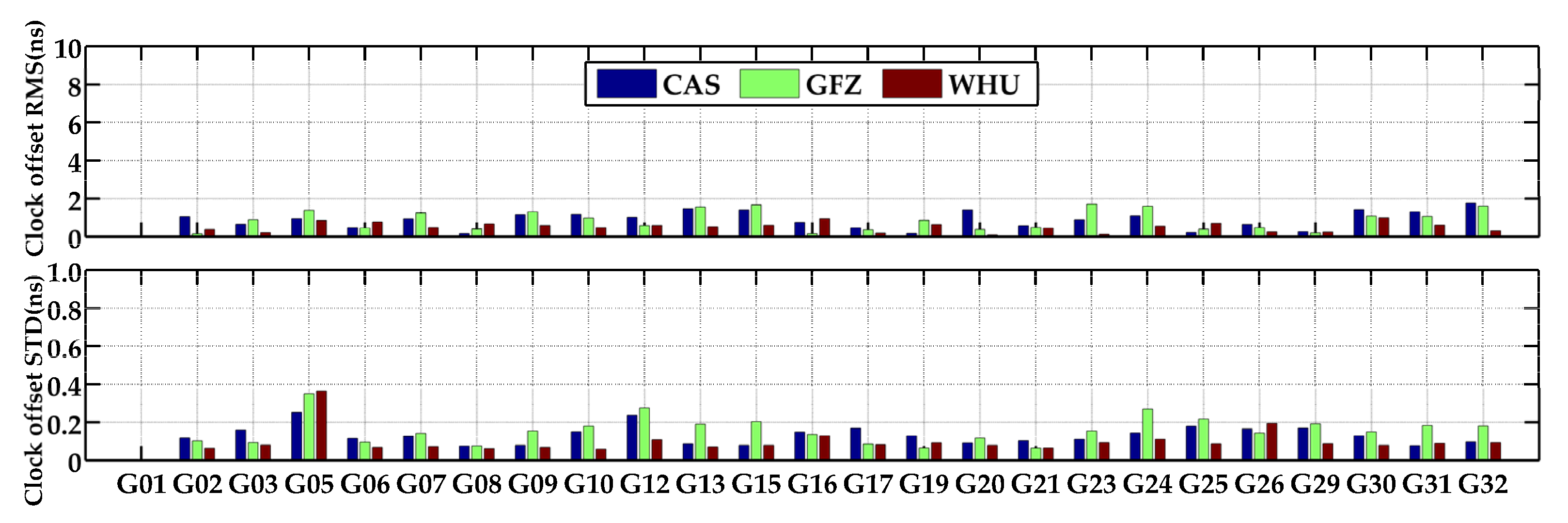
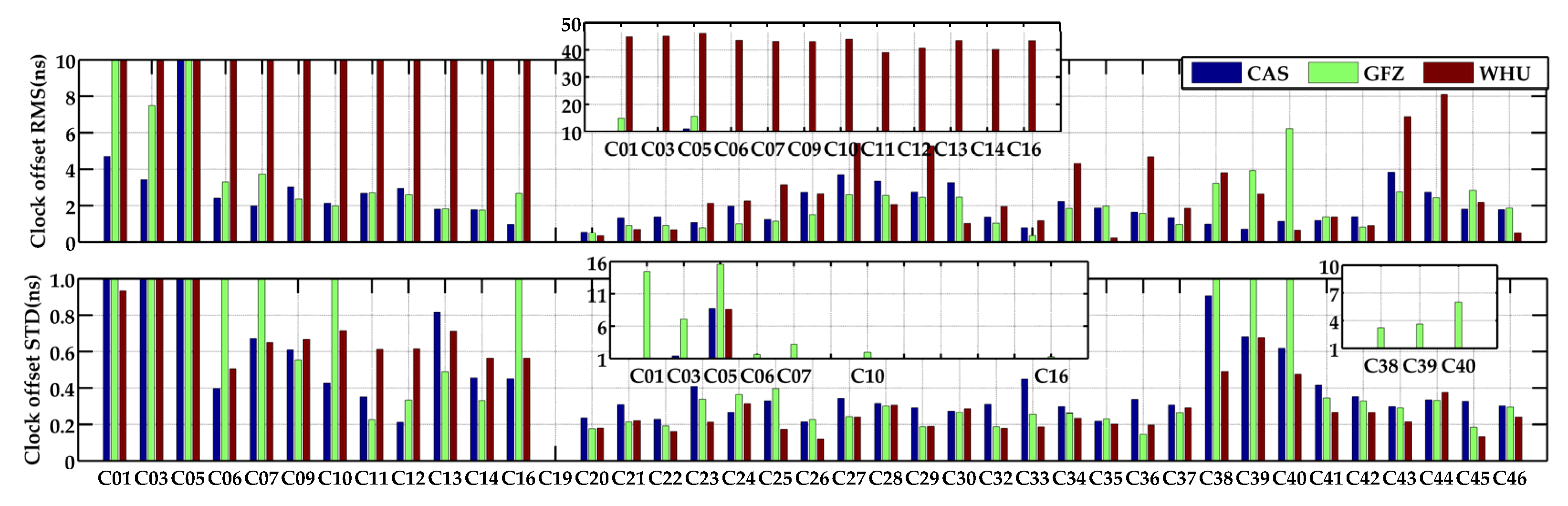
| Analysis Center | GPS (ns) | BDS (GEO + IGSO + MEO) (ns) | BDS (MEO) (ns) | |||
|---|---|---|---|---|---|---|
| RMS | STD | RMS | STD | RMS | STD | |
| CAS | 0.85 | 0.13 | 2.22 | 0.64 | 1.94 | 0.30 |
| GFZ | 0.84 | 0.15 | 2.83 | 1.69 | 1.61 | 0.26 |
| WHU | 0.49 | 0.10 | 14.94 | 0.59 | 6.65 | 0.26 |
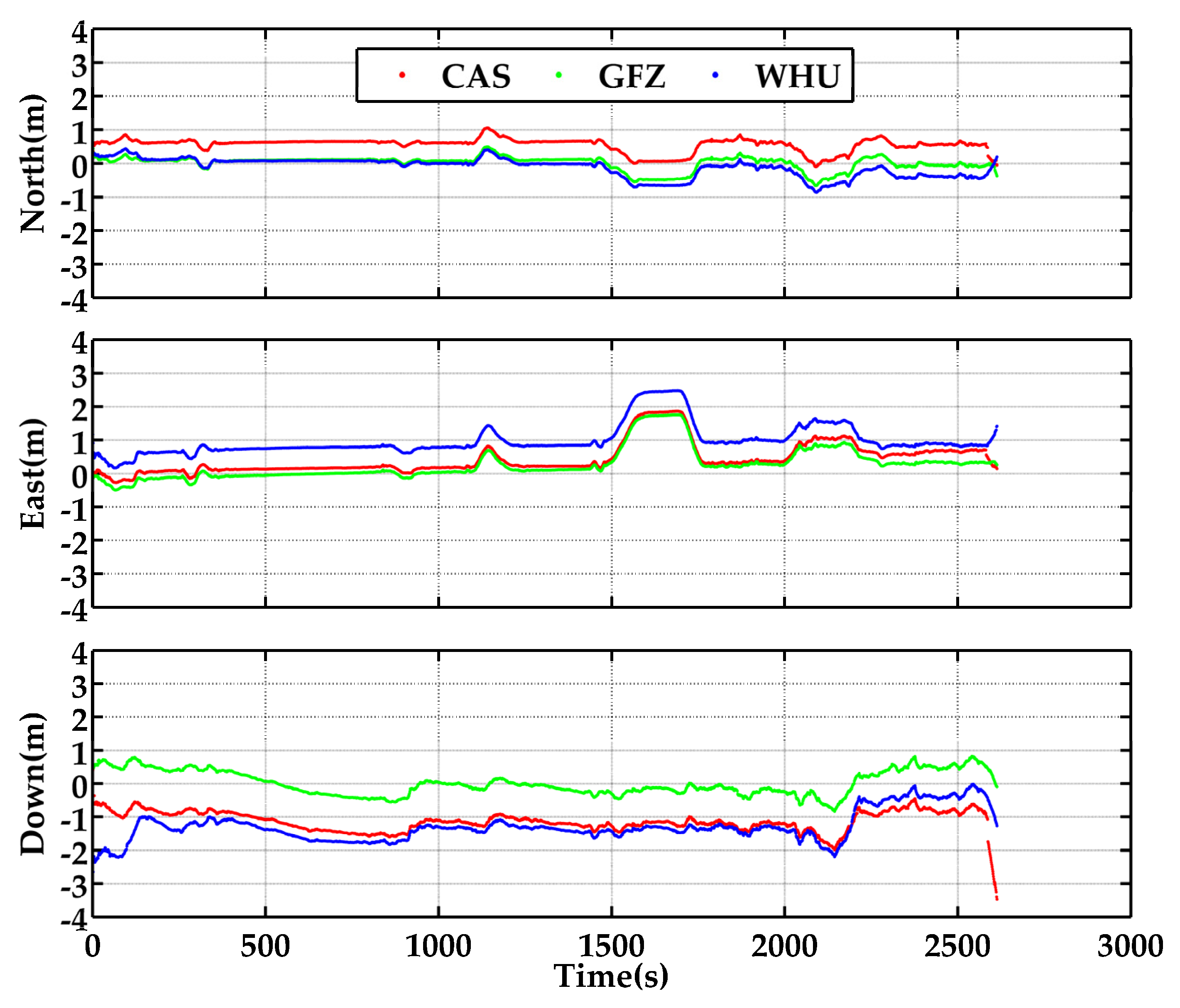
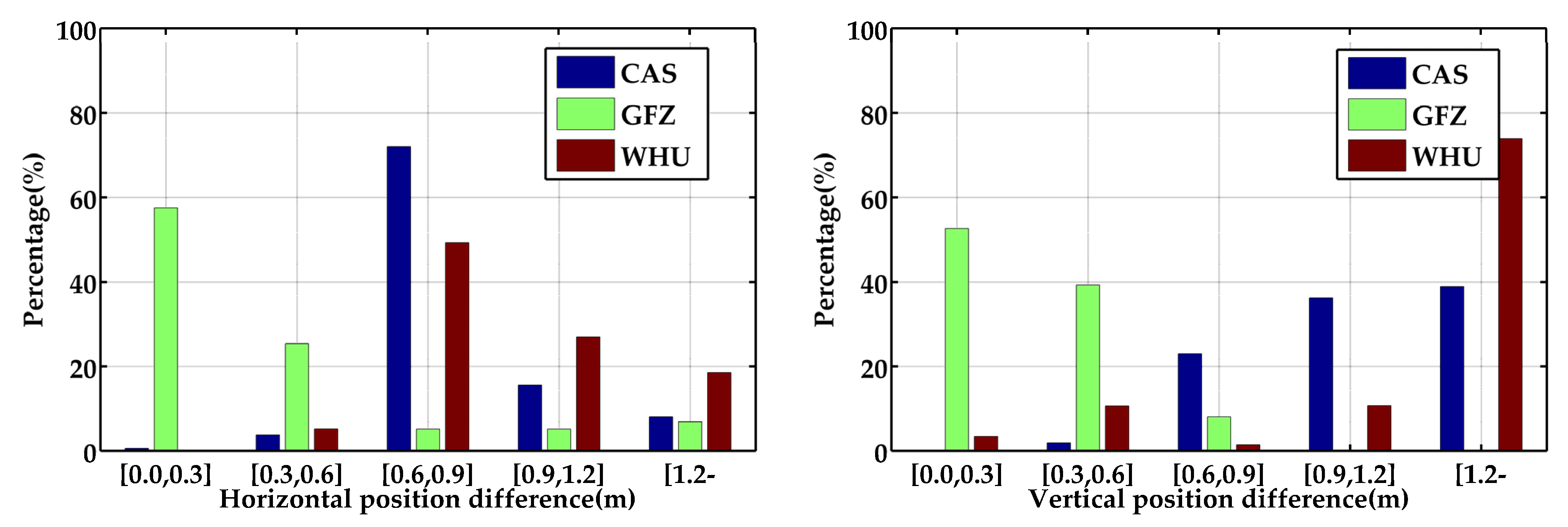
| Analysis Center | RMS (m) | STD (m) | ||||
|---|---|---|---|---|---|---|
| North | East | Down | North | East | Down | |
| CAS | 0.597 | 0.637 | 1.177 | 0.209 | 0.463 | 0.319 |
| GFZ | 0.206 | 0.542 | 0.368 | 0.205 | 0.471 | 0.367 |
| WHU | 0.296 | 1.086 | 1.369 | 0.275 | 0.460 | 0.458 |
| Analysis Center | Attitude (°) | Velocity (m/s) | ||||
|---|---|---|---|---|---|---|
| Roll | Pitch | Heading | North | East | Down | |
| CAS | 0.032 | 0.032 | 0.975 | 0.033 | 0.033 | 0.010 |
| GFZ | 0.027 | 0.027 | 0.489 | 0.033 | 0.033 | 0.008 |
| WHU | 0.020 | 0.019 | 0.523 | 0.033 | 0.032 | 0.007 |
Publisher’s Note: MDPI stays neutral with regard to jurisdictional claims in published maps and institutional affiliations. |
© 2022 by the authors. Licensee MDPI, Basel, Switzerland. This article is an open access article distributed under the terms and conditions of the Creative Commons Attribution (CC BY) license (https://creativecommons.org/licenses/by/4.0/).
Share and Cite
Lv, J.; Gao, Z.; Xu, Q.; Lan, R.; Yang, C.; Peng, J. Assessment of Real-Time GPS/BDS-2/BDS-3 Single-Frequency PPP and INS Tight Integration Using Different RTS Products. Remote Sens. 2022, 14, 4367. https://doi.org/10.3390/rs14174367
Lv J, Gao Z, Xu Q, Lan R, Yang C, Peng J. Assessment of Real-Time GPS/BDS-2/BDS-3 Single-Frequency PPP and INS Tight Integration Using Different RTS Products. Remote Sensing. 2022; 14(17):4367. https://doi.org/10.3390/rs14174367
Chicago/Turabian StyleLv, Jie, Zhouzheng Gao, Qiaozhuang Xu, Ruohua Lan, Cheng Yang, and Junhuan Peng. 2022. "Assessment of Real-Time GPS/BDS-2/BDS-3 Single-Frequency PPP and INS Tight Integration Using Different RTS Products" Remote Sensing 14, no. 17: 4367. https://doi.org/10.3390/rs14174367
APA StyleLv, J., Gao, Z., Xu, Q., Lan, R., Yang, C., & Peng, J. (2022). Assessment of Real-Time GPS/BDS-2/BDS-3 Single-Frequency PPP and INS Tight Integration Using Different RTS Products. Remote Sensing, 14(17), 4367. https://doi.org/10.3390/rs14174367