Article

Passive Acoustic Monitoring as a Tool to Investigate the Spatial Distribution of Invasive Alien Species

by
José W. Ribeiro, Jr.
*,
Kristopher Harmon
,
Gabriel Augusto Leite
,
Tomaz Nascimento de Melo
,
Jack LeBien
and
Marconi Campos-Cerqueira
Rainforest Connection, Science Department, 440 Cobia Drive, Suite 1902, Katy, TX 77494, USA
*
Author to whom correspondence should be addressed.
Remote Sens. 2022, 14(18), 4565; https://doi.org/10.3390/rs14184565
Submission received: 1 July 2022 / Revised: 16 August 2022 / Accepted: 31 August 2022 / Published: 13 September 2022

Abstract

:
Invasive alien species (IAS) are a threat to biodiversity and ecosystem function worldwide. Unfortunately, researchers, agencies, and other management groups face the unresolved challenge of effectively detecting and monitoring IAS at large spatial and temporal scales. To improve the detection of soniferous IAS, we introduced a pipeline for large-scale passive acoustic monitoring (PAM). Our main goal was to illustrate how PAM can be used to rapidly provide baseline information on soniferous IAS. To that aim, we collected acoustic data across Puerto Rico from March to June 2021 and used single-species occupancy models to investigate species distribution of species in the archipelago and to assess the peak of vocal activity. Overall, we detected 16 IAS (10 birds, 3 mammals, and 3 frogs) and 79 native species in an extensive data set with 1,773,287 1-min recordings. Avian activity peaked early in the morning (between 5 a.m. and 7 a.m.), while amphibians peaked between 1 a.m. and 5 a.m. Occupancy probability for IAS in Puerto Rico ranged from 0.002 to 0.67. In general, elevation and forest cover older than 54 years were negatively associated with IAS occupancy, corroborating our expectation that IAS occurrence is related to high levels of human disturbance and present higher occupancy probabilities in places characterized by more intense human activities. The work presented here demonstrates that PAM is a workable solution for monitoring vocally active IAS over a large area and provides a reproducible workflow that can be extended to allow for continued monitoring over longer timeframes.

1. Introduction

Invasive alien species (IAS) are one of the largest threats to biodiversity around the world [1]. It is estimated that the global costs of damage caused by IAS exceed hundreds of billions of U.S. dollars a year [2,3] and that IAS have negatively affected more than a hundred critically endangered native terrestrial vertebrates [4]. The number of established IAS has exponentially increased during the last century for different biological groups [5], and climate change is expected to further expand the distribution of some invasive species [6]. After reaching and becoming established in a new area, IAS can impact local biodiversity through direct and indirect negative interactions with native taxa, such as predation, competition, disease spread, predator poisoning, and altering habitat characteristics [2]. The impact of introducing an alien species can be even more dramatic for native species on islands, which may experience rapid extirpation of native fauna after the arrival and establishment of an IAS [7,8,9]. Insular species often have small populations and home ranges, low genetic diversity, and lack morphological adaptations against IAS [7]. Islands in warmer regions of the globe are hotspots for IAS and tend to have more established invasive species than mainland areas, generating a profound concern for the conservation of native species on tropical islands [5,8].
One of the main obstacles that wildlife managers and conservationists face in opposing the threat of invasive species is acquiring rapid, reliable, large-scale baseline information on the distribution of fauna—data which are critical in guiding effective wildlife management programs [10]. A central challenge to this type of monitoring is how to cover a large sampling area with a limited number of researchers (an issue faced by many projects and agencies) and still complete surveys in a short period of time, which has the dual benefit of avoiding temporal bias and providing distribution data quickly. Moreover, the success of IAS control or eradication efforts is typically greater when species are detected in an early stage before they become established in a new location [11]. Therefore, the development of early-stage detection systems is urgent in order to identify IAS before they can become a significant threat [12,13,14]. The rapid evolution of remote sensing tools has made it possible to conduct large-scale monitoring in a short period of time, providing detailed baseline information of ecosystems and biodiversity [15].
Remote sensing through satellite and airborne images has been successfully used to detect and monitor changes in forest cover, vegetation type, disturbance regimes, plant phenology, and ecosystems [16,17,18,19,20]. However, remote sensing is still mostly overlooked for invasive fauna, though camera traps and autonomous acoustic devices have been successfully used to detect and monitor alien animal species [15,21,22]. Other noninvasive methods such as eDNA have also been used recently to detect IAS [21,22]. The emergence of new autonomous recording units (ARUs) and platforms to store and analyze massive amounts of audio data has greatly improved the utility of passive acoustic monitoring (PAM) to monitor soniferous wildlife and its threats [23,24,25,26,27,28]. Taxa that regularly produce species-specific vocalizations, such as birds, anurans, bats, insects, and some mammals, are well suited for ecoacoustic surveys [29,30]. Although PAM has great potential for monitoring biodiversity and researching a variety of ecological issues [31], it has not been used yet to its maximum potential for investigation of soniferous terrestrial IAS [32,33]. However, PAM has been used for investigating the occurrence of invasive freshwater drum in the New York State Canal System and assessing the phenology of the invasive cane toad in Australia [34,35].
Passive acoustic monitoring has numerous benefits for rapid assessment and early detection of sound-producing fauna, as well as large-scale and long-term monitoring, and can decrease the response time for managing soniferous IAS [28,31,33,36]. Amongst the primary benefits, PAM is a standardized noninvasive survey method that can be used simultaneously in numerous locations, allowing for the monitoring of hundreds to thousands of sites at the same time, which would otherwise be impossible if trained researchers were required to be in the field at each location [36]. Additionally, PAM facilitates sampling during all periods of the day, covering the peak of activity of different taxa; devices can be easily deployed with little or no specialized training; and recordings can be permanently stored, providing insights on temporal patterns of biodiversity [36,37].
Passive acoustic monitoring generates the detection and non-detection data required for species distribution models, one of the most used tools for IAS risk assessment [38,39,40,41,42]. Due to the substantial volume of data collected by the ARU in the field, one constraint on PAM has been the ability to examine all of the recordings collected. As a result, the development of protocols that optimize inspection of recordings together with semiautomatic or automatic techniques that speed up data analysis is necessary to extract the maximum amount of information from the acoustic data collected. In addition, to expedite biological and ecological insights from data acquired through PAM, it is important to develop user interface tools that allow availability, visibility, and management of results for the nonacademic public (e.g., citizen scientists, birdwatchers, practitioners, and wildlife managers).
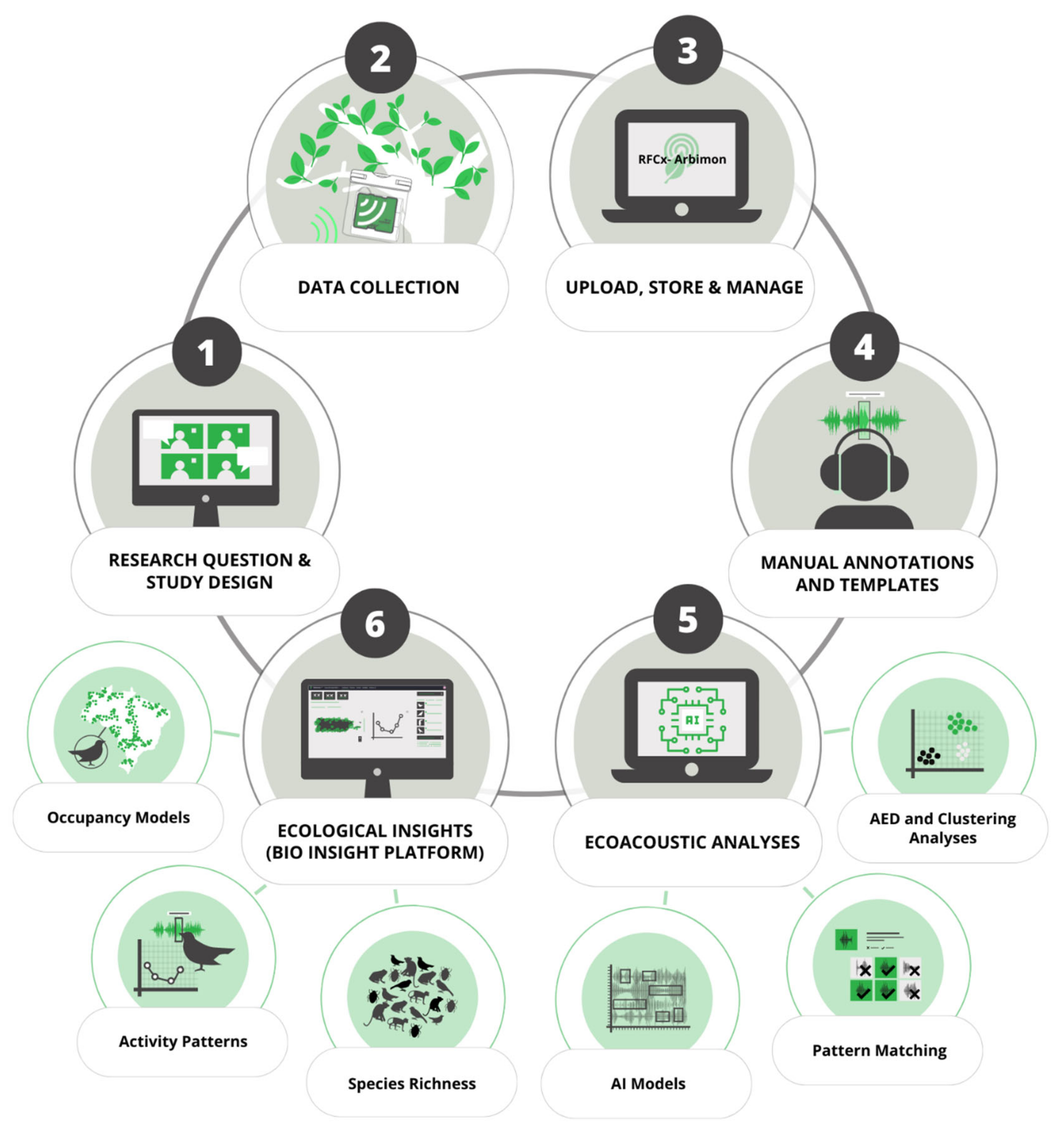
Here, we used a large-scale PAM survey across the Puerto Rican archipelago (841 sampling sites) to investigate the spatial distribution and peak of vocal activity of IAS. Our main goal was to generate baseline population data for soniferous native and IAS in Puerto Rico. Moreover, we provide a roadmap on how remote soundscape data collection can be used to rapidly provide distribution information for soniferous species through a free, user-friendly web interface designed to be accessible to diverse stakeholder groups as biologists, ecologists, wildlife managers, and citizen scientists. Our workflow offers a balance between manual inspection of recordings with semiautomatic analysis, which considerably reduces the time required to analyze the large amount of data typically generated by PAM, and providing assessment for the peak activity of species and detection/nondetection data for each day and site sampled. To assess the status of IAS populations in Puerto Rico, we used Bayesian single-species occupancy models to investigate how the spatial distribution of IAS varied through environmental gradients. The last step of our end-to-end pipeline for large-scale passive acoustic monitoring consisted in the development of a web page connecting and summarizing data from the Arbimon platform to display and share the results of the ecoacoustic analyses and close the gaps between academia and wildlife managers and decision makers. We expect that our study can provide baseline information on soniferous IAS for wildlife managers and decision makers in Puerto Rico and support future research focused on the rapid assessment or long-term monitoring of sound-producing wildlife across a broad spatial area using acoustic survey methods.

2. Materials and Methods

2.1. Passive Acoustic Monitoring

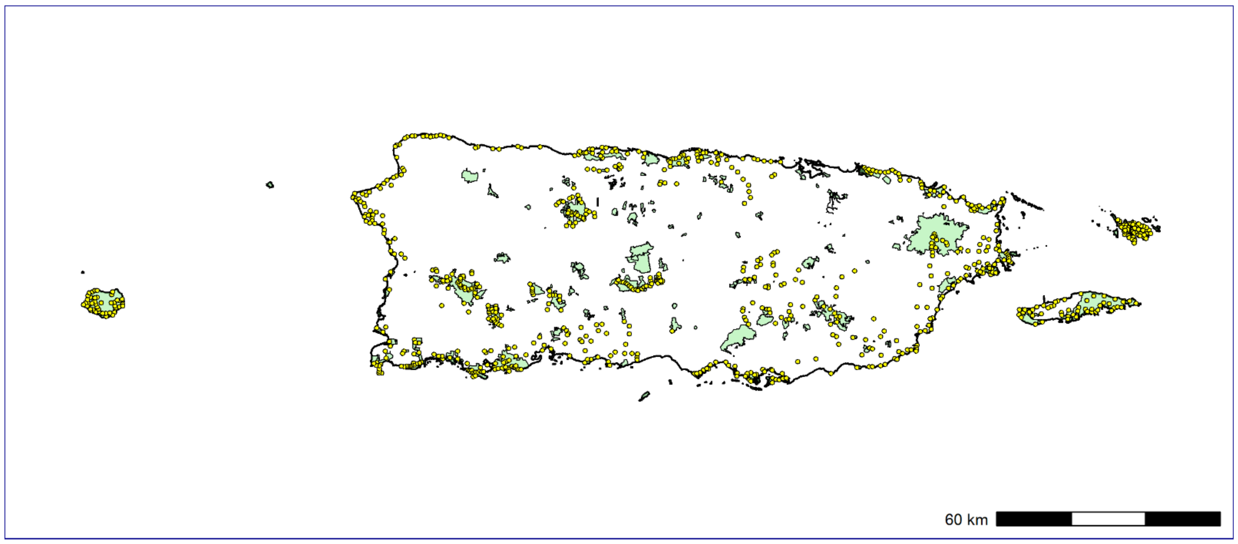
The Caribbean is a hotspot of biodiversity [43]; unfortunately, the islands in the region are also hotspots of established IAS [8]. Amongst them, Puerto Rico has a long history of IAS, which raises concerns about the prior and future impacts of those species on the native and endemic flora and fauna [44,45]. There is a gap in the knowledge of population assessment of IAS in the archipelago, primarily for birds and frogs. We conducted a large-scale PAM survey in the Puerto Rican archipelago, including the main island of Puerto Rico and the major offshore islands of Culebra, Desecheo, Mona, and Vieques (Appendix A). Overall, we successfully deployed ARUs at 841 sites: 198 sites in and around six preselected regions in the interior of Puerto Rico and 643 sites distributed in 14 regions across coastal areas in the main island of Puerto Rico (n = 485 ARU), Culebra (n = 49), Desecheo (n = 7), Mona (n = 52), and Vieques (n = 50). The selection of sampling sites within each region and protected area followed an approximate systematic sampling design to capture the full range of conditions found there.
We made use of lightweight and low-cost Open Acoustic Devices AudioMoth recorders to record the soundscapes across Puerto Rico [26,36]. We used the Open Acoustic Devices AudioMoth Configuration App to program the audio devices to record 1 min every 5 min with mean gain and at a 48 kHz sampling rate. Four teams of two field agents deployed AudioMoths between 1 March and 6 June 2021. The ARUs were placed in a protective waterproof plastic case and then affixed to a tree/vine/shrub using wooden clothespins at a height of 1.5 m (Appendix A). A total of approximately 200 AudioMoths were simultaneously in the field at any given time during the survey period; the AudioMoths were rotated across sampling sites after about 1 week of data collection, with ARUs simultaneously in the north, south, east, and west of the island at all times. The AudioMoths recorded in the field for at least seven consecutive days; thereafter, field agents revisited each site to retrieve the ARUs that had been deployed and move them to a new location. Due to logistical issues and the occasional malfunction of the devices, the number of days recorded at a site ranged from 1 to 11 (mean = 8.3, sd = 1.11). The main factors contributing to data loss or site failure were device malfunction (n = 10) and theft (n = 4).
We made an effort to deploy the ARUs no less than 200 m apart from each other, which was an adequate distance to ensure that a calling event of most species was not recorded by more than one device simultaneously (the great majority of the distances between nearest points were above 500 m; mean = 865.03 m, sd = 714.05). Moreover, we expected that 200 m was a good proxy of the home range of most low-vagility forest birds and frogs, ensuring site independence for these species. Field agents manually documented the date, site ID, recorder ID, latitude, longitude, and additional relevant climate and environmental factors. The Rainforest Connection (RFCx) Companion App was also used during AudioMoth deployments to sync the ARUs and add site metadata (e.g., GPS coordinates, elevation, photos, and notes) with sites in the RFCx Arbimon web platform (https://apps.apple.com/us/app/rainforest-connection/id1178078181 (accessed on 1 March 2021)). Once the ARUs were retrieved, all recordings were uploaded to RFCx Arbimon web-based platform, where all the sound files are now permanently stored (https://arbimon.rfcx.org/project/puerto-rico-island-wide/dashboard (accessed on 5 July 2021)).

2.2. Semiautomatic Species Identification Workflow

Large-scale and long-term investigations using ARUs commonly generate a colossal number of recordings [27], quantities that quickly become unworkable to examine through manual approaches. We developed a protocol for acquiring species detections from audio recordings using a semiautomated procedure that requires a relatively small time investment from researchers to produce a preliminary list of species occurring in a study area and provides a validation data set [46,47,48,49] (Figure 1). RFCx Arbimon is a free, cloud-based, user-friendly acoustic analysis platform for storage, management, visualization, and analysis of ecoacoustic data. Using the spectrograms generated by Arbimon, two of the coauthors with extensive experience in audio surveys (G.A.L. and T.N.M.) manually inspected all 1-min recordings from two nonconsecutive days at each site (576 1-min recordings per site were inspected) to search for species’ sound signals and noted if each species call was present in each record [49]. During this process, hereafter referred to as “manual annotation”, animal sounds with a high signal-to-noise ratio were identified and selected as the templates for template-matching analyses, known as Pattern Matching (PM) analysis in the RFCx Arbimon system [49] (Figure 1). During these steps we identified and tagged other characteristics and sound sources such as the quality of recordings, noises caused by internal malfunction of AudioMoth devices, external interference, anthrophony (e.g., noise of machines, vehicles, and voices), and domestic animals. This manual annotation of the data was an important step in providing a consistent preliminary list of species recorded by ARUs throughout the study area, selecting good templates for PM analysis, and generating validated data sets [23,46,49].
The preliminary species list created by the manual annotation of a subset of recordings provided the templates that were subsequently used to select species of greatest conservation need (SGCN; https://www1.usgs.gov/csas/swap (accessed on 30 September 2021)), native and endemic species and all IAS detected for the ecological analyses. We ran a PM analysis for a total of 65 species in the RFCx Arbimon platform (37 SGCN, 16 IAS and 12 extra species). Using available audio libraries (e.g., Xeno-Canto) we also created PMs for other SGCN and IAS that are known to occur in Puerto Rico but were not detected during the manual validation or that did not have acceptable templates. Use of external templates did not result in the detection of any new species. Pattern Matching, a template-based detection algorithm, take a sound template and an audio file playlist as inputs and searches a selected playlist for signals that correlated with the template in the spectrogram domain [46]. All audio segments with a correlation equal to or greater than a user-chosen threshold were detected as regions of interest (ROI) and displayed in a graphical user interface (GUI) in a grid format. We assigned a correlation threshold equal to 0.2 and ran the models on all sites included in the playlists. The selection of a low threshold resulted in a high number of false positives, though the number of false negatives was assumed to be negligible. M.C.C., G.L. and T.M. manually reviewed the template-matching results. In this step, we annotated the results as either positive or negative to indicate the corresponding species’ presence or absence, respectively. This ensured that the final data set used in the analyses only included expert-verified detections and excluded all false-positive detections.
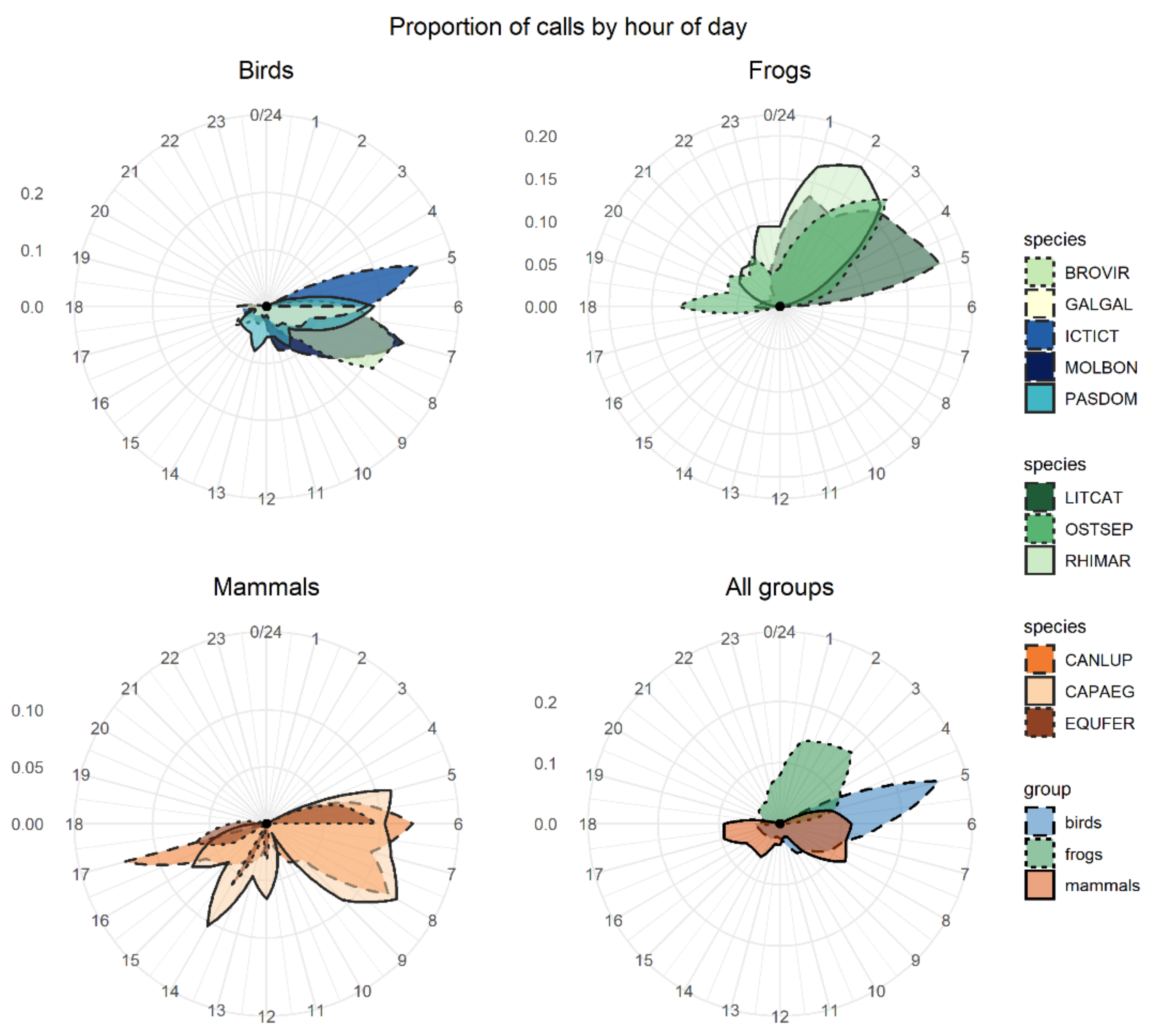
We created two playlists on which to run the PM: a diurnal playlist with all recordings from 5 a.m. to 6 p.m. and a nocturnal playlist with all recordings from 6 p.m. to 5 a.m. The diurnal playlist was applied to 41 bird species and three mammal species; the nocturnal playlist was applied to 18 frog species and three bird species. The resulting ROIs from the PM analysis were manually inspected in a grid view and validated as true or false positives by experts. For validation, we filtered the results to only show the best-scored ROI per site and day to acquire detection and nondetection data to be used in the occupancy models (Figure 1). The PM analysis of all species detected using all recordings together with the manual validation of the best-scored ROI per site and day took two ornithologists (GAL and TNM) approximately 15 days. Using these validations, we created a table of sampling sites by sampling days for each species (i.e., 1 if the species was detected, otherwise 0). Since our main objective here was not to investigate the daily activity of these species but to maximize detection in each sampling site, we chose the period with the greatest volume of soniferous data for the birds and frogs based on our experience working with the birds and frogs of Puerto Rico. Thus, we highlight that the polar plots for birds and mammals were biased for the diurnal period while those for frogs and nocturnal birds were biased for the nocturnal period. However, if the research goals involve investigating the daily activities of species, this approach can be easily adjusted to incorporate both periods of day for each species.
In this paper, we used the standard biological sense adopted by Simberloff (2013) [2] that defines invasive species as “species that arrive with human assistance, establish populations, and spread”, contrary to the usage adopted by policymakers who assume that IAS are only introduced species that cause some proven negative impact on diversity or an ecosystem, although there is evidence suggesting that most of these IAS may be threats to Puerto Rico’s biodiversity.

2.3. Explanatory Variables

We collected environmental data from multiple online repositories administered by the Multi-Resolution Land Characteristics Consortium, National Oceanic and Atmospheric Administration, Open Street Map, USDA Caribbean Climate Hub, and USGS EarthExplorer. Data gathered included GIS layers of elevation, climate, forest age, land-use type, protected area extent, and roads and trails. For each sampling location, a buffer was added with a radius of 200 m around the site (area = 12.57 ha). Data for inclusion as environmental covariates in the ecological analyses were extracted for the 200 m site buffers using the Zonal Statistics and Tabulate Area tools in ESRI ArcMap (version 10.8; Environmental Systems Research Institute, Inc., Redlands, CA, USA).
We selected 13 explanatory variables that have been reported to have an effect on fauna from the GIS layers a priori [38,48,51,52]. We checked multicollinearity among the explanatory variables used in the occupancy models through the variance inflation factor (VIF) function of the “usdm” package [53] in R version 3.6 [54]. This function progressively excludes collinear covariates through a stepwise procedure. VIFs were calculated using two methods: VIFcor (threshold = 0.7) and VIFstep (Threshold = 10). The following variables with low collinearity were used in occupancy models: elevation, mean annual precipitation, percent of forested area between 34–54 years old, percent of forested area older than 54 years, percent of area within a protected area boundary, percent of canopy cover, distance from roads, and proportion of built-up area (Appendix B).
We used the Generate Tessellation tool in ArcMap to create a hexagon grid covering the entire extension of Puerto Rico and major offshore islands. The hexagon grid had a cell area equal to that of the 200 m buffer applied to survey sites. We exported values for the explanatory covariates for each hexagon, which were used to make maps of predicted occupancy for each species using the top-ranked model.

2.4. Single-Species Occupancy Model

Since the IAS may have experienced different introduction histories on the islands and have different capabilities to colonize new islands, we chose to model species occupancy only for the islands where the species was detected in at least five sampling sites. We investigated occupancy while accounting for imperfect detection of invasive species by fitting a hierarchical single-season occupancy model [55,56,57] in a Bayesian framework using the “ubms” package in R [58,59]. The occupancy model made use of repeated observations in the sites to disentangle the observational component (i.e., detection/nondetection) from the state variable of interest (i.e., “true” occupancy [38,55]). The model had four central assumptions: (i) independence between sampling sites, (ii) independence between repeated observation occasions, (iii) absence of misidentification of the focal species (no false positive error), and (iv) no colonizations or extinctions during the study period; that is, the sampling sites were expected to be “closed” to the occupancy state of species during the study period [55,60,61]. Assumption of a closed occupancy state may be relaxed if the changes in the occupancy state are random, and therefore the occupancy parameter should be interpreted as the probability that the species “uses” the habitat [62].
We applied a sequential approach to identify the most parsimonious model for each species rather than run all possible model combinations [63]. Firstly, we held the occupancy probability constant (ψ(.)) and fit four a priori candidate models for detection probability: null model, elevation only, linear and quadratic effect of Julian day, and full model (Table 1). Then, we held the top-ranked detection model ( ρ (TM)) and modeled a set of a priori candidate models for the occupancy probability of species (Table 1). Since the availability of the spatial data containing the predictor variables varied across islands, the number of candidate models for the species also varied depending on the island on which the species was detected (Table 1). The parameters of both detection and occupancy were modeled as a logit function [55,59]. We normalized all continuous explanatory variables to have a mean of 0 and a standard deviation of 1 [61].
Even while expecting that 200 m was a sufficient distance to guarantee sampling-site independence, we made the decision to run a spatial occupancy model to account for spatial autocorrelation in the occupancy probability, since including spatial autocorrelation in occupancy modeling can improve species prediction and distribution maps [56,59,64]. We modeled the spatial occupancy model using restricted spatial regression (RSR) that dealt with the random effect uncorrelated with the fixed covariates [64]. We considered that two sites were neighbors if the distance between them was equal to or below 1000 m (we set the threshold at 1000). RSR has been shown to be a good choice for modeling occurrences while accounting for imperfect detection and spatial autocorrelation [59,64]. Due to the long time required to run models with spatial autocorrelation, we chose only to fit RSR with the top-ranked nonspatial occupancy model to determine if incorporating spatial autocorrelation improved the model fit.
We compared the models using Bayesian leave-one-out cross-validation (LOO) [59,65]. The log pointwise predictive density (elpd) was calculated for each model using the modSel function of the “ubms” package [59]; we ranked elpd from highest to lowest since the model with the largest elpd value corresponded to the model with the best accuracy [65]. Additionally, we presented the difference between the elpd of models and the elpd of the top-ranked model (Δelpd) along with standard error of elpd (se of Δelpd). We checked the chains’ convergence of all parameters of the top-ranked model by assessing the effective sample size (n_eff) and R-hat statistic and by visually inspecting traceplots [59]. Furthermore, we assessed the model fit through residual plots for the state and observation variables.
Based on previous studies, we assumed that the IAS would benefit from high levels of human disturbance and present higher occupancy probabilities in places characterized by more intense human activities [45,66]. Therefore, we expected that invasive species occupancy would be negatively related to elevation because human activities are more common and intense in low-elevation areas (e.g., human settlement and agriculture) in Puerto Rico. A higher proportion of protected areas and canopy cover would be inhibitors of invasive species occurrence by representing more preserved environments [66,67,68]. Since the anuran IAS considered in our study do not present striking adaptations to grow and reproduce in conditions with a low availability of water, we predicted a positive relationship between these species’ occupancies and the mean annual precipitation. Additionally, we expect that a proximity to roads and a high proportion of built-up area in a location would positively influence the occupancy of IAS [66].

3. Results

We based our findings on 1,773,287 1-min recordings from 8.9 TB of soundscape data. Our manual inspection of recordings together with PM analysis generated an overall list of 95 species detected throughout the Puerto Rican archipelago: 74 birds, 18 frogs, and 3 mammals (Appendix C). We found 92 species on the main island of Puerto Rico, followed by Vieques, Culebra, and Mona with 31, 25, and 19 species, respectively (Appendix C). Overall, 16 species were considered invasive species (Appendix C) and are potential threats to wildlife in the Puerto Rico: 10 birds (Icterus, Molothrus bonariensis, Gallus gallus domesticus, Brotogeris versicolurus, Passer domesticus, Amazona amazonica, Amazona viridigenalis, Bubulcus ibis, Myiopsitta monachus, and Streptopelia decaocto), 3 frogs (Lithobates catesbeianus, Osteopilus septentrionalis, and Rhinella marina), and 3 mammals (Canis lupus familiaris, Capra hircus, and Equus ferus caballus).
None of the invasive species were detected on Desecheo Island; therefore, this island was not used in the occupancy model. The wild goat (C. hircus) was detected at 21 sites, all of which were on Mona Island. Feral horse (E. ferus caballus) was detected at 11 sites on Vieques and two sites on the mainland; therefore, the occupancy model was performed only for Vieques. Chickens (G. gallus domesticus), Venezuelan troupial (I. icterus), shiny cowbird (M. bonariensis), and domestic dog (C. lupus familiaris) were the most widespread species, detected at 165, 131, 78, and 76 sites, respectively. Chickens (the only IAS for which the occupancy model was fitted for more than one island) were detected at 134 sites on the main island, 27 sites on Culebra, 3 sites on Vieques, and 1 site on Mona. Five bird species (A. amazonica, A. viridigenalis, B. ibis, M. monachus, and S. decaocto) had low raw detections and were detected at few sites (less than 10 sites); thus, we did not run occupancy models or a call activity pattern analysis for them. The other IAS detected were found at between 12 and 24 sites (American bullfrog (L. catesbeianus), house sparrow (P. domesticus), Cuban tree frog (O. septentrionalis), cane toad (R. marina), and white-winged parakeet (B. versicolurus)).
The number of calls recorded and the peak of activity varied greatly between species (Figure 2). The group with the highest number of detections (i.e., best-scored ROI per site and day) was birds (e.g., chicken had more than 750 raw detections, Venezuelan troupial had 450 detections, and shiny cowbird had 194 detections), followed by mammals (ranging from 23 to 148 detections) and frogs (ranging from 53 to 75 detections). The bird species had a high activity peak early in the morning (between 5 a.m. and 7 a.m.). The peak activity of frog species varied between 1 a.m. and 5 a.m. depending on the species. The American bullfrog had a peak in calling activity at dawn (about 6 a.m.); the cane toad showed a peak at 2 a.m.; and the Cuban tree frog showed two peaks of activity, with the strongest at 3 a.m. and a second less-intense peak at dusk. Mammals did not show a clear calling activity peak.
We fit occupancy models for 11 IAS (all 3 frog and mammal IAS and 5 species of birds). In general, the occupancy models presented good convergence and fit well for the species when checked through the inspection of traceplots (Appendix D) and using R-hat statistic values <1.1 (Appendix E). However, the “top-ranked” spatial occupancy model of the Cuban tree frog did not show good convergence and efficiency diagnostics for Markov chains (ψ(fa2 + fa3 + RSR-1000); ρ (elevation + date + date2)) even after running the model with 200,000 interactions; thus, we used the second-best model for the species to show the parameter estimates (Table 2; Appendix E). In general, the probability of detecting IAS throughout Puerto Rico was medium to low and varied widely, ranging from 0.002 to 0.63 (Appendix E); most species were below 0.3. The best model that explained the detection probability of all species (except for feral horse, white-winged parakeet, and the two domesticated species) included the three predictor variables: elevation, Julian date linear, and Julian date quadratic (Appendix E). In general, the Julian date positively influenced a species’ mean detection probability. The relationship between elevation and the detection probability varied depending on the species.
Occupancy probability ranged from 0.002 (American bullfrog) to 0.67 (wild goat on Mona). The three amphibian IAS showed a very low occupancy probability (lower than 0.08). The results showed that elevation and precipitation were the variables that best explained the occupancy probability of IAS in Puerto Rico and appeared in the top-model of six species, followed by proportion of forest cover aged between 32–54 years (fa2) and forest cover older than 54 years (fa3; Table 2). The best model selected for four of the species (shiny cowbird, cane toad, wild goat, and house sparrow) was the null model containing only the intercept.
We created maps of model-predicted species occupancy probability across Puerto Rico and outlying islands for the 11 invasive species with occupancy models (Figure 3; Appendix F). Here, we exemplify the predicted occupancy of the Venezuelan troupial (see Appendix F for the occupancy prediction maps for the other species). We chose the Venezuelan troupial as an example because it was the species that showed the top-ranked model with the highest difference between the other a priori candidate models, which suggested more confidence in the top-ranked model (higher ΔELPD between the top-ranked and second-best models). We limited the forecast map to the islands where the occupancy model was fitted for each species to diminish spurious predictions because the gradients between islands were different. The point-estimates occupancy probability map for the Venezuelan troupial in Puerto Rico in 2021 under the top-ranked occupancy model suggested a high probability of the species occurring in regions close to the coast, mainly in the south and southwest of the main island (Figure 3).
We developed a website (https://bio.rfcx.org/puerto-rico-island-wide (accessed on 14 June 2022)) with the purpose of data sharing and summarizing the results of the study for the use of government agencies (e.g., Departamento de Recursos Naturales y Ambientales (DRNA), U.S. Fish and Wildlife Service) and the general public (e.g., educators and birdwatchers). The website contains information on the vocalizations, distribution, and ecology of the species detected at the 841 sampling sites in Puerto Rico during the project, including a searchable database with detection data, presence/absence maps, and occupancy maps for all birds, mammals, and anurans recorded (Appendix G). All maps, plots, and data used to generate the figures can be freely downloaded. The data and figures on the website are continuously updated according to new acoustic data as they become available.

4. Discussion

The acquisition of population baseline data for native and invasive species is a fundamental step in monitoring and managing wildlife in dynamic land cover and climate change scenarios. However, detecting and monitoring animal species at large spatiotemporal scales, especially in the tropics, remains a significant challenge. In this study, we presented an end-to-end acoustic monitoring pipeline that was able to detect several soniferous native, endemic, threatened, and invasive species; access their current population status; and summarize and display results in a user-friendly platform.
Converging with our expectations, the occupancy probabilities of IAS were generally lower in environments with less human disturbance. For example, the occupancy probabilities of some IAS were negatively associated with elevation (five species) and forest older than 54 years (four species). These findings suggested that IAS may be favored by human activities because species occupancies were higher in new forest areas that were expected to be more disturbed and human activities are more common and intense at low elevations in Puerto Rico. Our findings were in agreement with an overall correlation between anthropogenically disturbed habitats and invasive species of plants, invertebrates, fishes, birds, frogs, and mammals [45,66,67,69]. Our results revealed that elevation and precipitation were the most important variables for explaining the distribution of most soniferous IAS (the best model for 6 of 11 IAS contained elevation and precipitation as explanatory variables), followed by proportion of forest cover aged between 32–54 years (fa2) and forest cover older than 54 years (fa3).
Free-range pets and domesticated species can also have a negative impact on native species, especially in island ecosystems [68,70]. Although the chicken, dog, wild goat, and feral horse are domesticated species, we decided to include them in the acoustic analysis because they can impact native wildlife directly (e.g., predation) and indirectly (e.g., spreading diseases and impacting on vegetation) [71]; moreover, some feral populations exist in the archipelago. Some studies have shown that domesticated species (such as dogs) can occur widely within protected areas and may represent a threat to native species [72,73]. In contrast, our occupancy models suggested a lower probability of dogs and chickens occupying the protected areas on the main island of Puerto Rico (Appendix E and Appendix F), indicating that protected areas can offer some level of protection against domesticated species.
Our knowledge about the main drivers of IAS distribution is still limited, which was reflected in the model-selection process. The null model was the top-ranked model of four species, indicating that the explanatory variables utilized in the models were not good predictors of spatial variation of these species. The anuran IAS showed a low probability of occupancy (<0.07) in the landscape of the main island of Puerto Rico, which may have reflected the low natural availability of aquatic environments in the landscape (i.e., natural low occupancy probability of species) or may have been a result of our sampling design, which was not focused on lentic systems. The three frog IAS had call activity associated with ponds; a new sampling process could easily be designed to include more lentic systems, which would increase the chance of finding frogs with an aquatic life stage.
Estimating the probability of detection and occupancy of IAS can facilitate more efficient management actions because the estimations of parameters related to species occurrence on the landscape will be unbiased and provide an uncertainty measure [74,75]. In our study, most IAS showed a higher probability of detection at the end of the sampling period (late May and early June 2021), suggesting that most species were more vocal and thus more easily detected by PAM at the end of the early high rainfall season. These findings were congruent with breeding activity peaks recorded for terrestrial birds in Puerto Rico [52]. This positive relationship was restricted to the temporal range of the study (March–June) because a year-round sampling design can have more variability and alter the relationship between the Julian day and detection probability.
Despite the large volume of data analyzed through PM, five birds were detected at only a few sites (<10), and we did not run occupancy models for them due to the small number of detections (see Appendix H for detection locations). This low detection rate could correspond to a “real” low occurrence/density of the species in the study area or might have resulted from the species vocalizing sparingly. Even with a low number of detections, knowing where these species were found can present a valuable opportunity to prioritize surveying of locations closely similar in geographical and environmental space where the species were detected. Although working with few detection points (or even one detection point) is challenging and has several limitations, it can be useful in directing resources and field survey efforts to find undetected populations of a “rare” species in a region [76] and monitor possible early-stage expansions.
The detection/nondetection of species is a baseline outcome of audio data analysis that can be used in various ecological analyses that make use of this type of data [28,36,38]. For example, the diel and annual activities of species are fundamental aspects of their life history, and the knowledge of it can be used along with artificial advertisement calls to trap and manage IAS [35,77,78]. We found that diel call activity of the species groups greatly varied, suggesting that monitoring and management programs should focus on specific periods of the day to increase their chance to detect and capture the IAS.
Our end-to-end pipeline provided an effective method for detecting several native, endemic, threatened, and IAS (16 species) in Puerto Rico, including birds, frogs, and mammals (95 species were detected overall). The manual validation of best ROI per site per day of PM analysis detected around 2000 call events of IAS. We took less than two days to validate the PM of the 16 IAS following our workflow. The fast analysis of this vast data set (1,773,287 1-min recordings) was only possible through a user-friendly web-based platform with annotation functionality and the creation of user-defined playlists that allowed us to combine manual annotations with PM analysis and validations by experts (see Figure 1). While users can take advantage of a variety of available software platforms or develop their own code to analyze PAM data, multifunctional tools that have user-friendly interfaces are necessary to speed up and increase usage of PAM by a wider audience with varying skill sets [79]. Free user-friendly interfaces may be an effective way to implement early-stage detection and assist in the long-term monitoring of IAS populations by conservationists, wildlife managers, and decision makers. Cloud-based platforms such as those used in this project also can facilitate the inclusion of citizen scientists and other experts to improve and speed up the validation of data from the target groups.
Detection and monitoring of IAS is of increasing importance for informing conservation management. Tools using an intuitive GUI can improve data exploration and narrow communication and knowledge gaps between the scientific community and other groups [80]. Here, we introduced a webpage as part of the last step of the Arbimon ecosystem, filling a critical need for a practical and intuitive way to summarize, display, and share ecological results from acoustic-monitoring processes so that the data generated can be easily used and shared by and with environmental agencies. This web-based tool was designed to display biodiversity indicators such as number of detected species, activity patterns, and species occupancy over maps and plots that can support species management.
Previous studies have shown the benefit of combining acoustic monitoring with occupancy modeling to understand native species distribution [38,51,81,82,83]; in accordance with these findings, our study reinforced that this approach can be useful to understand the distribution of soniferous IAS as well. Additionally, our approach generated detection/nondetection data from species of greatest conservation need beyond IAS that can be used in more complex models (e.g., two-species or multispecies models) to assess relationships and interactions between IAS and SGCN, which can help researchers to understand the potential effects of IAS on native species detection and occupancy probabilities [84,85,86]. PAM has been shown to be very useful for investigating IAS, and there remain a number of avenues for expansion. Other studies have demonstrated the usefulness of PAM as a consistent tool to examine sounds in nature, involving a range of topics [27] such as monitoring native wildlife species [49,82,87], disturbance from human noise [88,89], agricultural pests [90], ecosystem functions [91], disease-transmitting mosquitoes [92], gunshots [93,94], and illegal timber harvests [95]. Although automated techniques are emerging to deal with the massive amount of acoustic data that are intrinsic to this monitoring tool, many of these methods still require manual examination of sounds for training and validating models [47,96,97,98]. Therefore, manually processing a large amount of recorded data continues to be one of the biggest challenges of PAM, and forthcoming studies may benefit from the pipeline we introduced. Furthermore, the usefulness of passive acoustic monitoring in combating invasive alien species should be boosted if used in actions organized and interconnected globally alongside other emerging tools such as environmental DNA, GIS analysis, camera traps, and citizen science [29,33,99]. We also emphasize the need to develop a long-term real-time alert system using artificial intelligence models to keep a vigilant eye on the early detection of alien invasive species, which can be easily driven through passive acoustic monitoring.
5. Conclusions

In summary, we showed that passive acoustic monitoring is a flexible, powerful, and practical tool for generating baseline population data for soniferous native and alien invasive species. The end-to-end pipeline that we presented, which can quickly provide data on the presence/absence of species, was used to evaluate the spatial and temporal distribution of IAS. Our results led to the conclusion that the occupancy probabilities of the soniferous IAS were primarily related to areas with the highest human activities. Finally, we present the last step of the Arbimon ecosystem which contains webpages that provide decision makers and wildlife managers with results acquired through PAM in a user-friendly way.

Author Contributions

J.W.R.J., K.H., G.A.L., T.N.d.M., J.L. and M.C.-C. contributed substantially to all the parts of the article. All authors have read and agreed to the published version of the manuscript.

Funding

This research was funded by the Department of Natural and Environmental Resources of Puerto Rico (PR DRNA: 2021-000060) and the U.S. Fish and Wildlife Service (USFWS: F20AC11127).

Data Availability Statement

The detection and nondetection data used during this study is publicly available online at https://bio.rfcx.org/puerto-rico-island-wide and https://arbimon.rfcx.org/project/puerto-rico-island-wide/dashboard.

Acknowledgments

We thank the Puerto Rico Departamento de Recursos Naturales y Ambientales, U.S. Fish and Wildlife Service, Para la Naturaleza. We express our gratitude to RFCx field agents Noelia Nieves-Colón, Jóse Hernández, Michelle López Lorenzo, Nashally Folch Mercado, Kelvyn Rafael Noa, Jean Paul Domenech Ramos, Junángel Aleman Rios, and Madeline Candelas Torres.

Conflicts of Interest

The authors declare no conflict of interest.

Appendix A

Figure A1. Map of the sampling sites across Puerto Rico from March to July 2021. For each sampling site, an AudioMoth device was deployed. The light-green polygons represent protected areas.
Remotesensing 14 04565 g0a1
Figure A2. The AudioMoth device, an open acoustic, lightweight, and affordable autonomous recording unit used to monitor the soundscape in Puerto Rico during 2021. The device hardware, which included a lithium-ion rechargeable battery (blue packet in the photo), was placed in a protective waterproof plastic case with a silica packet and then deployed in a tree/vine/shrub at a 1.5 m height.
Remotesensing 14 04565 g0a2

Appendix B

Distribution of the eight predictor variables for the occupancy models of invasive species in Puerto Rico.
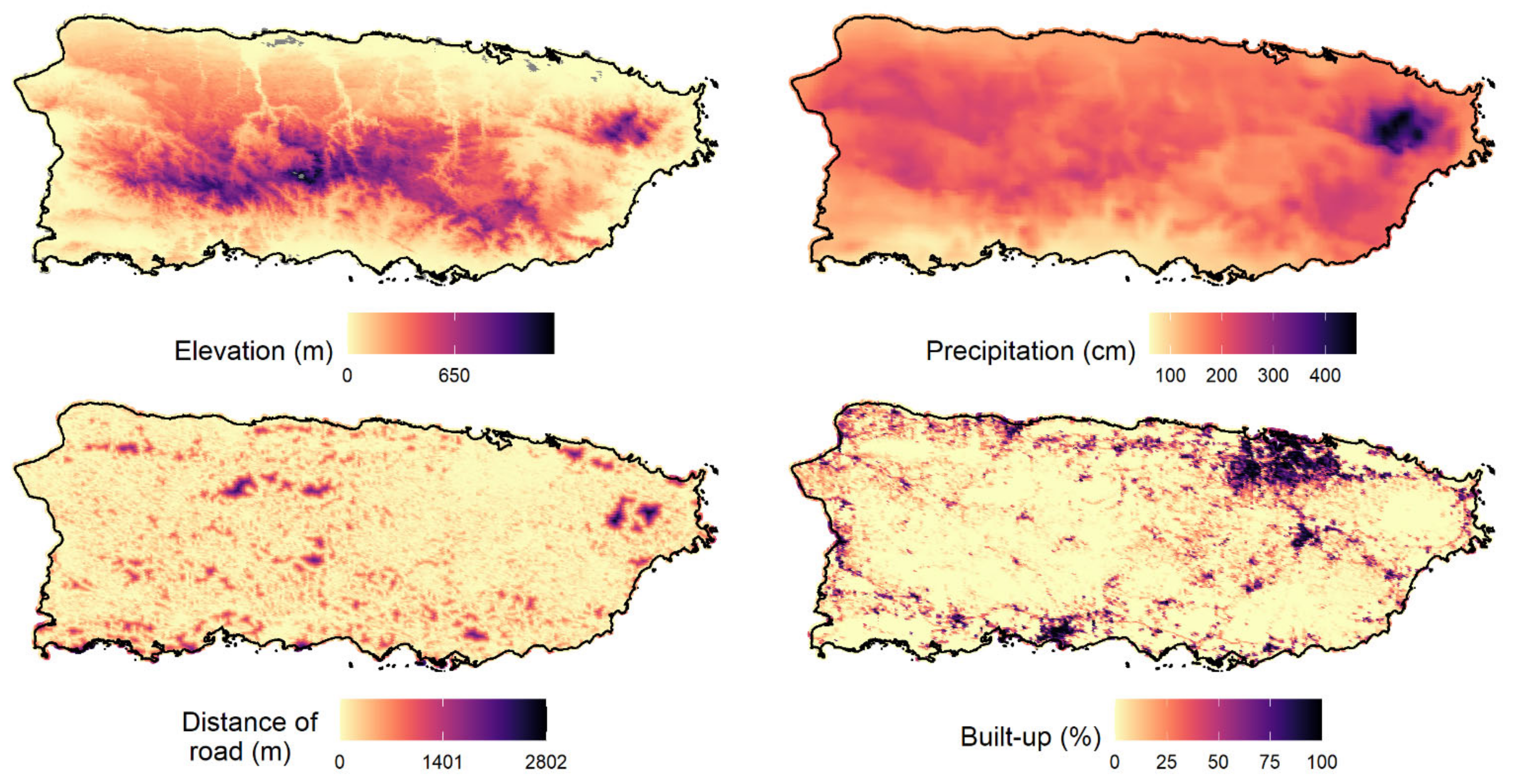
Figure A3. Maps of environmental variables across the main island of Puerto Rico. Top left: elevation (range: 0 to 1325 m); top right: mean annual precipitation (range: 71 to 433 cm); bottom left: distance of nearest road (range: 0.1 to 1864 m); bottom right: built-up proportion (range: 0 to 84%).
Remotesensing 14 04565 g0a3
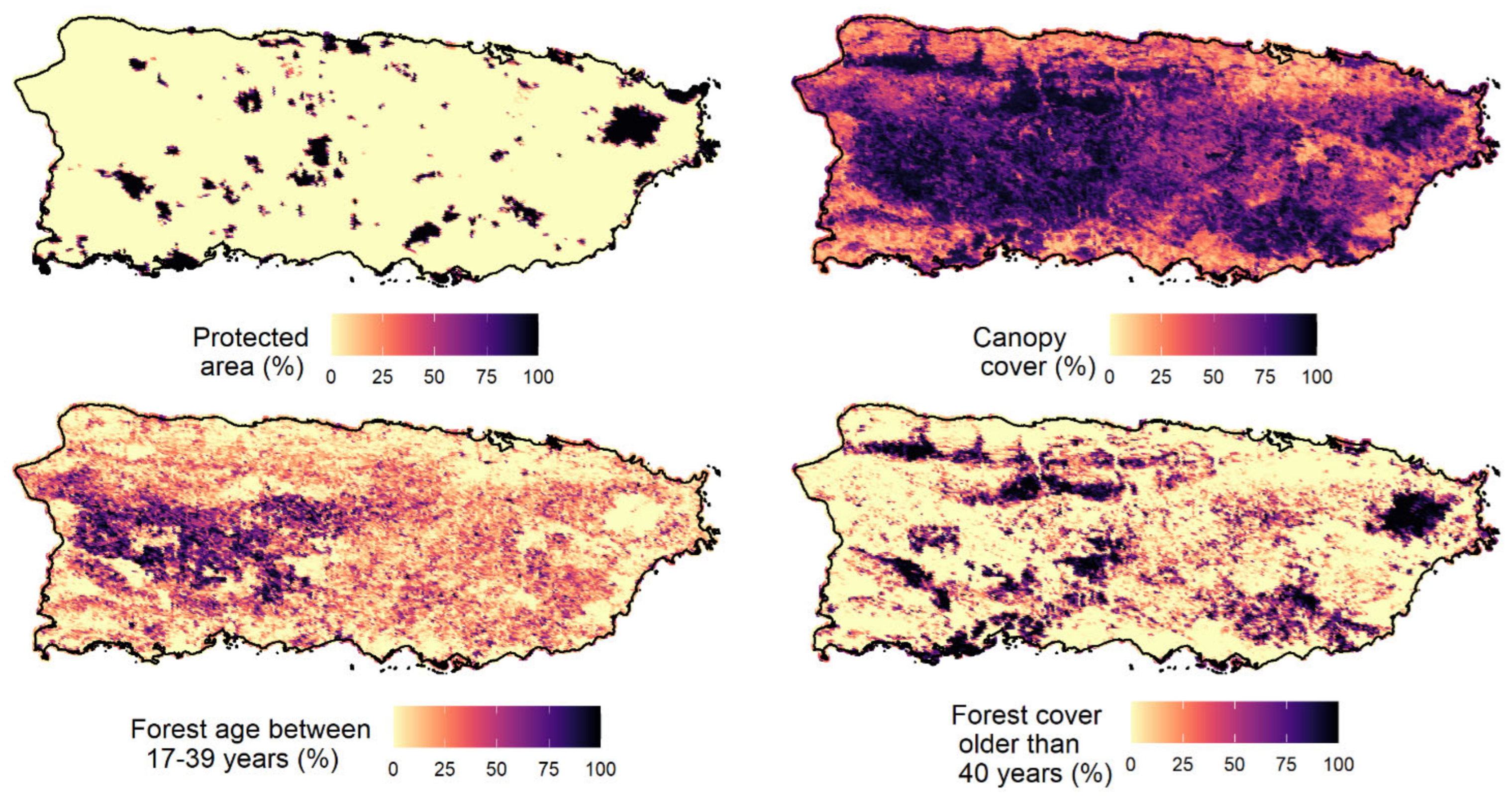
Figure A4. Maps of environmental variables across the main island of Puerto Rico. Top left: proportion of protected area (range: 0 to 100%); top right: proportion of canopy cover (range: 14 to 96%); bottom left: proportion of forest age between 34–54 years (range: 0 to 94%); bottom right: map of proportion of forest cover older than 54 years (range: 0 to 100%).
Remotesensing 14 04565 g0a4
Figure A5. Maps of environmental variables of Mona Island, Puerto Rico. Left: elevation; right: proportion of canopy cover.
Remotesensing 14 04565 g0a5
Figure A6. Maps of environmental variables across Vieques and Culebra Islands, Puerto Rico. Top left: elevation; top center: mean annual precipitation; top right: distance of the nearest road; bottom left: proportion of protected area; bottom center: proportion of canopy cover.
Remotesensing 14 04565 g0a6

Appendix C

Table A1. Table of 95 species detected (74 birds, 18 frogs, and 3 mammals) through passive acoustic monitoring (combination of manual annotations and Arbimon Pattern Matching analysis) across the 841 sampling sites in Puerto Rico. PM = Pattern Matching, indicating the species with PM analysis; IUCN = International Union for Conservation of Nature; CR = critically endangered; EN = endangered; VU = vulnerable; NT = near threatened; LC = least concern; PR = Puerto Rico main island; CU = Culebra; MO = Mona; VI = Vieques; National Red List = PRSWAP 2018; Occ = naive occupancy (proportion of sites where the species was detected); Det = detection frequency.
SpeciesIslandEndemicExoticPMIUCNNational Red List OccDet
BIRDS
Gallus gallus domesticusPR/MO/CU/VI YesYes 0.0480.006
Patagioenas leucocephalaPR/MO/VIYes YesNTVU0.0710.025
Patagioenas squamosaPR/VI YesLC 0.3340.061
Geotrygon montanaPR YesLCDD0.0110.003
Columbina passerinaPR/MO/CU/VI LC 0.0540.005
Streptopelia decaoctoPR/MO/CU YesYesLC 0.0010.000
Zenaida auritaPR/MO/CU/VI LC 0.1300.012
Zenaida asiaticaPR/MO/CU/VI LC 0.1620.021
Crotophaga aniPR/MO/CU/VI YesLC 0.1820.018
Coccyzus vieillotiPRYes YesLCLR0.2420.044
Coccyzus minorPR/MO/VI LC 0.0700.004
Chordeiles gundlachiiPR/VI YesLCDD0.0950.029
Antrostomus noctitherusPRYes YesENEN0.0830.038
Bubulcus ibisPR YesYesLC 0.0010.000
Butorides virescensPR/CU LC 0.0170.001
Aramus guaraunaPR YesLCDD0.0080.001
Pluvialis squatarolaPR/VI YesLCDD0.0380.005
Actitis maculariusPR/VI LC 0.0060.000
Tringa melanoleucaPR LC 0.0010.000
Tringa semipalmataPR LC 0.0010.000
Charadrius vociferusPR/CU/VI LC 0.0130.001
Himantopus mexicanusPR LC 0.0030.000
Fulica caribaeaPR LCVU0.0010.000
Gallinula galeataPR LC 0.0140.001
Porphyrio martinicaPR LC 0.0020.000
Rallus crepitansPR/CU LC 0.0190.002
Thalasseus maximusPR LC 0.0010.000
Larus atricillaPR/MO LC 0.0060.000
Sula sulaMO LC 0.0010.000
Buteo platypterus brunnescensPR/CU/VIYes YesLCCR0.0180.004
Buteo jamaicensisPR/CU/VI YesLC 0.1380.008
Accipiter striatus venatorPRYes YesLCCR0.0010.000
Asio flammeusPR/CU LC 0.0020.000
Gymnasio nudipesPRYes YesLC 0.3230.090
Megaceryle alcyonPR/CU/VI LC 0.0100.001
Falco sparveriusPR/MO/CU LC 0.0300.001
Todus mexicanusPRYes YesLC 0.2910.036
Melanerpes portoricensisPR/VIYes YesLCLR0.5200.108
Brotogeris versicolurusPR/VI YesYesLC 0.0140.001
Myiopsitta monachusPR YesYesLC 0.0130.001
Amazona amazonicaPR YesYesLC 0.0010.000
Amazona viridigenalisPR YesYesEN 0.0010.000
Amazona vittataPRYes YesCRCR0.0080.009
Elaenia martinicaPR/CU/VI LC 0.0580.006
Contopus latirostris blancoiPRYes YesLC 0.0170.002
Myiarchus antillarumPR/VIYes YesLC 0.4240.066
Tyrannus caudifasciatusPR/VI LC 0.0870.005
Tyrannus dominicensisPR/MO/CU/VI LC 0.2760.026
Vireo altiloquusPR/MO/VI YesLCDD0.3920.127
Vireo latimeriPRYes YesLCVU0.1300.049
Progne dominicensisPR YesLCDD0.0150.002
Margarops fuscatusPR/MO/CU/VI YesLC 0.3720.213
Turdus plumbeusPR YesLC 0.1810.027
Mimus polyglottosPR/MO/CU LC 0.0590.008
Nesospingus speculiferusPRYes YesLCDD0.0600.017
Spindalis portoricensisPRYes YesLCLR0.1710.030
Icterus portoricensisPRYes YesLCDD0.0570.005
Icterus icterusPR YesYesLC 0.1640.065
Agelaius xanthomusPR/MOYes YesENEN0.0100.003
Molothrus bonariensisPR/VI YesYesLC 0.1010.014
Quiscalus nigerPR/VI LC 0.0620.004
Setophaga americanaPR LC 0.0080.001
Setophaga angelaePRYes YesENEN0.0400.029
Setophaga petechiaPR/CU/VI YesLCVU0.0370.083
Setophaga discolorPR YesLCDD0.0240.003
Setophaga caerulescensPR YesLC 0.0050.001
Setophaga adelaidaePR/VIYes YesLCLR0.4370.140
Parkesia noveboracensisPR LC 0.0020.000
Coereba flaveolaPR/CU/VI YesLC 0.8020.229
Melopyrrha portoricensisPRYes YesLCLR0.2770.091
Melanospiza bicolorPR LC 0.0500.004
Tiaris olivaceusPR/MO LC 0.0090.000
Passer domesticusPR/CU YesYesLC 0.0060.000
Euphonia musicaPR LC 0.0020.000
FROGS
Eleutherodactylus antillensisPR/CU/VI YesLC 0.3660.107
Eleutherodactylus brittoniPR YesLCDD0.1220.083
Eleutherodactylus cochranaePR/CU/VI YesLC 0.1320.083
Eleutherodactylus cookiPRYes YesENVU0.0020.009
Eleutherodactylus coquiPR YesLC 0.3690.152
Eleutherodactylus gryllusPRYes YesCR 0.0050.006
Eleutherodactylus hedrickiPRYes YesEN 0.0130.005
Eleutherodactylus juanariveroiPRYes YesCRCR0.0010.002
Eleutherodactylus locustusPRYes YesENVU0.0050.004
Eleutherodactylus monensisMOYes YesVU 0.0030.002
Eleutherodactylus portoricensisPRYes YesENVU0.0170.059
Eleutherodactylus richmondiPR YesEN 0.0010.002
Eleutherodactylus unicolorPRYes YesCR 0.0090.023
Eleutherodactylus wightmanaePRYes YesEN 0.0470.039
Rhinella marinaPR/CU YesYesLC 0.0290.017
Osteopilus septentrionalisPR YesYesLC 0.0260.007
Leptodactylus albilabrisPR YesLC 0.1010.031
Lithobates catesbeianusPR YesYesLC 0.0190.017
MAMMALS
Canis lupus familiarisPR/CU YesYes
Capra hircusMO YesYes 0.0240.003
Equus ferus caballusPR/VI YesYes 0.0150.002

Appendix D

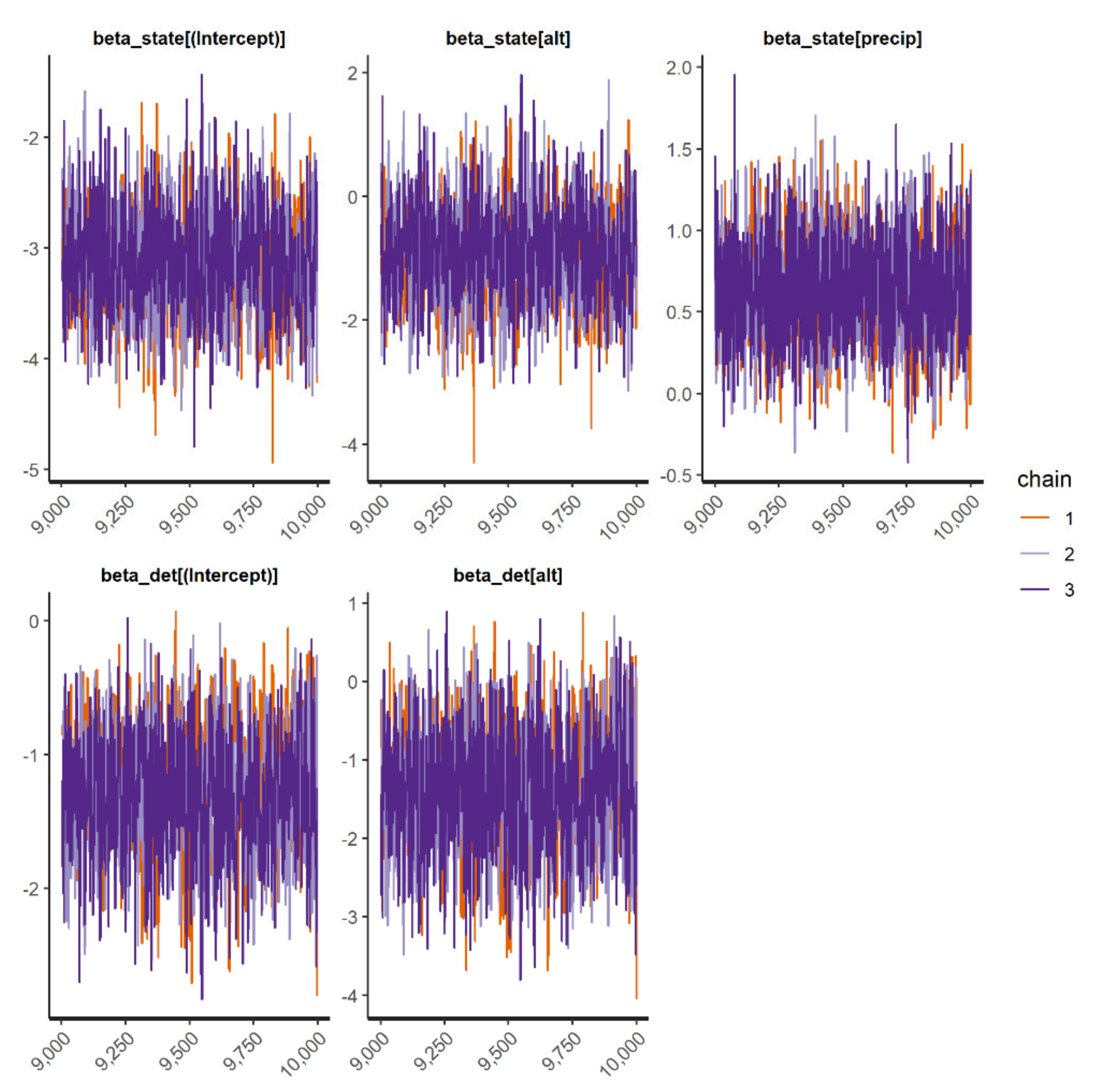
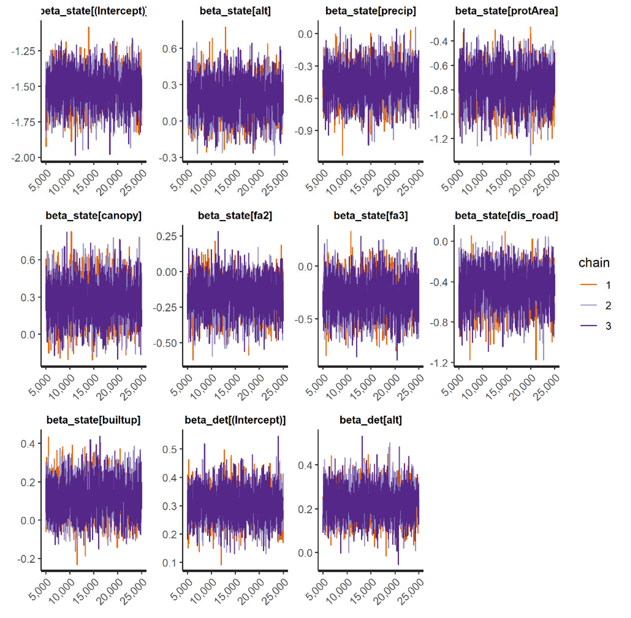
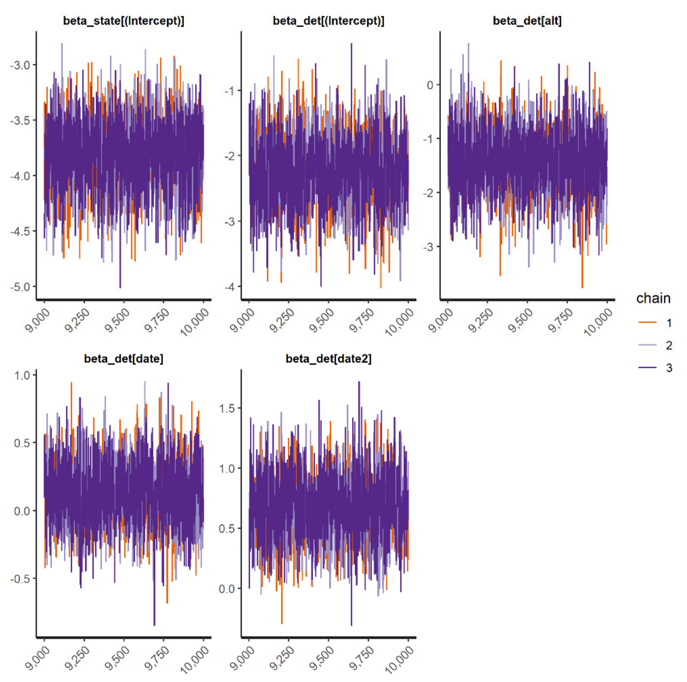
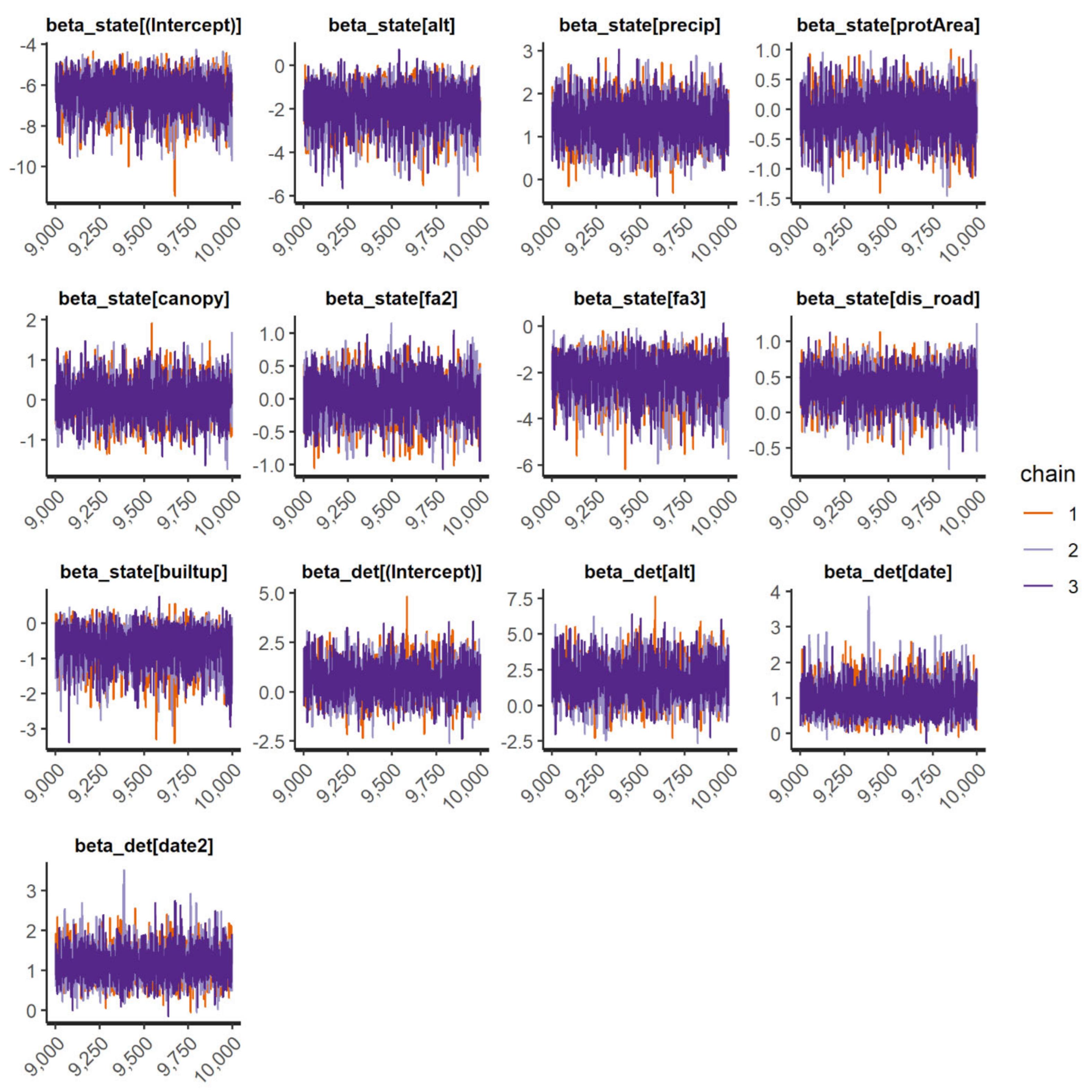
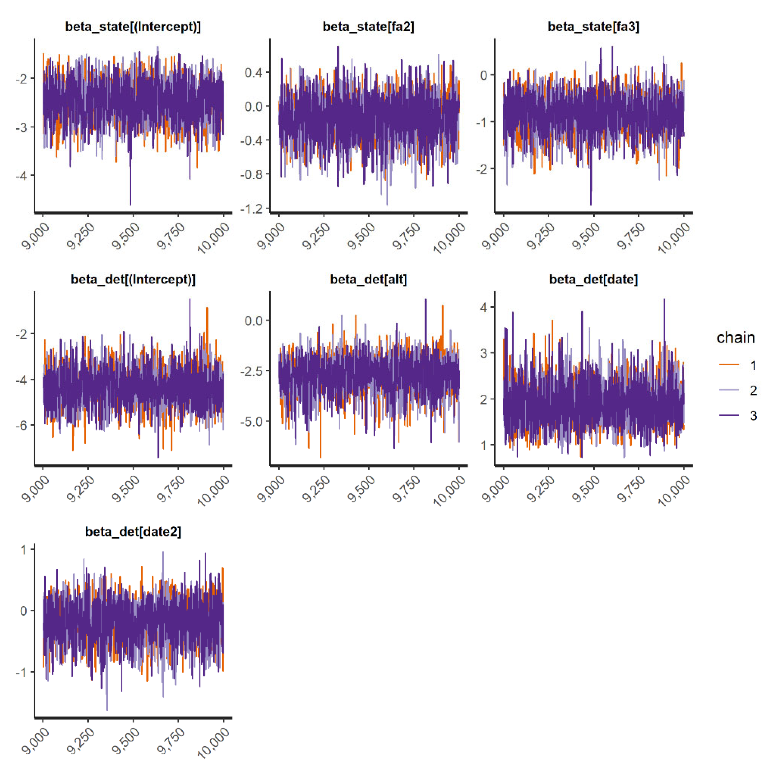
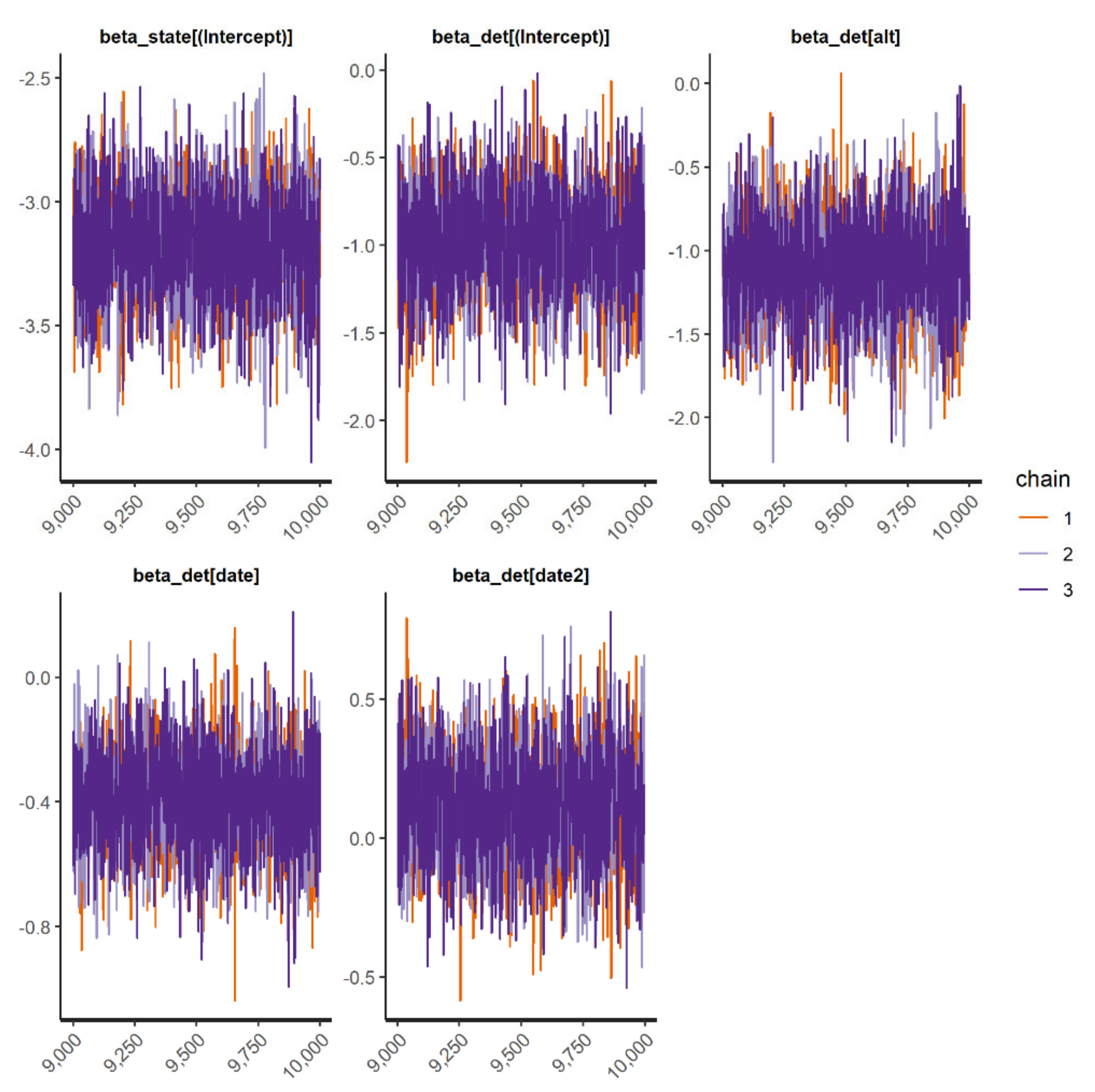
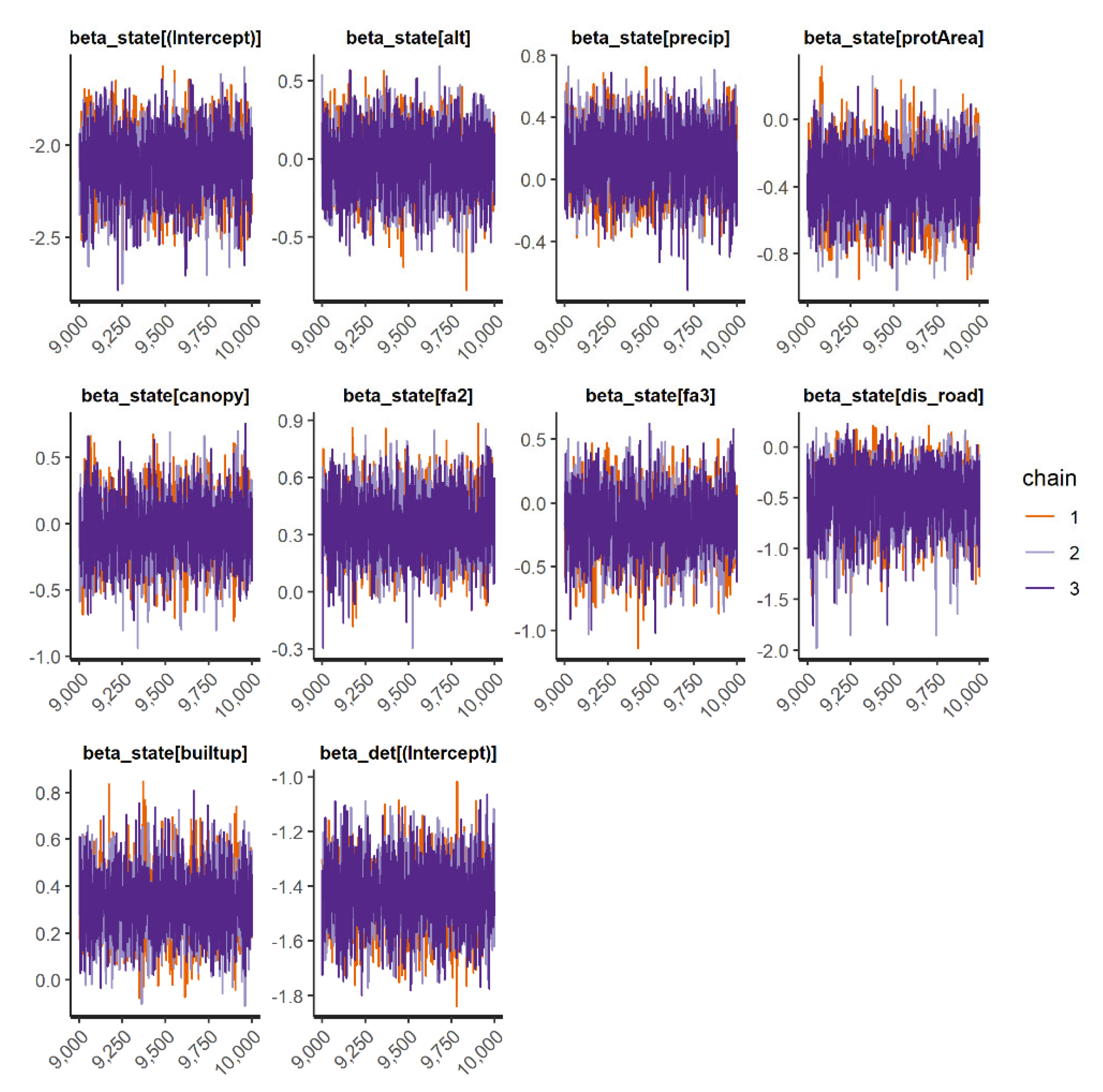
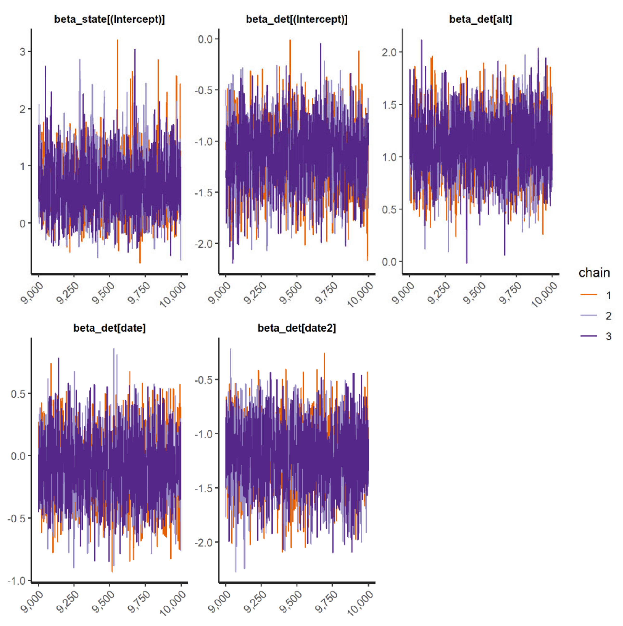
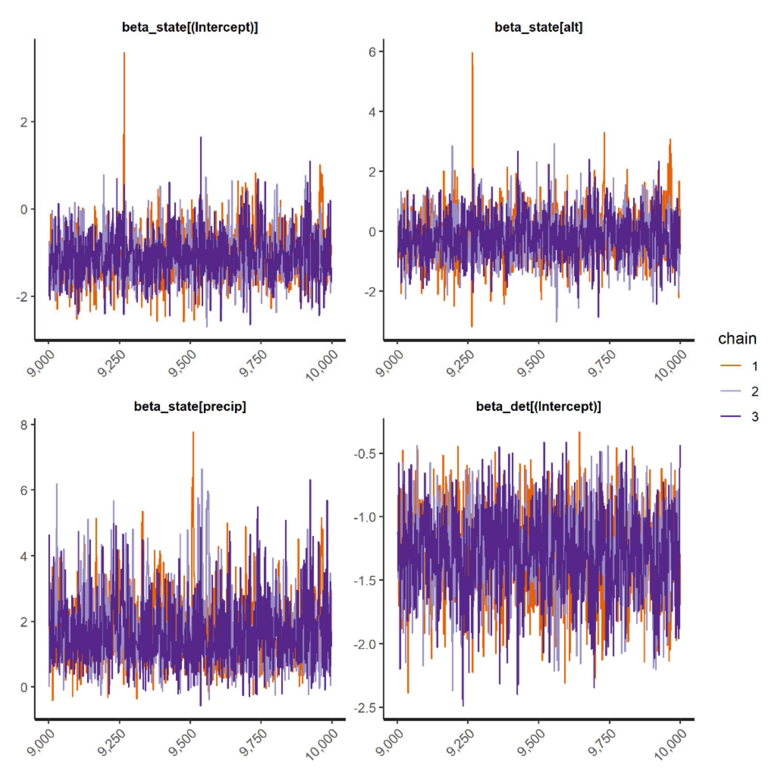
We accessed convergence and mixing across Markov chains for each parameter through visual inspection of traceplots from the best occupancy model of 11 invasive species in Puerto Rico. We used three Markov chains for all the models. When the Markov chains (characterized by different colors in the figures below) showed a random scatter around a mean value, this suggested a good mixing and convergence. The x-axis represents the number of iterations for each chain in the order in which they are drawn. The maximum number of interactions of the models varied (so the x-axis varied as well) because some models need more iterations in order for the Markov chains to achieve convergence of the parameters. The y-axis represents the estimated values of the parameter.
Figure A7. Traceplots from the best spatial occupancy model of Venezuelan troupial (Icterus icterus) in Puerto Rico: (ψ(intercept + elevation + precipitation + RSR-1000); ρ (intercept + elevation + date + date2)). Note: alt = elevation; precip = mean annual precipitation; date = Julian date (we considered Julian day 1 as the first day of a device starting to record in the field, which was 1 March 2021); date2 = square of Julian date; RSR = restricted spatial regression (threshold = 1000 m).
Remotesensing 14 04565 g0a7
Figure A8. Traceplots from the best occupancy model (ψ(intercept + elevation + precipitation); ρ (intercept + elevation)) of white-winged parakeet (Brotogeris versicolurus) in Puerto Rico. Note: alt = elevation; precip = mean annual precipitation.
Remotesensing 14 04565 g0a8
Figure A9. Traceplots from the best occupancy model of chicken (Gallus gallus domesticus) in Puerto Rico: (ψ(intercept + elevation + precipitation + protected area + canopy cover + fa2 + fa3 + distance of road + built-up + RSR-1000); ρ (intercept + elevation)). Note: alt = elevation; precip = mean annual precipitation; protArea = proportion of protected area; canopy = proportion of canopy cover; fa2 = proportion of forest cover aged between 32 and 54 years; fa3 = proportion of forest cover aged 55 years and older; dis_road = minimum distance from road; builtup = built-up proportion; RSR = restricted spatial regression (threshold = 1000 m).
Remotesensing 14 04565 g0a9
Figure A10. Traceplots from the best occupancy model (ψ(intercept); ρ (intercept + elevation + date + date2)) of shiny cowbird (Molothrus bonariensis) in Puerto Rico. Note: alt = elevation; date = Julian date (we considered Julian day 1 as the first day of a device starting to record in the field, which was 1 March 2021); date2 = square of Julian date.
Remotesensing 14 04565 g0a10
Figure A11. Traceplots from the best occupancy model (ψ(intercept); ρ (intercept + elevation + Julian day + Julian day2)) of house sparrow (Passer domesticus) in Puerto Rico. Note: alt = elevation; date = Julian date (we considered Julian day 1 as the first day of a device starting to record in the field, which was 1 March 2021); date2 = square of Julian date.
Remotesensing 14 04565 g0a11
Figure A12. Traceplots from the best occupancy model of American bullfrog (Lithobates catesbeianus) in Puerto Rico: (ψ(intercept + elevation + precipitation + protected area + canopy cover + fa2 + fa3 + distance of road + built up); ρ (intercept + elevation + date + date2)). Note: alt = elevation; precip = mean annual precipitation; protArea = proportion of protected area; canopy = proportion of canopy cover; fa2 = proportion of forest cover aged between 32 and 54 years; fa3 = proportion of forest cover aged 55 years and older; dis_road = minimum distance from road; builtup = built-up proportion; date = Julian date (we considered Julian day 1 as the first day of a device starting to record in the field, which was 1 March 2021); date2 = square of Julian date.
Remotesensing 14 04565 g0a12
Figure A13. Traceplots from the second-best occupancy model (the top-ranked model did not converge well) of Cuban tree frog (Osteopilus septentrionalis) in Puerto Rico: (ψ(intercept + fa2 + fa3); ρ (intercept + elevation + date + date2)). Note: alt = elevation; fa2 = proportion of forest cover aged between 32 and 54 years; fa3 = proportion of forest cover aged 55 years and older; date = Julian date (we considered Julian day 1 as the first day of a device starting to record in the field, which was 1 March 2021); date2 = square of Julian date.
Remotesensing 14 04565 g0a13
Figure A14. Traceplots from the best occupancy model of cane toad (Rhinella marina) in Puerto Rico: (ψ(intercept); ρ (intercept + elevation + date + date2)). Note: alt = elevation; date = Julian date (we considered Julian day 1 as the first day of a device starting to record in the field, which was 1 March 2021); date2 = square of Julian date.
Remotesensing 14 04565 g0a14
Figure A15. Traceplots from the best occupancy model of domestic dog (Canis lupus familiaris) in Puerto Rico: (ψ(intercept + elevation + precipitation + protected area + canopy cover + fa2 + fa3 + distance of road + built up); ρ (intercept + elevation)). Note: alt = elevation; precip = mean annual precipitation; protArea = proportion of protected area; canopy = proportion of canopy cover; fa2 = proportion of forest cover aged between 32 and 54 years; fa3 = proportion of forest cover aged 55 years and older; dis_road = minimum distance from road; builtup = built-up proportion.
Remotesensing 14 04565 g0a15
Figure A16. Traceplots from the best occupancy model of wild goat (Capra hircus) in Puerto Rico: (ψ(intercept); ρ (intercept + elevation + date + date2)). Note: alt = elevation; date = Julian date (we considered Julian day 1 as the first day of a device starting to record in the field, which was 1 March 2021); date2 = square of Julian date.
Remotesensing 14 04565 g0a16
Figure A17. Traceplots from the best occupancy model of feral horse (Equus ferus caballus) in Puerto Rico: (ψ(intercept + elevation + precipitation); ρ (intercept)). Note: alt = elevation; precip = mean annual precipitation.
Remotesensing 14 04565 g0a17

Appendix E

Below is the output summary from the best occupancy model used for the prediction maps for 11 invasive alien species in Puerto Rico.
Table A2. Output summary from the best model (ψ(intercept + elevation + precipitation + RSR-1000); ρ (intercept + elevation + Julian day + Julian day2)) of Venezuelan troupial (Icterus icterus) in Puerto Rico. RSR = restricted spatial regression. Runtime: 2.722 h.
CovariatesEstimatedSD2.5%97.5%n_effRhat
Occupancy (logit-scale):
Intercept−2.0340.284−2.586−1.46330191.00
Elevation−0.7540.477−1.6860.19029481.00
Precipitation−1.2870.261−1.830−0.79628361.00
RSR (tau)—1000 m0.6521.7760.0763.0703741.01
Detection (logit-scale):
Intercept−1.140.285−1.691−0.57924751.00
Elevation−1.080.450−1.937−0.20925611.00
Julian date (linear)0.580.1270.3330.82224271.00
Julian date (quadratic)−0.130.153−0.4230.17228821.00
Table A3. Output summary from the best spatial occupancy model (ψ(intercept + elevation + precipitation); ρ (intercept + elevation)) of white-winged parakeet (Brotogeris versicolurus) in Puerto Rico. Runtime: 13.692 min.
CovariatesEstimatedSD2.5%97.5%n_effRhat
Occupancy (logit-scale):
Intercept−3.1330.4614.025−2.17010211.002
Elevation−0.9250.777−2.3910.67110421.002
Precipitation0.6370.3220.0191.27218080.999
Detection (logit-scale):
Intercept−1.280.461−2.24−0.4229561.01
Elevation−1.370.780−2.960.064210191.00
Table A4. Output summary from the best spatial occupancy model (ψ(intercept + elevation + precipitation + protected area + canopy cover + fa2 + fa3 + distance of road + built up + RSR-1000); ρ (intercept + elevation)) of chicken (Gallus gallus domesticus) in Puerto Rico. Note: fa2 = proportion of forest cover aged between 32 and 54 years; fa3 = proportion of forest cover aged 55 years and older. RSR = restricted spatial regression (threshold = 1000 m). Runtime: 2.788 h.
CovariatesEstimatedSD2.5%97.5%n_effRhat
Occupancy (logit-scale):
Intercept−1.5130.122−1.764−1.28425460.999
Elevation0.1890.150−0.1110.48027141.00
Precipitation−0.4560.160−0.781−0.15626351.00
Protected area−0.7580.151−1.070−0.47921361.00
Canopy cover0.2680.159−0.0460.58227991.00
fa2−0.1760.123−0.4270.04729551.00
fa3−0.2840.172−0.6300.04523851.00
Distance of road−0.4500.185−0.840−0.11428161.00
Built up0.1170.094−0.0640.30725651.00
RSR (tau)—1000 m23.25641.8320.891138.5454031.02
Detection (logit-scale):
Intercept0.3060.0560.1970.41431181.00
Elevation0.2260.0720.0870.37031101.00
Table A5. Output summary from the best occupancy model (ψ(intercept); ρ (intercept + elevation + Julian day + Julian day2)) of shiny cowbird (Molothrus bonariensis) in Puerto Rico. Runtime: 13.118 h.
CovariatesEstimatedSD2.5%97.5%n_effRhat
Occupancy (logit-scale):
Intercept−1.80.131−2.05−1.5322441.00
Detection (logit-scale):
Intercept−1.1790.160−1.492−0.86818561.00
Elevation−0.4310.170−0.745−0.08320511.00
Julian date (linear)0.3530.1170.1260.59420111.00
Julian date (quadratic)−0.0310.125−0.2840.20318661.00
Table A6. Output summary from the best occupancy model (ψ(intercept); ρ (intercept + elevation + Julian day + Julian day2)) of house sparrow (Passer domesticus) in Puerto Rico. Runtime: 11.022 min.
CovariatesEstimatedSD2.5%97.5%n_effRhat
Occupancy (logit-scale):
Intercept−3.810.318−4.47−3.2220461
Detection (logit-scale):
Intercept−2.2250.533−3.258−1.21015371.004
Elevation−1.3920.584−2.560−0.28617041.001
Julian date (linear)0.1260.236−0.3300.59522620.999
Julian date (quadratic)0.6670.2700.1421.20319271.002
Table A7. Output summary from the best spatial occupancy model (ψ(intercept + elevation + precipitation + protected area + canopy cover + fa2 + fa3 + distance of road + built up); ρ (intercept + elevation + Julian day + Julian day2)) of American bullfrog (Lithobates catesbeianus) in Puerto Rico. Note: fa2 = proportion of forest cover aged between 32 and 54 years; fa3 = proportion of forest cover aged 55 years and older. Runtime: 40.292 min.
CovariatesEstimatedSD2.5%97.5%n_effRhat
Occupancy (logit-scale):
Intercept−6.4540.936−8.477−4.88913431.001
Elevation−1.8460.953−4.113−0.33421551.001
Precipitation1.3320.4900.4132.28128091.000
Protected area−0.0980.366−0.8520.58233760.999
Canopy cover0.0150.478−0.9310.96830711.000
fa20.0170.317−0.610.62631100.999
fa3−2.2670.888−4.267−0.79918351.001
Distance of road0.3490.262−0.1970.84131091.000
Built up−0.6950.546−1.9460.17624020.999
Detection (logit-scale):
Intercept0.5720.903−1.1152.4524260.999
Elevation1.7551.345−0.7644.5625031.000
Julian date (linear)0.9790.4750.2252.0917660.999
Julian date (quadratic)1.1700.4280.4162.1117381.000
Table A8. Output summary from the second-best occupancy model (ψ(fa2 + fa3); ρ (intercept + elevation + Julian day + Julian day2)) of Cuban tree frog (Osteopilus septentrionalis) in Puerto Rico (the top-ranked model did not converge well). Note: fa2 = proportion of forest cover aged between 32 and 54 years; fa3 = proportion of forest cover aged 55 years and older. Runtime: 29.712 min.
CovariatesEstimatedSD2.5%97.5%n_effRhat
Occupancy (logit-scale):
Intercept−2.4580.400−3.268−1.72017831
fa2−0.1440.254−0.6740.34027611
fa3−0.8310.408−1.672−0.08520851
Detection (logit-scale):
Intercept−4.3640.804−5.946−2.75117151
Elevation−2.7840.915−4.817−1.18118331
Julian date (linear)1.9190.4661.1062.96018621
Julian date (quadratic)−0.2020.337−0.8910.42221181
Table A9. Output summary from the best occupancy model (ψ(intercept); ρ (intercept + elevation + Julian day + Julian day2)) of cane toad (Rhinella marina) in Puerto Rico. Runtime: 9.981 min.
CovariatesEstimatedSD2.5%97.5%n_effRhat
Occupancy (logit-scale):
Intercept−3.170.217−3.6−2.7725301.00
Detection (logit-scale):
Intercept−0.9830.300−1.609−0.41714481.00
Elevation−1.1090.311−1.712−0.49125611.00
Julian date (linear)−0.3950.160−0.711−0.08525381.00
Julian date (quadratic)0.1130.201−0.2740.50616261.00
Table A10. Output summary from the best spatial occupancy model (ψ(intercept + elevation + precipitation + protected area + canopy cover + fa2 + fa3 + distance of road + built up); ρ (intercept)) of domestic dog (Canis lupus familiaris) in Puerto Rico. Note: fa2 = proportion of forest cover aged between 32 and 54 years; fa3 = proportion of forest cover aged 55 years and older. Runtime: 11.735 min.
CovariatesEstimatedSD2.5%97.5%n_effRhat
Occupancy (logit-scale):
Intercept−2.1060.175−2.472−1.7752092 1.00
Elevation−0.0180.197−0.4110.35729751.00
Precipitation0.1320.199−0.2570.51528691.00
Protected area−0.3720.192−0.757−0.00629481.00
Canopy cover−0.0500.233−0.5140.40622641.00
fa20.3560.1620.0470.67125381.00
fa3−0.1540.246−0.6430.33623201.00
Distance of road−0.4990.304−1.1380.01521411.00
Built up0.3260.1370.0680.60528341.00
Detection (logit-scale):
Intercept−1.430.12−1.67−1.231590.999
Table A11. Output summary from the best occupancy model (ψ(intercept); ρ (intercept + Julian day + Julian day2)) of wild goat (Capra hircus) in Puerto Rico. Runtime: 49.586 s.
CovariatesEstimatedSD2.5%97.5%n_effRhat
Occupancy (logit-scale):
Intercept0.6880.504−0.1821.7317751.00
Detection (logit-scale):
Intercept−1.1470.315−1.794−0.53916591.002
Elevation1.1000.2960.5451.66620831.001
Julian date (linear)−0.0870.264−0.6010.43529250.999
Julian date (quadratic)−1.1970.307−1.826−0.64622331.00
Table A12. Output summary from the best spatial occupancy model (ψ(intercept + elevation + precipitation); ρ (intercept)) of feral horse (Equus ferus caballus) in Puerto Rico. Runtime: 41.425 s.
CovariatesEstimatedSD2.5%97.5%n_effRhat
Occupancy (logit-scale):
Intercept−1.0680.551−2.080.11511921.00
Elevation−0.1630.794−1.641.46112931.00
Precipitation1.7301.0700.164.3548481.00
Detection (logit-scale):
Intercept−1.280.338−1.99−0.64912471.00

Appendix F

Figure A18. Prediction maps using the top-ranked model (mean expected occupancy probability) with the model prediction uncertainty (standard deviation) for the invasive alien species found during passive acoustic monitoring across Puerto Rico. When the top-ranked model of the species was the null model for occupancy or did not converge well, we used the model that ranked second-best to draw the prediction maps (i.e., for Molothrus bonariensis, Osteopilus septentrionalis, Rhinella marina, and Capra hircus), and as such, we highlight that these predictions should be interpreted with caution because there was a high uncertainty associated with them. The circles represent the sampling sites where the species were detected by the AudioMoth devices. The prediction for wild goat was made for Mona Island, the prediction for feral horse was made for Vieques island, and the predictions for the other species were made for the main island of Puerto Rico.
Remotesensing 14 04565 g0a18aRemotesensing 14 04565 g0a18bRemotesensing 14 04565 g0a18c

Appendix G

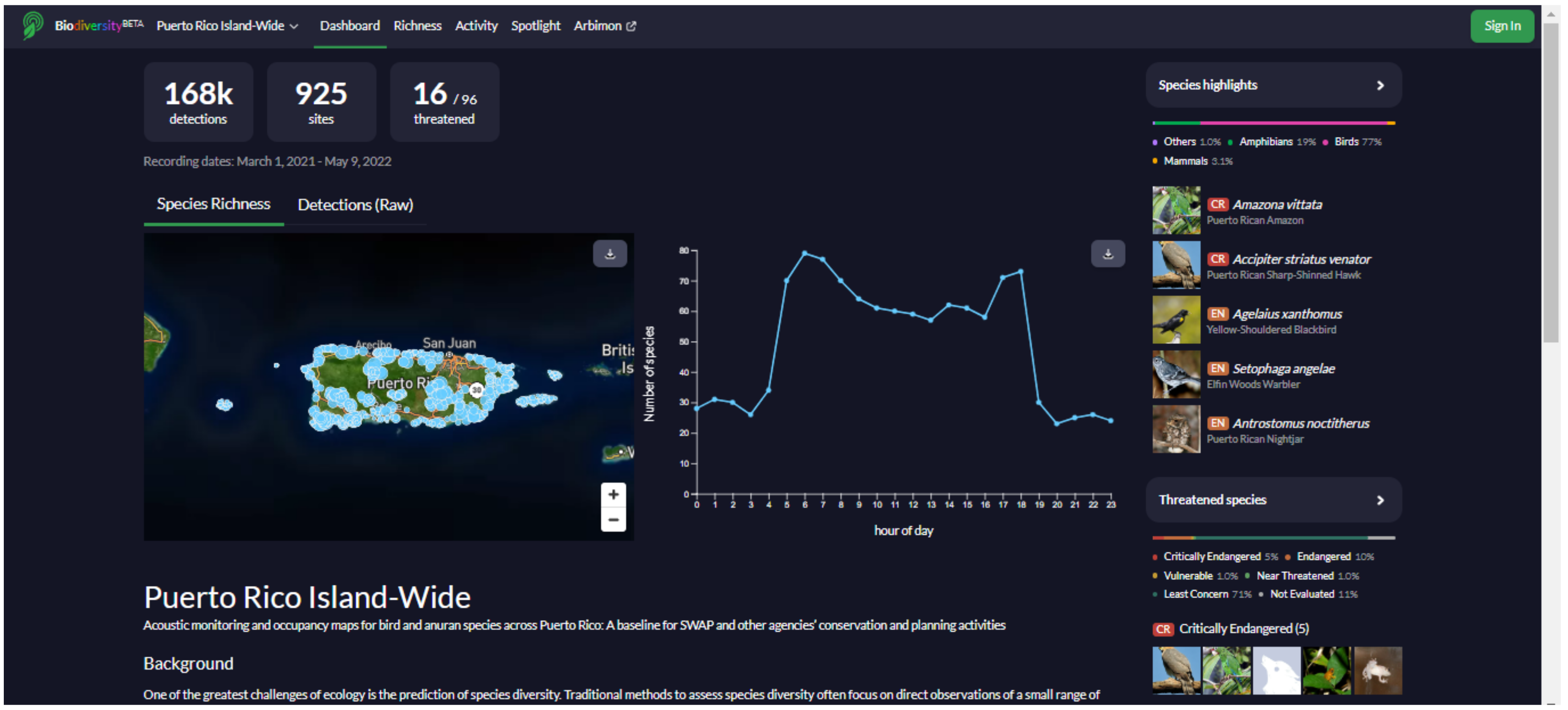
We created a biodiversity insight page as a new feature of Arbimon web-based platform for use by government agencies (e.g., Departamento de Recursos Naturales y Ambientales (DRNA), U.S. Fish and Wildlife Service), and the general public (e.g., educators and birdwatchers). The platform provides access to the main results of this study and information on the calls, behavior, and biology of the species detected in the ARU (https://bio.rfcx.org/puerto-rico-island-wide (accessed on 14 June 2022)). The main features of this page include information on the vocalizations, distributions, and ecologies of most bird and anuran species in Puerto Rico. The page also includes a searchable database that contains the detection data, presence/absence maps, and occupancy maps for the birds and anurans detected at the 841 sampling sites. All maps, plots, and data used to generate the figures can be downloaded. Since the project is still in progress, the data on the page are constantly being updated as more data are validated.
Figure A19. Dashboard: This page presents an overview of the project, including background information, objectives, funding, and stakeholders. General results are also presented, such as the total number of detections, sampling sites, species detected, and the number of species in each threat category according to the International Union for Conservation of Nature (IUCN). This page also features a map with all sampling sites and the number of species detected at each site.
Remotesensing 14 04565 g0a19
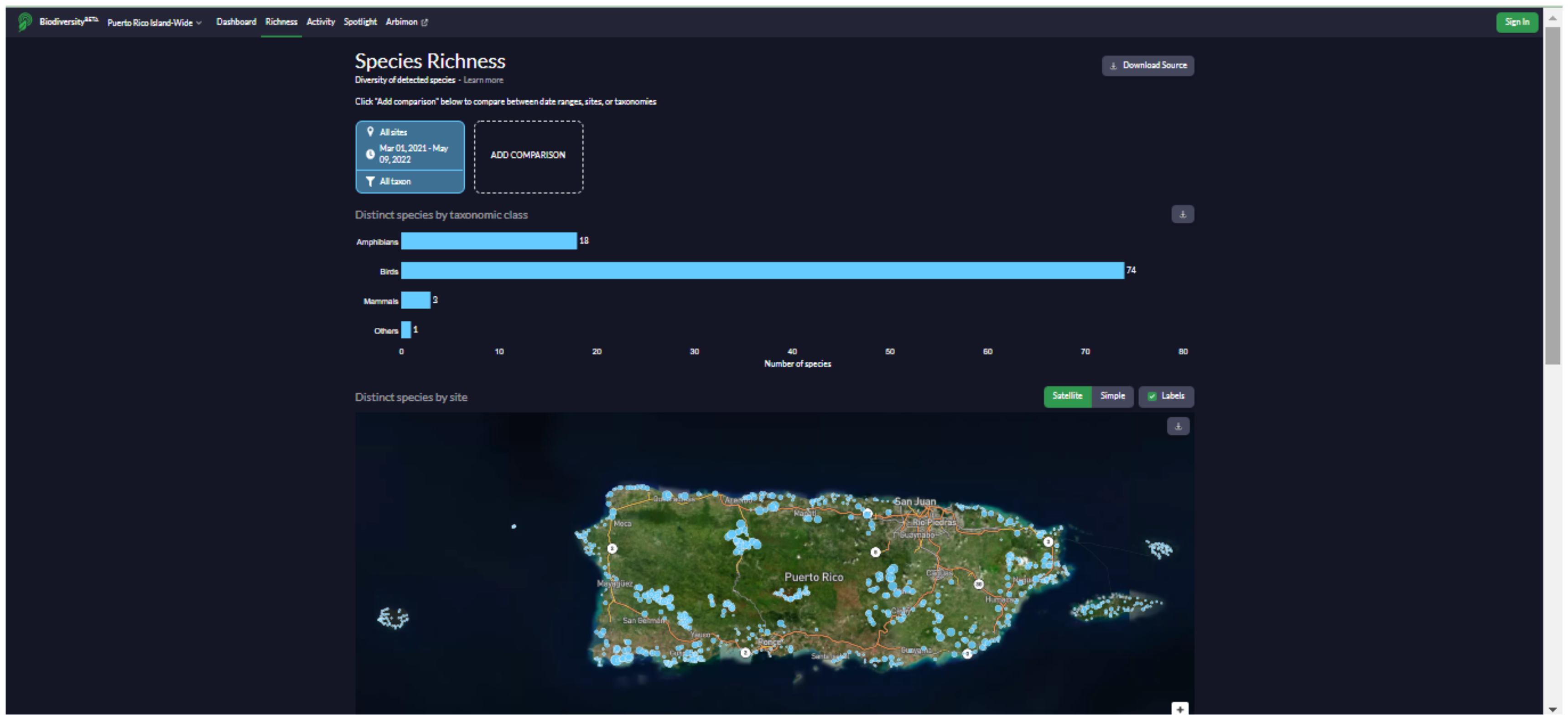
Figure A20. Species Richness: This page presents the results of the number of species detected and allows for exploration of those data in greater detail. The data are presented as a bar graph with aggregated results that can be filtered by region/site, date, and taxonomic group. Below the bar graph is an accompanying map depicting species richness in the selected sites; the point size reflects the number of species detected at each location. Below the map is a graph displaying the number of species according to time of day, day of the week, month, or date.
Remotesensing 14 04565 g0a20
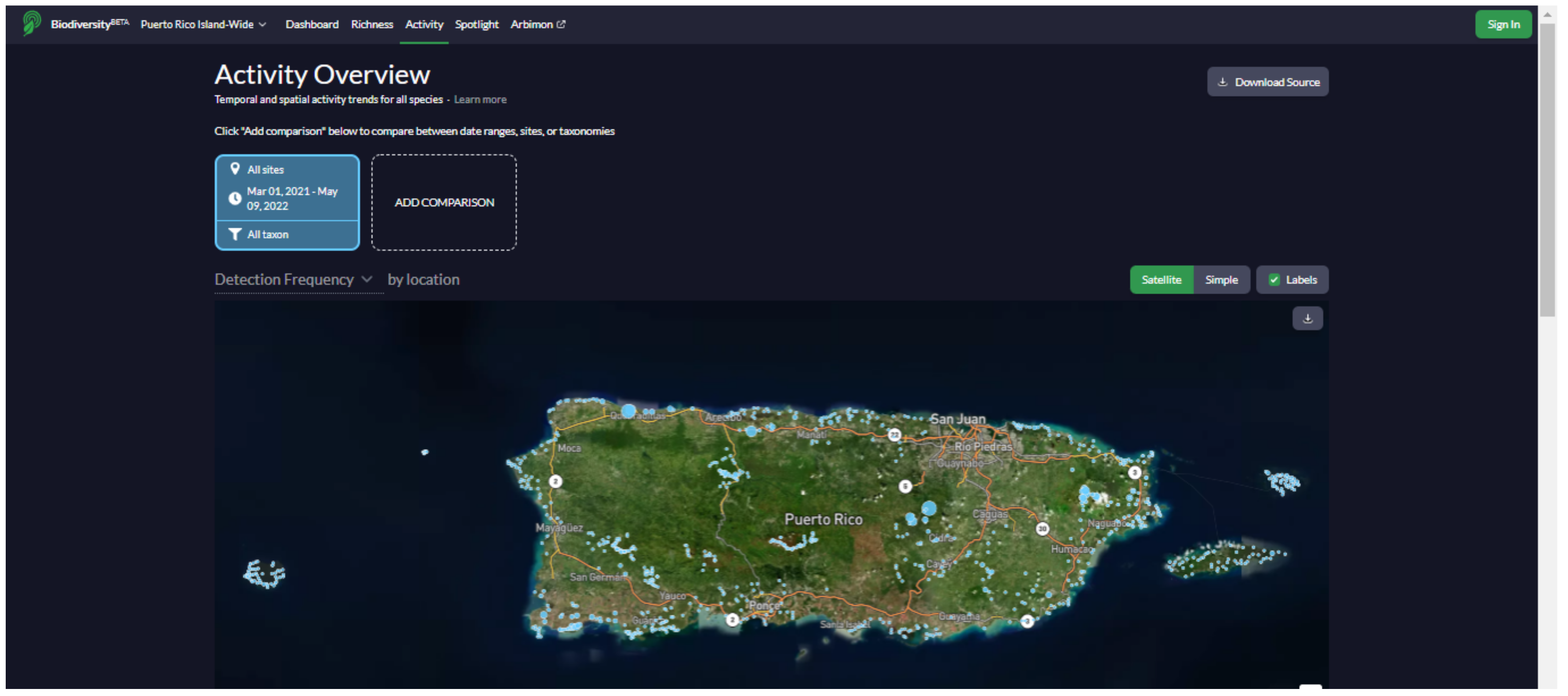
Figure A21. Activity Overview: This page offers an overview of temporal and spatial vocal activity patterns. It can be used to summarize detection frequency, number of raw detections, or naive occupancy results (i.e., proportion of occupied sites), with a focus given to general patterns at the community level. As with the Richness page, the user can use the filters to select results from taxonomic groups, sampling sites, or specific periods and visualize the results in a map or graphs that present the results according to the hour, day of the week, or month.
Remotesensing 14 04565 g0a21
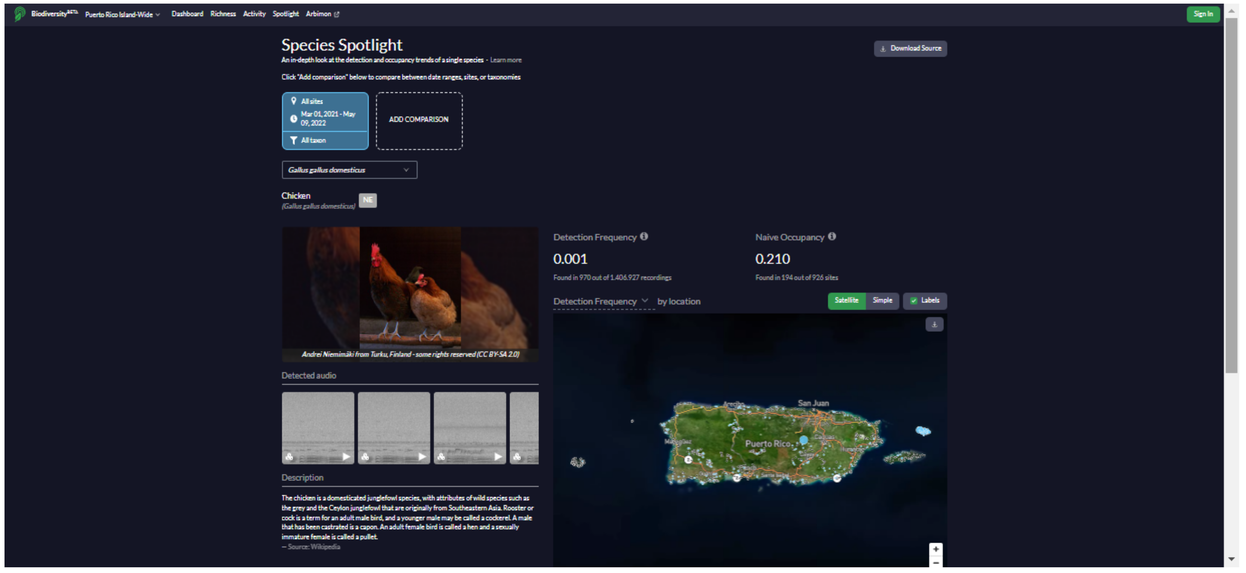
Figure A22. Spotlight: This page offers an in-depth look at the raw detection and occupancy of individual species. On this page, the user can select the species that were detected in the project data using either the scientific or common name. Basic information about the species, photo, call example, population status according to IUCN, detection frequency, and naive occupancy values are presented. The first map shows the detection results by site and allows for filtering by detection frequency, the number of detections (raw), and naive occupancy (i.e., proportion of occupied sites). A second map, when available for the species, shows the predicted occupancy (i.e., probability of occupancy) in Puerto Rico. In addition, a graph displays either detection frequency or the number of detections results according to the hour, day of the week, or month. Like the Richness and Activity pages, the data set can be subset by selecting one or more sampling sites or sampling periods.
Remotesensing 14 04565 g0a22

Appendix H

Figure A23. Map of sites where the species with low raw detections were found (<10 sites detected). The light-green polygons represent protected areas.
Remotesensing 14 04565 g0a23

References

  1. World Wide Fund for Nature. WWF Living Planet Report 2020—Bending the Curve of Biodiversity Loss; WWF: Gland, Switzerland, 2020; Volume 159. [Google Scholar]
  2. Simberloff, D. Invasive Species: What Everyone Needs to Know; Oxford University Press: Oxford, UK, 2013. [Google Scholar]
  3. Marbuah, G.; Gren, I.-M.; McKie, B. Economics of harmful invasive species: A review. Diversity 2014, 6, 500–523. [Google Scholar] [CrossRef]
  4. Dueñas, M.A.; Hemming, D.J.; Roberts, A.; Diaz-Soltero, H. The threat of invasive species to IUCN-listed critically endangered species: A systematic review. Glob. Ecol. Conserv. 2021, 26, e01476. [Google Scholar] [CrossRef]
  5. Pyšek, P.; Hulme, P.E.; Simberloff, D.; Bacher, S.; Blackburn, T.M.; Carlton, J.T.; Dawson, W.; Essl, F.; Foxcroft, L.C.; Genovesi, P.; et al. Scientists’ warning on invasive alien species. Biol. Rev. 2020, 95, 1511–1534. [Google Scholar] [CrossRef] [PubMed]
  6. Bellard, C.; Thuiller, W.; Leroy, B.; Genovesi, P.; Bakkenes, M.; Courchamp, F. Will climate change promote future invasions? Glob. Chang. Biol. 2013, 19, 3740–3748. [Google Scholar] [CrossRef] [PubMed]
  7. Tershy, B.R.; Shen, K.W.; Newton, K.M.; Holmes, N.D.; Croll, D.A. The importance of islands for the protection of biological and linguistic diversity. Bioscience 2015, 65, 592–597. [Google Scholar] [CrossRef]
  8. Dawson, W.; Moser, D.; Van Kleunen, M.; Kreft, H.; Pergl, J.; Pyšek, P.; Weigelt, P.; Winter, M.; Lenzner, B.; Blackburn, T.M.; et al. Global hotspots and correlates of alien species richness across taxonomic groups. Nat. Ecol. Evol. 2017, 1, 186. [Google Scholar] [CrossRef]
  9. Moore, J.H.; Palmeirim, A.F.; Peres, C.A.; Ngoprasert, D.; Gibson, L. Invasive rat drives complete collapse of native small mammal communities in insular forest fragments. Curr. Biol. 2022, 32, 2997–3004.e2. [Google Scholar] [CrossRef]
  10. Groom, Q.J.; Adriaens, T.; Desmet, P.; Simpson, A.; De Wever, A.; Bazos, I.; Cardoso, A.C.; Charles, L.; Christopoulou, A.; Gazda, A.; et al. Seven recommendations to make your invasive alien species data more useful. Front. Appl. Math. Stat. 2017, 3, 13. [Google Scholar] [CrossRef]
  11. Reaser, J.K.; Simpson, A.; Guala, G.F.; Morisette, J.T.; Fuller, P. Envisioning a national invasive species information framework. Biol. Invasions 2020, 22, 21–36. [Google Scholar] [CrossRef]
  12. Caffrey, J.M.; Baars, J.R.; Barbour, J.H.; Boets, P.; Boon, P.; Davenport, K.; Dick, J.T.A.; Early, J.; Edsman, L.; Gallagher, C.; et al. Tackling invasive alien species in Europe: The top 20 issues. Manag. Biol. Invasions 2014, 5, 1–20. [Google Scholar] [CrossRef] [Green Version]
  13. Rohde, S.; Schupp, P.J.; Markert, A.; Wehrmann, A. Only half of the truth: Managing invasive alien species by rapid assessment. Ocean Coast. Manag. 2017, 146, 26–35. [Google Scholar] [CrossRef]
  14. Yemshanov, D.; Haight, R.G.; Koch, F.H.; Venette, R.C.; Swystun, T.; Fournier, R.E.; Marcotte, M.; Chen, Y.; Turgeon, J.J. Optimizing surveillance strategies for early detection of invasive alien species. Ecol. Econ. 2019, 162, 87–99. [Google Scholar] [CrossRef]
  15. Turner, W. Sensing biodiversity. Science 2014, 346, 301–302. [Google Scholar] [CrossRef] [PubMed]
  16. Turner, W.; Spector, S.; Gardiner, N.; Fladeland, M.; Sterling, E.; Steininger, M. Remote sensing for biodiversity science and conservation. Trends Ecol. Evol. 2003, 18, 306–314. [Google Scholar] [CrossRef]
  17. Reddy, C.S. Remote sensing of biodiversity: What to measure and monitor from space to species? Biodivers. Conserv. 2021, 30, 2617–2631. [Google Scholar] [CrossRef]
  18. Huang, C.; Asner, G.P. Applications of remote sensing to alien invasive plant studies. Sensors 2009, 9, 4869–4889. [Google Scholar] [CrossRef]
  19. Rajah, P.; Odindi, J.; Mutanga, O.; Kiala, Z. The utility of Sentinel-2 Vegetation Indices (VIs) and Sentinel-1 Synthetic Aperture Radar (SAR) for invasive alien species detection and mapping. Nat. Conserv. 2019, 35, 41–61. [Google Scholar] [CrossRef]
  20. Royimani, L.; Mutanga, O.; Odindi, J.; Dube, T.; Matongera, T.N. Advancements in satellite remote sensing for mapping and monitoring of alien invasive plant species (AIPs). Phys. Chem. Earth 2019, 112, 237–245. [Google Scholar] [CrossRef]
  21. Dejean, T.; Valentini, A.; Miquel, C.; Taberlet, P.; Bellemain, E.; Miaud, C. Improved detection of an alien invasive species through environmental DNA barcoding: The example of the American bullfrog Lithobates catesbeianus. J. Appl. Ecol. 2012, 49, 953–959. [Google Scholar] [CrossRef]
  22. Geerts, A.N.; Boets, P.; Van den Heede, S.; Goethals, P.; Van der Heyden, C. A search for standardized protocols to detect alien invasive crayfish based on environmental DNA (eDNA): A lab and field evaluation. Ecol. Indic. 2018, 84, 564–572. [Google Scholar] [CrossRef]
  23. Aide, T.M.; Corrada-Bravo, C.; Campos-Cerqueira, M.; Milan, C.; Vega, G.; Alvarez, R. Real-time bioacoustics monitoring and automated species identification. PeerJ 2013, 1, 1–19. [Google Scholar] [CrossRef] [PubMed]
  24. Corrada-Bravo, C.J.; Berríos, R.Á.; Aide, T.M. Species-specific audio detection: A comparison of three template-based detection algorithms using random forests. PeerJ Comput. Sci. 2017, 3, e113. [Google Scholar] [CrossRef]
  25. Xie, J.; Towsey, M.; Zhu, M.; Zhang, J.; Roe, P. An intelligent system for estimating frog community calling activity and species richness. Ecol. Indic. 2017, 82, 13–22. [Google Scholar] [CrossRef]
  26. Hill, A.P.; Prince, P.; Covarrubias, E.P.; Doncaster, C.P.; Snaddon, J.L.; Rogers, A. AudioMoth: Evaluation of a smart open acoustic device for monitoring biodiversity and the environment. Methods Ecol. Evol. 2018, 9, 1199–1211. [Google Scholar] [CrossRef]
  27. Sugai, L.S.M.; Silva, T.S.F.; Ribeiro, J.W.; Llusia, D. Terrestrial passive acoustic monitoring: Review and perspectives. Bioscience 2019, 69, 15–25. [Google Scholar] [CrossRef]
  28. Zwerts, J.A.; Stephenson, P.J.; Maisels, F.; Rowcliffe, M.; Astaras, C.; Jansen, P.A.; van der Waarde, J.; Sterck, L.E.H.M.; Verweij, P.A.; Bruce, T.; et al. Methods for wildlife monitoring in tropical forests: Comparing human observations, camera traps, and passive acoustic sensors. Conserv. Sci. Pract. 2021, 3, e568. [Google Scholar] [CrossRef]
  29. Deichmann, J.L.; Acevedo-Charry, O.; Barclay, L.; Burivalova, Z.; Campos-Cerqueira, M.; D’Horta, F.; Game, E.T.; Gottesman, B.L.; Hart, P.J.; Kalan, A.K.; et al. It’s time to listen: There is much to be learned from the sounds of tropical ecosystems. Biotropica 2018, 50, 713–718. [Google Scholar] [CrossRef]
  30. Sugai, L.S.M.; Desjonquères, C.; Silva, T.S.F.; Llusia, D. A roadmap for survey designs in terrestrial acoustic monitoring. Remote Sens. Ecol. Conserv. 2020, 6, 220–235. [Google Scholar] [CrossRef]
  31. Gibb, R.; Browning, E.; Glover-Kapfer, P.; Jones, K.E. Emerging opportunities and challenges for passive acoustics in ecological assessment and monitoring. Methods Ecol. Evol. 2019, 10, 169–185. [Google Scholar] [CrossRef]
  32. Juanes, F. Visual and acoustic sensors for early detection of biological invasions: Current uses and future potential. J. Nat. Conserv. 2018, 42, 7–11. [Google Scholar] [CrossRef]
  33. Larson, E.R.; Graham, B.M.; Achury, R.; Coon, J.J.; Daniels, M.K.; Gambrell, D.K.; Jonasen, K.L.; King, G.D.; LaRacuente, N.; Perrin-Stowe, T.I.N.; et al. From eDNA to citizen science: Emerging tools for the early detection of invasive species. Front. Ecol. Environ. 2020, 18, 194–202. [Google Scholar] [CrossRef]
  34. Rountree, R.A.; Juanes, F. Potential of passive acoustic recording for monitoring invasive species: Freshwater drum invasion of the Hudson River via the New York canal system. Biol. Invasions 2017, 19, 2075–2088. [Google Scholar] [CrossRef]
  35. Brodie, S.; Yasumiba, K.; Towsey, M.; Roe, P.; Schwarzkopf, L. Acoustic monitoring reveals year-round calling by invasive toads in tropical Australia. Bioacoustics 2021, 30, 125–141. [Google Scholar] [CrossRef]
  36. Darras, K.; Batáry, P.; Furnas, B.J.; Grass, I.; Mulyani, Y.A.; Tscharntke, T. Autonomous sound recording outperforms human observation for sampling birds: A systematic map and user guide. Ecol. Appl. 2019, 29, e01954. [Google Scholar] [CrossRef]
  37. Browning, E.; Gibb, R.; Glover-Kapfer, P.; Jones, K.E. Passive Acoustic Monitoring in Ecology and Conservation; WWF: Gland, Switzerland, 2017; Volume 2. [Google Scholar]
  38. Campos-Cerqueira, M.; Aide, T.M. Improving distribution data of threatened species by combining acoustic monitoring and occupancy modelling. Methods Ecol. Evol. 2016, 7, 1340–1348. [Google Scholar] [CrossRef]
  39. Ribeiro, J.W.; Sugai, L.S.M.; Campos-Cerqueira, M. Passive acoustic monitoring as a complementary strategy to assess biodiversity in the Brazilian Amazonia. Biodivers. Conserv. 2017, 26, 2999–3002. [Google Scholar] [CrossRef]
  40. Campos-Cerqueira, M.; Arendt, W.J.; Wunderle, J.M.; Aide, T.M. Have bird distributions shifted along an elevational gradient on a tropical mountain? Ecol. Evol. 2017, 7, 9914–9924. [Google Scholar] [CrossRef]
  41. Muha, T.P.; Rodríguez-Rey, M.; Rolla, M.; Tricarico, E. Using environmental DNA to improve species distribution models for freshwater invaders. Front. Ecol. Evol. 2017, 5, 158. [Google Scholar] [CrossRef]
  42. Wood, C.M.; Popescu, V.D.; Klinck, H.; Keane, J.J.; Gutiérrez, R.J.; Sawyer, S.C.; Peery, M.Z. Detecting small changes in populations at landscape scales: A bioacoustic site-occupancy framework. Ecol. Indic. 2019, 98, 492–507. [Google Scholar] [CrossRef]
  43. Myers, N.; Mittermeier, R.A.; Mittermeier, C.G.; da Fonseca, G.A.B.; Kent, J. Biodiversity hotspots for conservation priorities. Nature 2000, 403, 853–858. [Google Scholar] [CrossRef]
  44. Finch, D.M.; Pearson, D.; Wunderle, J.; Arendt, W. Terrestrial animals as invasive species and as species at risk from invasions. In A Dynamic Invasive Species Research Vision: Opportunities and Priorities 2009-29; Dix, M.E., Britton, K., Eds.; U.S. Department of Agriculture, Forest Service Research and Development: Washington, DC, USA, 2009; pp. 43–54. [Google Scholar]
  45. Zimmerman, J.K.; Rojas-Sandoval, J.; Shiels, A.B. Invasive species in Puerto Rico: The view from El Yunque. Front. Ecol. Evol. 2021, 9, 640121. [Google Scholar] [CrossRef]
  46. LeBien, J.; Zhong, M.; Campos-Cerqueira, M.; Velev, J.P.; Dodhia, R.; Ferres, J.L.; Aide, T.M. A pipeline for identification of bird and frog species in tropical soundscape recordings using a convolutional neural network. Ecol. Inform. 2020, 59, 101113. [Google Scholar] [CrossRef]
  47. Campos-Cerqueira, M.; Aide, T.M. Impacts of a drought and hurricane on tropical bird and frog distributions. Ecosphere 2021, 12, e03352. [Google Scholar] [CrossRef]
  48. Campos-Cerqueira, M.; Terando, A.J.; Murray, B.A.; Collazo, J.A.; Aide, T.M. Climate change is creating a mismatch between protected areas and suitable habitats for frogs and birds in Puerto Rico. Biodivers. Conserv. 2021, 30, 3509–3528. [Google Scholar] [CrossRef]
  49. De Melo, T.N.; Cerqueira, M.C.; D’Horta, F.M.; Tuomisto, H.; Van Doninck, J.; Ribas, C.C. Impacts of a large hydroelectric dam on the Madeira River (Brazil) on floodplain avifauna. Acta Amaz. 2021, 51, 298–310. [Google Scholar] [CrossRef]
  50. Yoccoz, N.G.; Nichols, J.D.; Boulinier, T. Monitoring of biological diversity in space and time. Trends Ecol. Evol. 2001, 16, 446–453. [Google Scholar] [CrossRef]
  51. Campos-Cerqueira, M.; Aide, T.M. Lowland extirpation of anuran populations on a tropical mountain. PeerJ 2017, 5, e4059. [Google Scholar] [CrossRef]
  52. Castro-Prieto, J.; Wunderle, J.; Salguero-Faria, J.; Soto-Bayó, S.; Crespo-Zapata, J.D.; Gould, W.A. The Puerto Rico Breeding Bird Atlas. U.S. Dep. Agric. Serv. Int. Inst. Trop. Agric. 2021, 35, 1–311. [Google Scholar]
  53. Naimi, B.; Hamm, N.A.S.; Groen, T.A.; Skidmore, A.K.; Toxopeus, A.G. Where is positional uncertainty a problem for species distribution modelling? Ecography 2014, 37, 191–203. [Google Scholar] [CrossRef]
  54. R Core Team. R: A Language and Environment for Statistical Computing 2021; R Core Team: Vienna, Austria, 2021. [Google Scholar]
  55. Mackenzie, D.I.; Nichols, J.D.; Lachman, G.B.; Droege, S.; Royle, J.A.; Langtimm, C.A. Estimating site occupancy rate when detection probabilities are less than one. Ecology 2002, 83, 2248–2255. [Google Scholar] [CrossRef]
  56. Johnson, D.S.; Conn, P.B.; Hooten, M.B.; Ray, J.C.; Pond, B.A. Spatial occupancy models for large data sets. Ecology 2013, 94, 801–808. [Google Scholar] [CrossRef] [Green Version]
  57. Fiske, I.J.; Chandler, R.B. Unmarked: An R package for fitting hierarchical models of wildlife occurrence and abundance. J. Stat. Softw. 2011, 43, 1–23. [Google Scholar] [CrossRef]
  58. Royle, J.A.; Kéry, M. A Bayesian state-space formulation of dynamic occupancy models. Ecology 2007, 88, 1813–1823. [Google Scholar] [CrossRef] [PubMed]
  59. Kellner, K.F.; Fowler, N.L.; Petroelje, T.R.; Kautz, T.M.; Beyer, D.E., Jr.; Belant, J.L. ubms: An R package for fitting hierarchical occupancy and N-mixture abundance models in a Bayesian framework. Methods Ecol. Evol. 2022, 13, 577–584. [Google Scholar] [CrossRef]
  60. MacKenzie, D.I.; Nichols, J.D.; Royle, J.A.; Pollock, K.H.; Bailey, L.L.; Hines, J.E. Occupancy Estimation and Modeling: Inferring patterns and Dynamics of Species Occurrence; Academic Press: Cambridge, MA, USA, 2006; ISBN 9780120887668. [Google Scholar]
  61. Kéry, M.; Schaub, M. Bayesian Population Analysis Using WinBUGS: A Hierarchical Perspective; Academic Press: Cambridge, MA, USA, 2012. [Google Scholar]
  62. Mackenzie, D.I. What is there? Dealing with imperfect detection for species presence/absence data. Aust. N. Z. J. Stat. 2005, 47, 65–74. [Google Scholar] [CrossRef]
  63. Bailey, L.L.; Jones, P.; Thompson, K.G.; Foutz, H.P.; Logan, J.M.; Wright, F.B.; Crockett, H.J. Determining presence of rare amphibian species: Testing and combining novel survey methods. J. Herpetol. 2019, 53, 115–124. [Google Scholar] [CrossRef]
  64. Broms, K.M.; Johnson, D.S.; Altwegg, R.; Conquest, L.L. Spatial occupancy models applied to atlas data show Southern Ground Hornbills strongly depend on protected areas. Ecol. Appl. 2014, 24, 363–374. [Google Scholar] [CrossRef]
  65. Vehtari, A.; Gelman, A.; Gabry, J. Practical Bayesian model evaluation using leave-one-out cross-validation and WAIC. Stat. Comput. 2017, 27, 1413–1432. [Google Scholar] [CrossRef]
  66. Cadotte, M.W.; Yasui, S.L.E.; Livingstone, S.; MacIvor, J.S. Are urban systems beneficial, detrimental, or indifferent for biological invasion? Biol. Invasions 2017, 19, 3489–3503. [Google Scholar] [CrossRef]
  67. Lettoof, D.C.; Lyons, J.A.; Shine, R.; Maniel, G.; Mayer, M.; Natusch, D.J.D. Cane toads beneath bird rookeries: Utilization of a natural disturbance by an invasive species. Curr. Zool. 2018, 64, 433–439. [Google Scholar] [CrossRef]
  68. Vanak, A.T.; Gompper, M.E. Dogs canis familiaris as carnivores: Their role and function in intraguild competition. Mamm. Rev. 2009, 39, 265–283. [Google Scholar] [CrossRef]
  69. Lim, H.C.; Sodhi, N.S.; Brook, B.W.; Soh, M.C.K. Undesirable aliens: Factors determining the distribution of three invasive bird species in Singapore. J. Trop. Ecol. 2003, 19, 685–695. [Google Scholar] [CrossRef]
  70. Trouwborst, A.; McCormack, P.C.; Martínez Camacho, E. Domestic cats and their impacts on biodiversity: A blind spot in the application of nature conservation law. People Nat. 2020, 2, 235–250. [Google Scholar] [CrossRef]
  71. Pimentel, D.; Zuniga, R.; Morrison, D. Update on the environmental and economic costs associated with alien-invasive species in the United States. Ecol. Econ. 2005, 52, 273–288. [Google Scholar] [CrossRef]
  72. Parsons, A.W.; Bland, C.; Forrester, T.; Baker-Whatton, M.C.; Schuttler, S.G.; McShea, W.J.; Costello, R.; Kays, R. The ecological impact of humans and dogs on wildlife in protected areas in eastern North America. Biol. Conserv. 2016, 203, 75–88. [Google Scholar] [CrossRef]
  73. De Silva, K.V.K.A.; Kenup, C.F.; Kreischer, C.; Fernandez, F.A.S.; Pires, A.S. Who let the dogs out? Occurrence, population size and daily activity of domestic dogs in an urban Atlantic Forest reserve. Perspect. Ecol. Conserv. 2018, 16, 228–233. [Google Scholar] [CrossRef]
  74. MacKenzie, D.I. What are the issues with presence-absence data for wildlife managers? J. Wildl. Manage. 2005, 69, 849–860. [Google Scholar] [CrossRef]
  75. Jahn, P.; Ross, J.G.; MacKenzie, D.I.; Molles, L.E. Acoustic monitoring and occupancy analysis: Cost-effective tools in reintroduction programmes for roroa-great spotted kiwi. N. Z. J. Ecol. 2022, 46, 3466. [Google Scholar] [CrossRef]
  76. De Siqueira, M.F.; Durigan, G.; de Marco, P., Jr.; Peterson, A.T. Something from nothing: Using landscape similarity and ecological niche modeling to find rare plant species. J. Nat. Conserv. 2009, 17, 25–32. [Google Scholar] [CrossRef]
  77. Muller, B.J.; Schwarzkopf, L. Success of capture of toads improved by manipulating acoustic characteristics of lures. Pest Manag. Sci. 2017, 73, 2372–2378. [Google Scholar] [CrossRef]
  78. Muller, B.J.; Cadet, B.; Schwarzkopf, L. Effects of environmental variables on invasive amphibian activity: Using model selection on quantiles for counts. Ecosphere 2018, 9, e02067. [Google Scholar] [CrossRef] [Green Version]
  79. Vella, K.; Capel, T.; Gonzalez, A.; Truskinger, A.; Fuller, S.; Roe, P. Key issues for realizing open ecoacoustic monitoring in Australia. Front. Ecol. Evol. 2022, 9, 809576. [Google Scholar] [CrossRef]
  80. Engelstad, P.; Jarnevich, C.S.; Hogan, T.; Sofaer, H.R.; Pearse, I.S.; Sieracki, J.L.; Frakes, N.; Sullivan, J.; Young, N.E.; Prevéy, J.S.; et al. INHABIT: A web-based decision support tool for invasive plant species habitat visualization and assessment across the contiguous United States. PLoS ONE 2022, 17, e0263056. [Google Scholar] [CrossRef] [PubMed]
  81. Chambert, T.; Waddle, J.H.; Miller, D.A.W.; Walls, S.C.; Nichols, J.D. A new framework for analysing automated acoustic species detection data: Occupancy estimation and optimization of recordings post-processing. Methods Ecol. Evol. 2017, 9, 560–570. [Google Scholar] [CrossRef]
  82. Ribeiro, J.W.; Siqueira, T.; Brejão, G.L.; Zipkin, E.F. Effects of agriculture and topography on tropical amphibian species and communities. Ecol. Appl. 2018, 28, 1554–1564. [Google Scholar] [CrossRef]
  83. De Melo, T.N.; Campos-Cerqueira, M.; Mendon, F.; Horta, D.; Ribas, C.C. Understanding the occupancy patterns of Amazon floodplain birds. Wilson J. Ornithol. 2022, 134, 169–181. [Google Scholar] [CrossRef]
  84. Bailey, L.L.; Reid, J.A.; Forsman, E.D.; Nichols, J.D. Modeling co-occurrence of northern spotted and barred owls: Accounting for detection probability differences. Biol. Conserv. 2009, 142, 2983–2989. [Google Scholar] [CrossRef]
  85. Bled, F.; Royle, J.A.; Cam, E. Hierarchical modeling of an invasive spread: The Eurasian Collared-Dove Streptopelia decaocto in the United States. Ecol. Appl. 2011, 21, 290–302. [Google Scholar] [CrossRef]
  86. Tikhonov, G.; Abrego, N.; Dunson, D.; Ovaskainen, O. Using joint species distribution models for evaluating how species-to-species associations depend on the environmental context. Methods Ecol. Evol. 2017, 8, 443–452. [Google Scholar] [CrossRef]
  87. Campos-Cerqueira, M.; Douglas Robinson, W.; Leite, G.A.; Mitchell Aide, T. Bird occupancy of a neotropical forest fragment is mostly stable over 17 years but influenced by forest age. Diversity 2021, 13, 50. [Google Scholar] [CrossRef]
  88. Buxton, R.T.; McKenna, M.F.; Mennitt, D.; Fristrup, K.M.; Crooks, K.R.; Angeloni, L.; Wittemyer, G. Noise pollution is pervasive in U.S. protected areas. Science 2017, 356, 531–533. [Google Scholar] [CrossRef] [PubMed]
  89. Grinfeder, E.; Haupert, S.; Ducrettet, M.; Barlet, J.; Reynet, M.-P.; Sèbe, F.; Sueur, J. Soundscape dynamics of a cold protected forest: Dominance of aircraft noise. Landsc. Ecol. 2022, 37, 567–582. [Google Scholar] [CrossRef] [PubMed]
  90. Escola, J.P.L.; Guido, R.C.; da Silva, I.N.; Cardoso, A.M.; Maccagnan, D.H.B.; Dezotti, A.K. Automated acoustic detection of a cicadid pest in coffee plantations. Comput. Electron. Agric. 2020, 169, 105215. [Google Scholar] [CrossRef]
  91. Folliot, A.; Haupert, S.; Ducrettet, M.; Sèbe, F.; Sueur, J. Using acoustics and artificial intelligence to monitor pollination by insects and tree use by woodpeckers. Sci. Total Environ. 2022, 838, 155883. [Google Scholar] [CrossRef]
  92. Sinka, M.E.; Zilli, D.; Li, Y.; Kiskin, I.; Kirkham, D.; Rafique, W.; Wang, L.; Chan, H.; Gutteridge, B.; Herreros-Moya, E.; et al. HumBug—An acoustic mosquito monitoring tool for use on budget smartphones. Methods Ecol. Evol. 2021, 12, 1848–1859. [Google Scholar] [CrossRef]
  93. Astaras, C.; Linder, J.M.; Wrege, P.H.; Orume, R.D.; Macdonald, D.W. Passive acoustic monitoring as a law enforcement tool for Afrotropical rainforests. Front. Ecol. Evol. 2017, 15, 233–234. [Google Scholar] [CrossRef]
  94. Wrege, P.H.; Rowland, E.D.; Keen, S.; Shiu, Y. Acoustic monitoring for conservation in tropical forests: Examples from forest elephants. Methods Ecol. Evol. 2017, 8, 1292–1301. [Google Scholar] [CrossRef]
  95. Papán, J.; Jurecka, M.; Púchyová, J. WSN for forest monitoring to prevent illegal logging. In Processdings of the 2012 Federated Conference on Computer Science and Information Systems. Wroclaw, Poland, 9–12 September 2012; IEEE: Piscataway, NJ, USA, 2012; pp. 809–812. [Google Scholar]
  96. De Camargo, U.M.; Somervuo, P.; Ovaskainen, O. PROTAX-Sound: A probabilistic framework for automated animal sound identification. PLoS ONE 2017, 12, e0184048. [Google Scholar] [CrossRef]
  97. Ovaskainen, O.; de Camargo, U.M.; Somervuo, P. Animal Sound Identifier (ASI): Software for automated identification of vocal animals. Ecol. Lett. 2018, 21, 1244–1254. [Google Scholar] [CrossRef]
  98. Xie, J.; Zhu, M.; Hu, K.; Zhang, J.; Hines, H.; Guo, Y. Frog calling activity detection using lightweight CNN with multi-view spectrogram: A case study on Kroombit tinker frog. Mach. Learn. Appl. 2022, 7, 100202. [Google Scholar] [CrossRef]
  99. Wallace, R.D.; Bargeron, C.T.; Reaser, J.K. Enabling decisions that make a difference: Guidance for improving access to and analysis of invasive species information. Biol. Invasions 2020, 22, 37–45. [Google Scholar] [CrossRef] [Green Version]
Figure 1. Infographic representing the main steps of an end-to-end pipeline for large-scale passive acoustic monitoring (PAM). Step 1—The project begins with study design, during which fundamental research questions are defined. To increase the chance of success of wildlife monitoring programs, three central questions should be made clear at this point: Why? What? How? (see Yoccoz et al. (2001) [50]). During this process, important environmental variables should be gathered to assist with survey design; for example, spatial data can provide the main habitat types and most appropriate locations for the deployment of the autonomous recording units (ARUs; e.g., land cover, elevation, watercourses, trails, and roads). Step 2—Set temporal PAM designs depending on the goals of the project and deployment of ARUs in the field. The literature and pilot studies can assist in more effective adjustments to sample target species. Step 3—The large volume of recordings collected during large-scale and long-term studies are processed via a software or web platform to store, visualize, manage, and analyze the audio recordings efficiently. Step 4—A subset of recordings is manually inspected (i.e., “manual annotations”) to search for target acoustic signals with a high signal-to-noise ratio and select the templates for further use in an Arbimon Pattern Matching analysis (PM), also known as Template Matching analysis. Step 5—In the semiautomatic approach, the PM analysis is a crucial step in searching for and detecting target acoustic signals through all recordings in a playlist. There is a trade-off in choosing the PM threshold: a low threshold returns a high number of false positives while reducing the possibility of false negatives. We chose to use a low PM threshold and manually validated a subset of PM per site (i.e., best-scored ROI per site per day). This process enhanced the chances of detecting at least one call of the species at the site and aided in the removal of false positives. In addition to producing useful ecological data per se, the PM provides training data for artificial intelligence models (e.g., a convolutional neural network [46]). Training data can also be acquired through automatic event detection of acoustic signals through audio event detection analyses that can be clustered to identify groups with similar sound characteristics. Even for this automatic identification process, manual post validation of a subset of recordings is necessary. Step 6—The last step is to summarize all information and make the ecological information available to decision makers. This step can be the final point of PAM or can provide a feedback loop for new questions to be investigated.
Remotesensing 14 04565 g001
Figure 2. Polar plot representing the frequency of call activity of eleven invasive alien species across Puerto Rico from March to June 2021. The numbers around the polar plots are hours of day and the numbers to the left of the panel represent the gray rings in the plot, which are frequency of call activity. Top left: calling activity patterns of bird species (we used only the three birds with the highest number of detections because they represented 91% of bird detections). Top right: calling activity patterns of frog species. Bottom left: calling activity patterns of mammal species. Bottom right: Calling activity patterns by group. We used the three first letters of the genus and a specific epithet for species in the legends (e.g., Gallus gallus domesticus = GALGAL). We emphasize that the polar plots for birds and mammals were biased to the diurnal period while that for frogs was biased to the nocturnal period.
Remotesensing 14 04565 g002
Figure 3. Maps of model-forecasted (mean expected occupancy probability) and the model prediction uncertainty (standard deviation) for Venezuelan troupial (Icterus icterus) across the main island of Puerto Rico (top-ranked model used in prediction was ψ(elevation + precip + spatial1000); ρ (elevation + date + date2)). The black circles represent the sampling sites where the species was detected and the white circles represent sampling sites without detections.
Remotesensing 14 04565 g003
Table 1. A priori candidate models fitted in the occupancy analyses for the main island of Puerto Rico and Culebra, Mona, and Vieques. TM = top model; precip = precipitation (cm); PA = proportion of protected area; canopy = proportion of canopy cover; date = Julian date (we considered Julian day 1 as the first day of a device starting to record in the field, which was 1 March 2021); date2 = square of Julian date; fa2 = proportion of forest cover aged between 32 and 54 years; fa3 = proportion of forest cover older than 54 years; dist_road = distance from roads (m); built_up = built-up proportion; RSR = restricted spatial regression. We considered a distance threshold of 1000 m for two sites to be considered a neighborhood in the spatial occupancy model.
Detection ModelsOccupancy Models
Main Island of Puerto Rico
ψ . ; ρ . ψ e l e v a t i o n + p r e c i p ; ρ T M
ψ . ; ρ e l e v a t i o n ψ P A + c a n o p y ; ρ T M
ψ . ; ρ d a t e + d a t e 2 ψ F A 2 + F A 3 ; ρ T M
ψ . ; ρ e l e v a t i o n + d a t e + d a t e 2 ψ d i s t _ r o a d + b u i l t _ u p ; ρ T M
ψ f u l l ; ρ T M
ψ T M + R S R 1000 ; ρ T M
Mona Island
ψ . ; ρ . ψ e l e v a t i o n ; ρ T M
ψ . ; ρ e l e v a t i o n ψ c a n o p y ; ρ T M
ψ . ; ρ d a t e + d a t e 2 ψ e l e v a t i o n + c a n o p y ; ρ T M
ψ . ; ρ e l e v a t i o n + d a t e + d a t e 2 ψ T M + R S R 1000 ; ρ T M
Culebra and Vieques Islands
ψ . ; ρ . ψ e l e v a t i o n + p r e c i p ; ρ T M
ψ . ; ρ e l e v a t i o n ψ P A + c a n o p y ; ρ T M
ψ . ; ρ d a t e + d a t e 2 ψ d i s t _ r o a d ; ρ T M
ψ . ; ρ e l e v a t i o n + d a t e + d a t e 2 ψ e l e v a t i o n + p r e c i p + P A + c a n o p y + d i s t _ r o a d ; ρ T M
ψ T M + R S R 1000 ; ρ T M
We did not acquire precipitation, fa2, or fa3 layers for Mona Island; the entire island is protected. Therefore, the occupancy model for this island considered only elevation and canopy cover as predictor variables in the competing models. There was minimal built-up class variation on Culebra and Vieques and fa2 and fa3 layers were not available for these islands, so we were not able to include these variables as predictors of the occupancy model.
Table 2. Three top-ranked models for eleven alien invasive species in Puerto Rico. ELPD = expected log pointwise predictive density; ΔELPD = difference of ELPD relative to the top-ranked model; se of Δelpd = standard error of elpd; RSR = restricted spatial regression (threshold = 1000 m); PA = proportion of protected area; fa2 = proportion of forest cover aged between 32 and 54 years; fa3 = proportion of forest cover aged older than 54 years; dist_road = distance from roads (m); built_up = built-up proportion; date = Julian date (we considered Julian day 1 as the first day of a device starting to record in the field, which was 1 March 2021); date2 = square of Julian date.
SpeciesModelelpdNº of ParametersΔelpdSe of Δelpd
Brotogeris versicolurusψ(elevation + precip); ρ (elevation)−199.178.070.000.00
ψ(elevation + precip + RSR-1000); ρ (elevation)−199.659.73−0.490.45
ψ(dist_road + built_up); ρ (elevation)−199.938.07−0.761.82
Gallus gallus domesticusψ(full + spatial1000); ρ (elevation)−1256.5324.440.000.00
ψ(full); ρ (elevation)−1259.2818.40−2.752.94
ψ(PA + canopy); ρ (elevation)−1262.5711.82−6.045.09
Icterus icterusψ(elevation + precip + RSR-1000); ρ (elevation + date + date2)−981.5627.850.000.00
ψ(elevation + precip); ρ (elevation + date + date2)−993.2317.99−11.674.24
ψ(full); ρ (elevation + date + date2)−993.7225.31−12.176.08
Molothrus bonariensisψ(.); ρ (elevation + date + date2)−634.597.550.000.00
ψ(elevation + precip); ρ (elevation + date + date2)−635.009.67−0.402.01
ψ(fa2 + fa3); ρ (elevation + date + date2)−635.219.95−0.621.84
Passer domesticusψ(.); ρ (elevation + date + date2)−105.158.340.000.00
ψ(PA + canopy); ρ (elevation + date + date2)−105.9210.42−0.771.12
ψ(dist_road + built_up); ρ (elevation + date + date2)−106.189.58−1.030.91
Lithobates catesbeianusψ(full); ρ (elevation + date + date2)−115.9014.020.000.00
ψ(full + RSR-1000); ρ (elevation + date + date2)−116.1614.40−0.250.25
ψ(fa2 + fa3); ρ (elevation + date + date2)−119.429.56−3.522.95
Osteopilus septentrionalisψ(fa2 + fa3 + RSR-1000); ρ (elevation + date + date2)−211.2517.820.000.00
ψ(fa2 + fa3); ρ (elevation + date + date2)−213.2015.63−1.941.39
ψ(dist_road + built-up); ρ (elevation + date + date2)−214.1515.48−2.893.21
Rhinella marinaψ(.); ρ (elevation + date + date2)−214.996.430.000.00
ψ(elevation + precip); ρ (elevation + date + date2)−216.099.30−1.101.76
ψ(PA + canopy); ρ (elevation + date + date2)−216.248.64−1.251.51
Canis lupus familiarisψ(full); ρ (.)−556.6511.260.000.00
ψ(full + RSR-1000); ρ (.)−557.5712.53−0.920.37
ψ(fa2 + fa3); ρ (.)−559.835.03−3.174.08
Capra hircusψ(.); ρ (elevation + date + date2)−107.635.810.000.00
ψ(canopy); ρ (elevation + date + date2)−108.326.78−0.680.81
ψ(canopy + spatial1000); ρ (elevation + date + date2)−108.467.00−0.830.77
Equus ferus caballusψ(elevation + precip); ρ (.)−74.763.960.000.00
ψ(.); ρ (.)−75.321.38−0.562.64
ψ(PA + canopy); ρ (.)−75.685.02−0.922.67
Publisher’s Note: MDPI stays neutral with regard to jurisdictional claims in published maps and institutional affiliations.