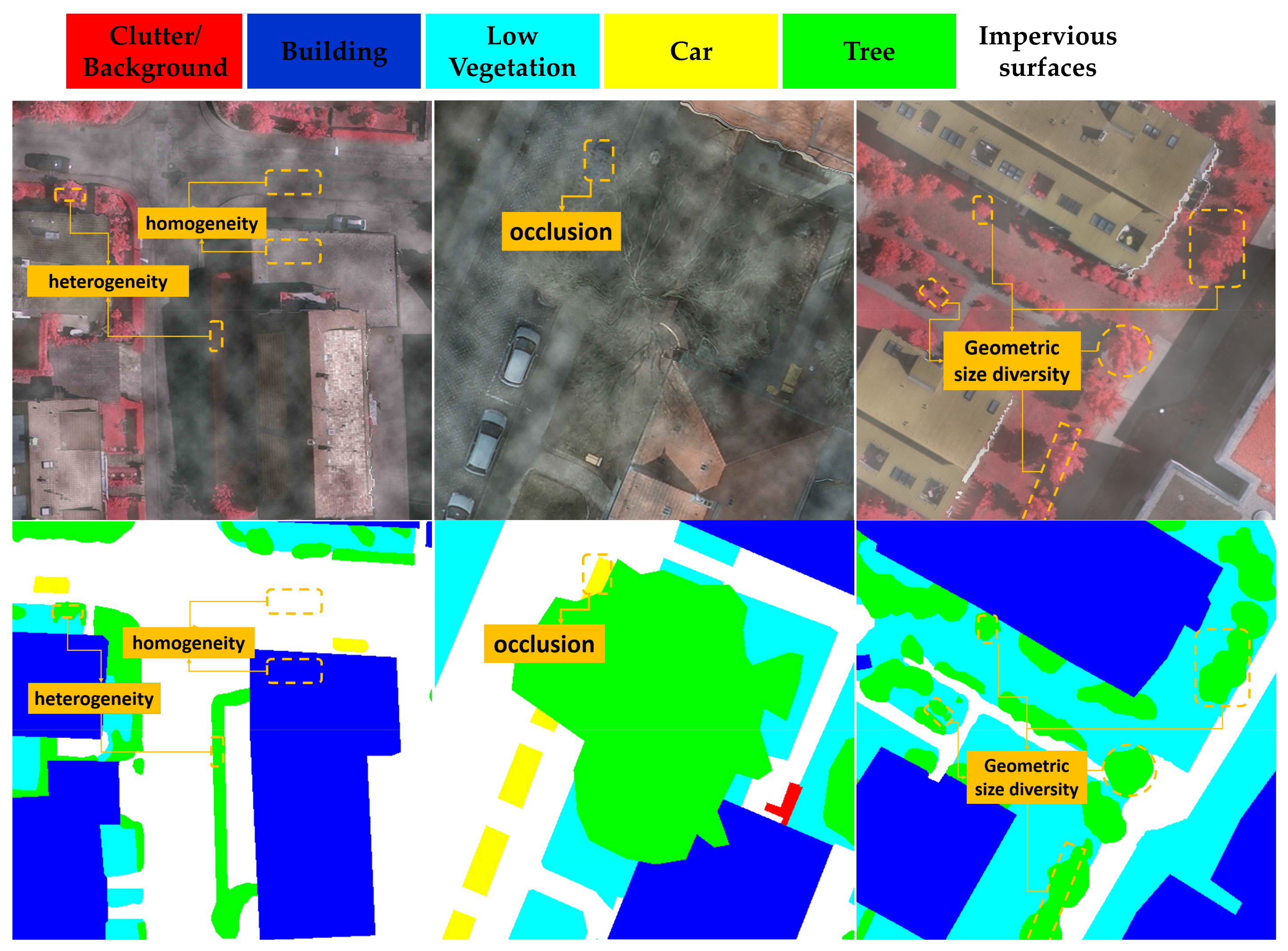
Figure 1.
Challenges associated with robust LCC in the areas covered with fog. The first row is the fog corrupted image and the second row is the corresponding ground truth (GT).
Figure 1.
Challenges associated with robust LCC in the areas covered with fog. The first row is the fog corrupted image and the second row is the corresponding ground truth (GT).
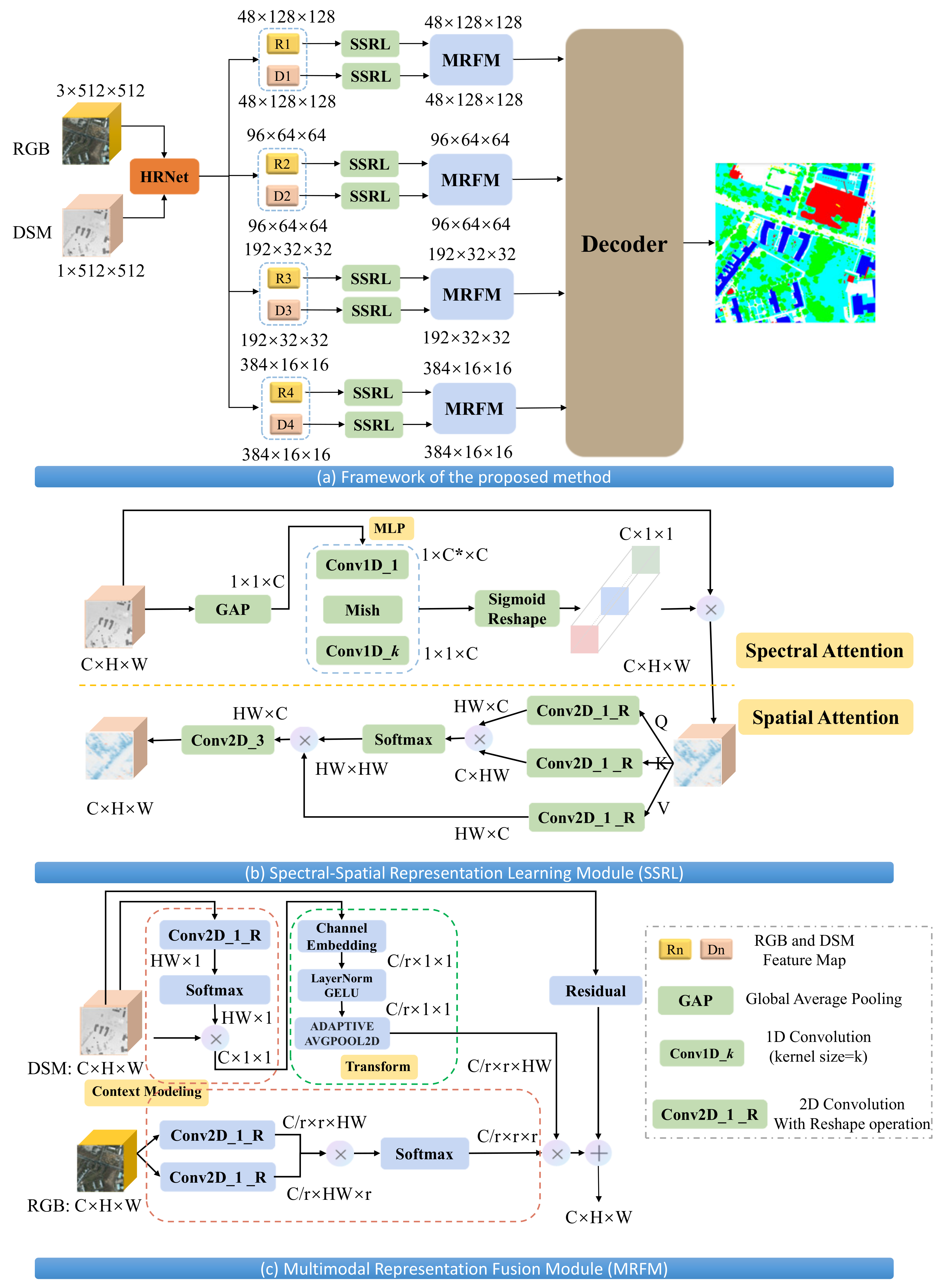
Figure 2.
(a) Illustration of the proposed framework for LCC in foggy conditions. The input consists of a pair of the optical image and DSM. UperHead is selected as the decoder. (b) Detailed design of SSRL, which is composed of Spectral Attention and Spatial Attention modules. and are different channel numbers. (c) The framework of MRFM is to explore the complementarity of heterogeneous inputs.
Figure 3.
Overview of the backbone HRNet. HRNet maintains high-resolution representations and exchanges information throughout branches by means of and convolution. It can cope well with intra-class heterogeneity and multi-scale issues in RSIs with fog.
Figure 3.
Overview of the backbone HRNet. HRNet maintains high-resolution representations and exchanges information throughout branches by means of and convolution. It can cope well with intra-class heterogeneity and multi-scale issues in RSIs with fog.
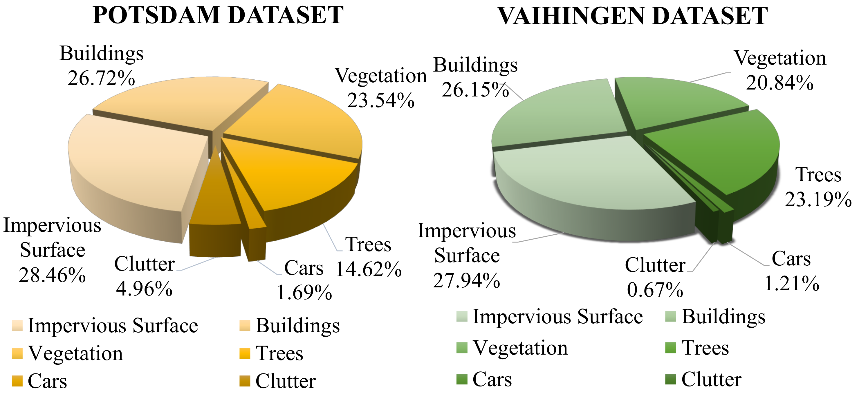
Figure 4.
Illustrations about the composition of each class in ISPRS datasets.
Figure 4.
Illustrations about the composition of each class in ISPRS datasets.
Figure 5.
Illustrations about samples of Potsdam and Vaihingen dataset. Augmented means the image after the augmentation operation.
Figure 5.
Illustrations about samples of Potsdam and Vaihingen dataset. Augmented means the image after the augmentation operation.
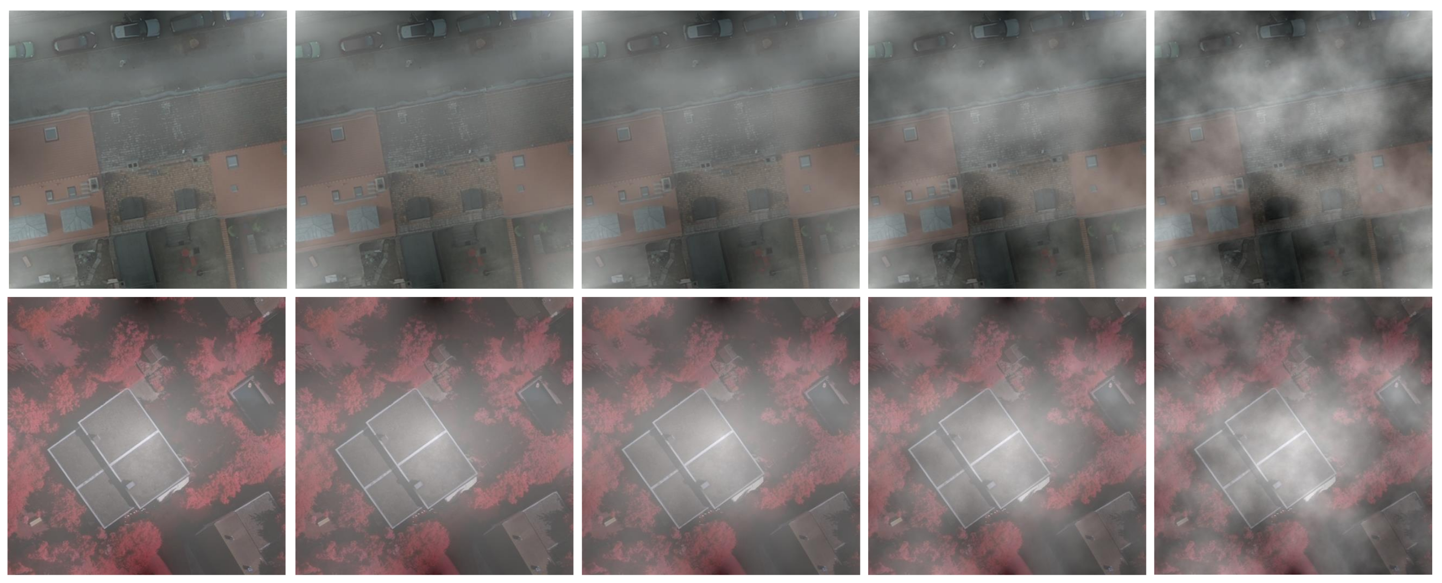
Figure 6.
Illustrations of five severity levels of fog rendered the ISPRS dataset. First row: Potsdam. Second row: Vaihingen.
Figure 6.
Illustrations of five severity levels of fog rendered the ISPRS dataset. First row: Potsdam. Second row: Vaihingen.
Figure 7.
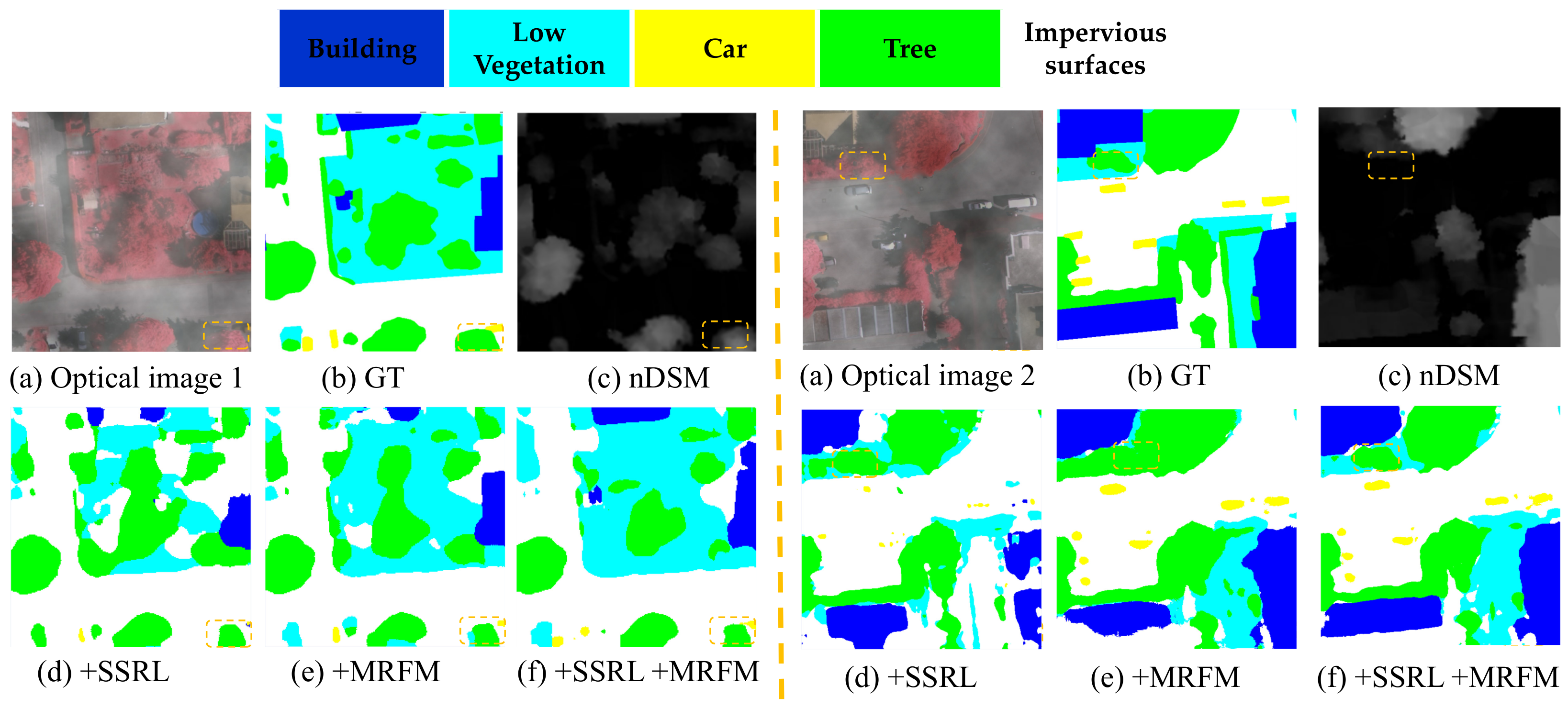
Illustrations about some ablation results of each component in the framework. In this case, optical images are corrupted by fog, which belongs to severity level 2.
Figure 7.
Illustrations about some ablation results of each component in the framework. In this case, optical images are corrupted by fog, which belongs to severity level 2.
Figure 8.
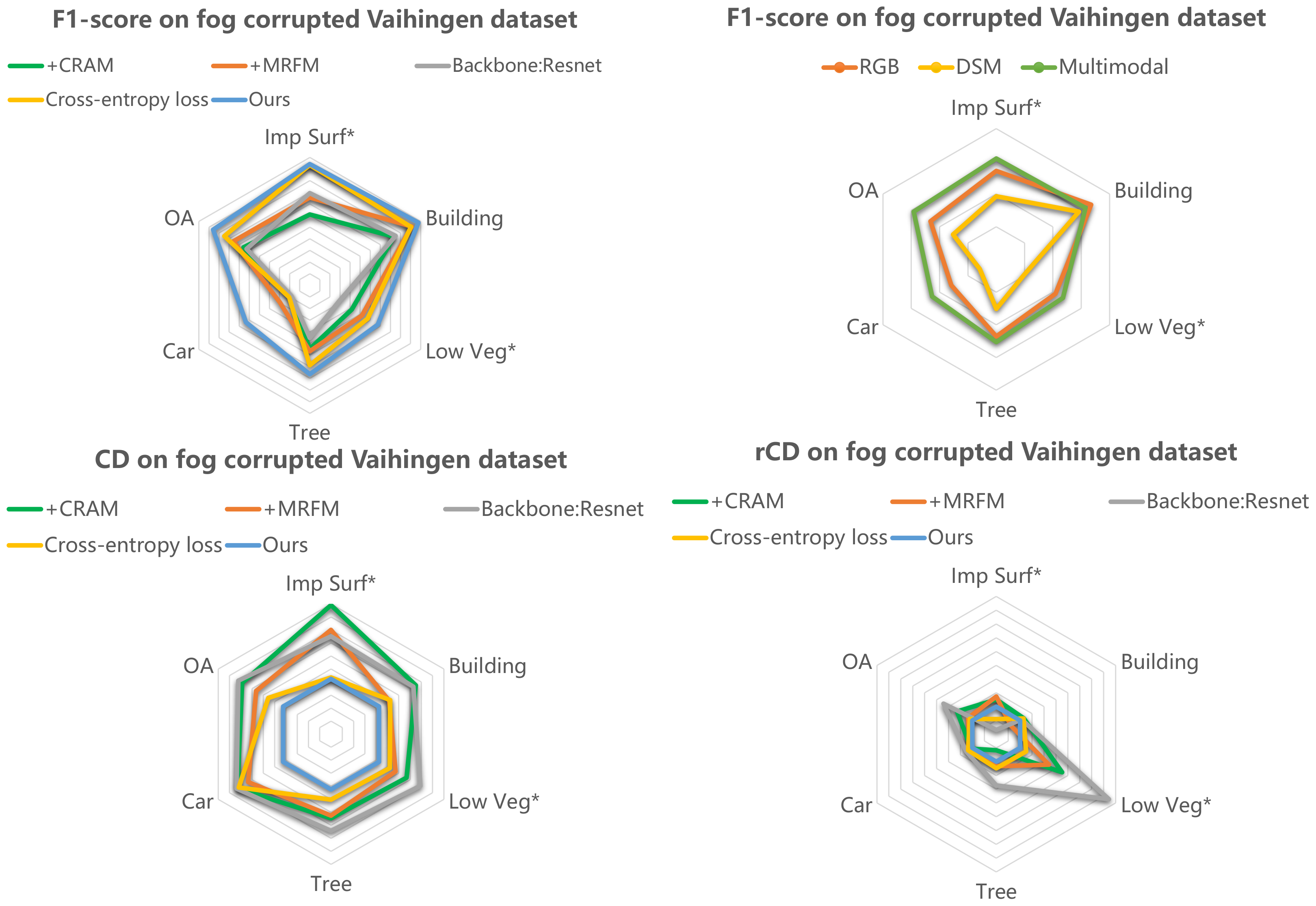
Radar plot visualization of the ablation study results. The first in top two is the classification result when different modules are integrated into the backbone. The second is about different inputs. Based on the radar plots regarding and , the smaller envelope range is indicative of a model that is more robust on a fog-corrupted test set.
Figure 9.
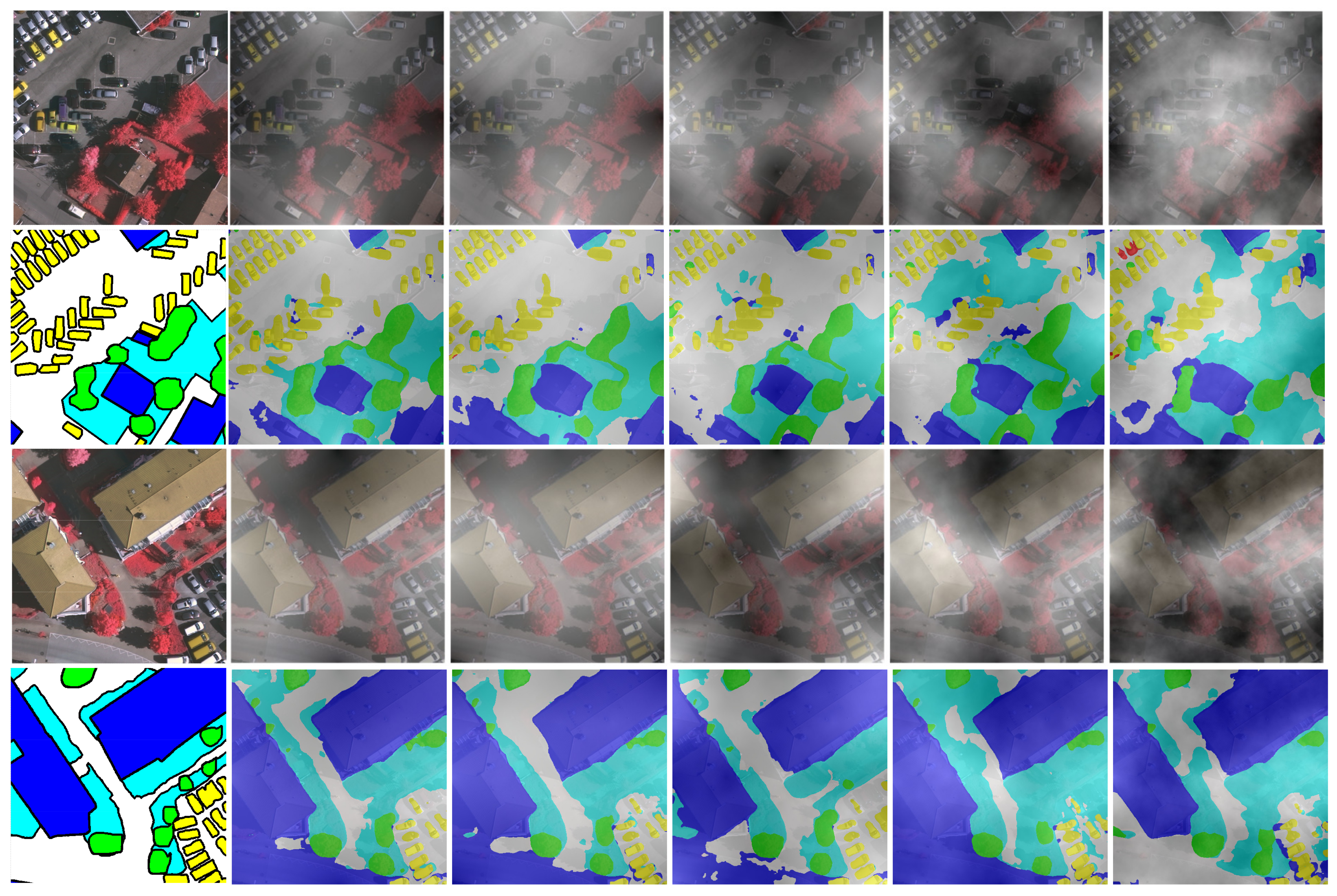
Comparing the LCC results across different corruption levels. 1st column displays the clean image and ground truth. Others are images with fog of various severity levels, accompanied by the corresponding semantic labeling result. From left to right, the fog intensity increases gradually.
Figure 9.
Comparing the LCC results across different corruption levels. 1st column displays the clean image and ground truth. Others are images with fog of various severity levels, accompanied by the corresponding semantic labeling result. From left to right, the fog intensity increases gradually.
Figure 10.
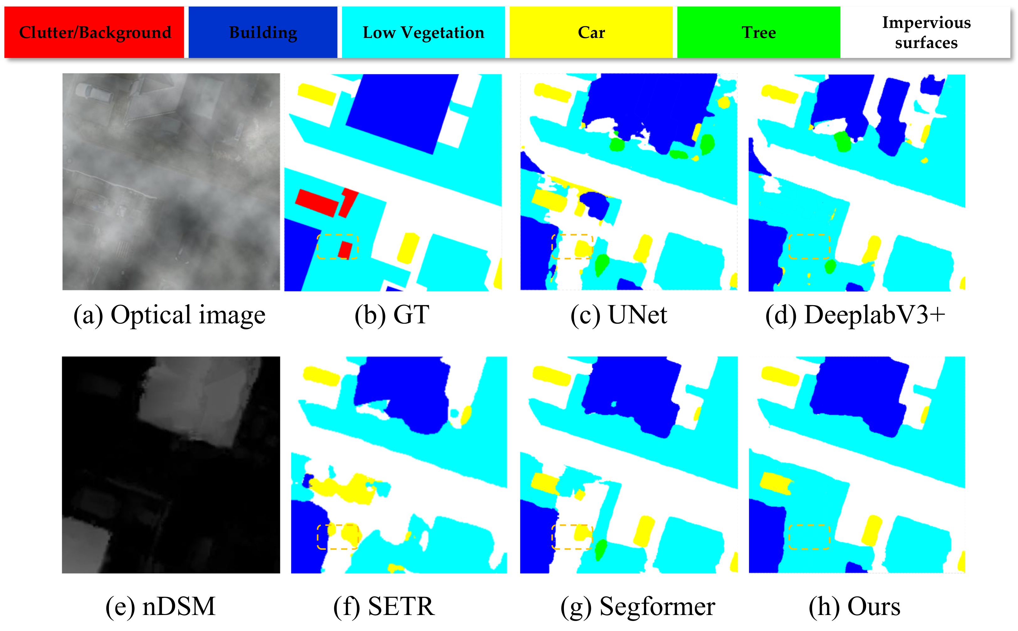
Qualitative comparisons between different methods applied to semantic segmentation of RSIs. The optical image is corrupted by the third severity level of fog.
Figure 10.
Qualitative comparisons between different methods applied to semantic segmentation of RSIs. The optical image is corrupted by the third severity level of fog.
Figure 11.
Qualitative comparisons between different methods applied to semantic segmentation of RSIs. The optical image is corrupted by the fourth severity level of fog.
Figure 11.
Qualitative comparisons between different methods applied to semantic segmentation of RSIs. The optical image is corrupted by the fourth severity level of fog.
Figure 12.
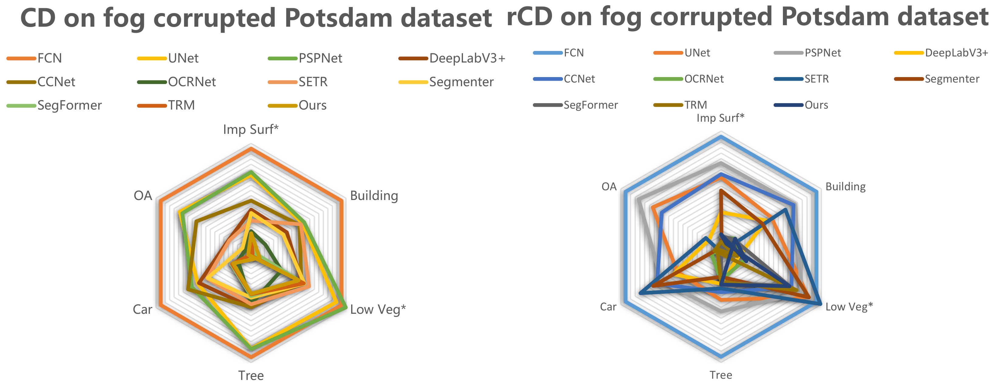
Radar plot for the robust performance of several SOTAs on the Potsdam test set. The envelope area of a robust model should be small and balanced. Although ViTs can boost the performance, CNNs manifest stronger robustness compared with ViTs.
Figure 12.
Radar plot for the robust performance of several SOTAs on the Potsdam test set. The envelope area of a robust model should be small and balanced. Although ViTs can boost the performance, CNNs manifest stronger robustness compared with ViTs.
Table 1.
Detailed HRNET specifications about every stage and channels.
Table 1.
Detailed HRNET specifications about every stage and channels.
| Downsp. Rate | Stage1 | Stage2 | Stage3 | Stage4 |
|---|
| 4× | | | | |
| 8× | | | | |
| 16 × | | | | |
| 32 × | | | | |
Table 2.
Ablation study results with different components integrated based on the clean and fog corrupted variants of the Vaihingen test set. The is averaged across five severity levels. The best results are marked in bold.
Table 2.
Ablation study results with different components integrated based on the clean and fog corrupted variants of the Vaihingen test set. The is averaged across five severity levels. The best results are marked in bold.
| Method | Per-Class (%) | Mean F1 (%) | OA (%) |
|---|
| Imp Surf* | Building | Low Veg* | Tree | Car |
|---|
| Baseline | SSRL | MRFM | Loss | Clean | Fog | Clean | Fog | Clean | Fog | Clean | Fog | Clean | Fog | Clean | Fog | Clean | Fog |
| H | ✓ | | U | 84.93 | 72.18 | 88.71 | 76.71 | 81.70 | 68.32 | 82.51 | 70.93 | 83.46 | 63.82 | 84.26 | 70.39 | 85.92 | 73.12 |
| H | | ✓ | U | 88.13 | 75.10 | 90.97 | 80.21 | 82.66 | 70.38 | 84.36 | 71.32 | 85.79 | 65.92 | 86.38 | 72.58 | 86.91 | 75.16 |
| R | ✓ | ✓ | U | 85.94 | 75.86 | 88.85 | 77.04 | 82.96 | 65.71 | 83.83 | 69.01 | 84.09 | 63.65 | 85.13 | 70.25 | 86.63 | 72.53 |
| H | ✓ | ✓ | C | 91.74 | 80.70 | 92.05 | 80.08 | 81.86 | 71.47 | 86.97 | 73.74 | 84.21 | 64.08 | 87.36 | 74.01 | 88.55 | 76.97 |
| H | ✓ | ✓ | U | 92.98 | 80.85 | 93.19 | 81.54 | 83.39 | 73.50 | 87.91 | 75.28 | 92.12 | 72.67 | 89.92 | 76.77 | 90.49 | 79.15 |
Table 3.
in ablation study with different components integrated based on clean and fog corrupted variants of the Vaihingen test set. Our framework is regarded as the reference and values above 100% denote a decrease in robustness compared with the reference. The highest is bold.
Table 3.
in ablation study with different components integrated based on clean and fog corrupted variants of the Vaihingen test set. Our framework is regarded as the reference and values above 100% denote a decrease in robustness compared with the reference. The highest is bold.
| Method | for Per-Class (%) | Mean (%) | for OA (%) |
|---|
| Imp Surf* | Building | Low Veg* | Tree | Car |
|---|
| Baseline | SSRL | MRFM | Loss | Clean | Fog | Clean | Fog | Clean | Fog | Clean | Fog | Clean | Fog | Clean | Fog | Clean | Fog |
| H | ✓ | | U | 214.50 | 145.23 | 165.73 | 126.15 | 110.16 | 119.53 | 144.69 | 117.61 | 209.78 | 132.41 | 156.06 | 127.44 | 148.08 | 128.94 |
| H | | ✓ | U | 169.01 | 130.01 | 132.58 | 107.19 | 104.39 | 111.78 | 129.40 | 116.04 | 180.21 | 124.74 | 135.05 | 118.01 | 137.69 | 119.14 |
| R | ✓ | ✓ | U | 200.23 | 126.05 | 163.72 | 124.36 | 102.58 | 129.40 | 133.78 | 125.37 | 201.80 | 133.03 | 147.44 | 128.04 | 140.65 | 131.75 |
| H | ✓ | ✓ | C | 117.66 | 100.77 | 116.64 | 107.90 | 109.22 | 107.66 | 107.81 | 106.24 | 200.27 | 131.45 | 125.30 | 111.86 | 120.36 | 110.48 |
| H | ✓ | ✓ | U | 100.00 | 100.00 | 100.00 | 100.00 | 100.00 | 100.00 | 100.00 | 100.00 | 100.00 | 100.00 | 100.00 | 100.00 | 100.00 | 100.00 |
Table 4.
The relative in ablation study with different components integrated based on clean and fog corrupted variants of the Vaihingen test set. Lower suggests an improvement of robustness in the presence of fog corruption. The highest is bold.
Table 4.
The relative in ablation study with different components integrated based on clean and fog corrupted variants of the Vaihingen test set. Lower suggests an improvement of robustness in the presence of fog corruption. The highest is bold.
| Method | for Per-Class (%) | Mean (%) | for OA (%) |
|---|
| Baseline | SSRL | MRFM | Loss | Imp Surf* | Building | Low Veg* | Tree | Car |
|---|
| H | ✓ | | U | 105.12 | 103.01 | 135.26 | 91.70 | 101.03 | 105.49 | 112.89 |
| H | | ✓ | U | 107.42 | 92.35 | 124.19 | 103.25 | 102.24 | 104.94 | 103.59 |
| R | ✓ | ✓ | U | 83.10 | 101.36 | 174.43 | 117.31 | 105.13 | 113.17 | 124.28 |
| H | ✓ | ✓ | C | 90.99 | 102.78 | 105.05 | 104.74 | 103.54 | 101.55 | 102.19 |
| H | ✓ | ✓ | U | 100.00 | 100.00 | 100.00 | 100.00 | 100.00 | 100.00 | 100.00 |
Table 5.
Quantitative evaluation for clean and fog corrupted variants of the Vaihingen test set about using different input data. Every is averaged over all five severity levels. The best results are marked in bold.
Table 5.
Quantitative evaluation for clean and fog corrupted variants of the Vaihingen test set about using different input data. Every is averaged over all five severity levels. The best results are marked in bold.
| Method | Per-Class (%) | Mean F1 (%) | OA (%) |
|---|
| Optical | DSM | Imp Surf* | Building | Low Veg* | Tree | Car |
|---|
| Clean | Fog | Clean | Fog | Clean | Fog | Clean | Fog | Clean | Fog | Clean | Fog | Clean | Fog |
|---|
| ✓ | | 90.70 | 77.05 | 91.58 | 83.49 | 82.32 | 70.91 | 85.32 | 73.56 | 90.63 | 65.87 | 88.11 | 74.17 | 88.69 | 73.25 |
| | ✓ | 85.50 | 69.28 | 88.66 | 79.17 | 76.21 | 59.70 | 83.59 | 65.12 | 83.89 | 55.85 | 83.57 | 65.82 | 80.18 | 65.21 |
| ✓ | ✓ | 92.98 | 80.85 | 93.19 | 81.54 | 83.39 | 73.50 | 87.91 | 75.28 | 92.12 | 72.67 | 89.92 | 76.77 | 90.49 | 79.15 |
Table 6.
Quantitative evaluation of on clean and fog corrupted variants of the Vaihingen test set about using different input data. Our framework is regarded as the reference and values above 100% denote a decrease in robustness compared with the reference. The highest is bold.
Table 6.
Quantitative evaluation of on clean and fog corrupted variants of the Vaihingen test set about using different input data. Our framework is regarded as the reference and values above 100% denote a decrease in robustness compared with the reference. The highest is bold.
| Method | for Per-Class (%) | Mean (%) | for OA (%) |
|---|
| Optical | DSM | Imp Surf* | Building | Low Veg* | Tree | Car |
|---|
| Clean | Fog | Clean | Fog | Clean | Fog | Clean | Fog | Clean | Fog | Clean | Fog | Clean | Fog |
|---|
| ✓ | | 132.42 | 119.84 | 123.59 | 89.42 | 106.41 | 109.76 | 121.47 | 106.96 | 118.83 | 124.91 | 117.91 | 111.16 | 118.93 | 128.32 |
| | ✓ | 206.37 | 160.39 | 166.46 | 112.84 | 143.21 | 152.07 | 135.73 | 141.11 | 204.35 | 161.56 | 162.92 | 147.11 | 208.43 | 166.88 |
| ✓ | ✓ | 100.00 | 100.00 | 100.00 | 100.00 | 100.00 | 100.00 | 100.00 | 100.00 | 100.00 | 100.00 | 100.00 | 100.00 | 100.00 | 100.00 |
Table 7.
Quantitative evaluation of on clean and fog corrupted variants of the Vaihingen test set in ablation study about using different input data evaluated. Our framework is regarded as the reference and lower indicates an improvement of robustness in the presence of fog corruption. The highest is bold.
| Method | for Per-Class (%) | Mean (%) | for OA (%) |
|---|
| Optical | DSM | Imp Surf* | Building | Low Veg* | Tree | Car |
|---|
| ✓ | | 112.56 | 69.44 | 115.40 | 93.08 | 127.37 | 105.98 | 136.18 |
| | ✓ | 133.76 | 81.49 | 166.94 | 146.25 | 144.21 | 134.98 | 132.04 |
| ✓ | ✓ | 100.00 | 100.00 | 100.00 | 100.00 | 100.00 | 100.00 | 100.00 |
Table 8.
Quantitative comparison with SOTA methods on the clean and fog corrupted variants of the Potsdam test set. Each is averaged over all severity levels. The best results are marked in bold.
Table 8.
Quantitative comparison with SOTA methods on the clean and fog corrupted variants of the Potsdam test set. Each is averaged over all severity levels. The best results are marked in bold.
| Method | Per-Class (%) | Mean F1 (%) | OA (%) |
|---|
| Imp Surf* | Building | Low Veg* | Tree | Car |
|---|
| Clean | Fog | Clean | Fog | Clean | Fog | Clean | Fog | Clean | Fog | Clean | Fog | Clean | Fog |
|---|
| FCN [5] | 85.15 | 63.22 | 86.08 | 67.12 | 79.02 | 63.15 | 81.72 | 63.58 | 78.24 | 55.61 | 82.04 | 62.54 | 85.86 | 58.33 |
| UNet [6] | 85.61 | 66.93 | 88.17 | 72.79 | 79.31 | 63.99 | 79.16 | 64.77 | 80.61 | 62.89 | 82.57 | 66.27 | 86.25 | 61.85 |
| PSPNet [12] | 86.34 | 66.52 | 89.79 | 72.55 | 77.34 | 62.46 | 79.88 | 64.73 | 80.95 | 61.74 | 82.86 | 65.60 | 88.34 | 62.31 |
| DeepLabV3+[13] | 87.73 | 71.83 | 90.06 | 75.08 | 80.27 | 69.59 | 83.89 | 70.56 | 81.23 | 63.12 | 84.64 | 70.04 | 88.76 | 70.86 |
| CCNet [43] | 89.49 | 70.55 | 90.37 | 73.24 | 83.91 | 69.71 | 84.47 | 70.59 | 80.63 | 60.98 | 85.77 | 69.01 | 88.27 | 64.91 |
| OCRNet [44] | 88.77 | 74.86 | 90.69 | 78.19 | 84.02 | 72.95 | 84.11 | 71.02 | 85.33 | 70.79 | 86.58 | 73.56 | 89.31 | 74.92 |
| SETR [27] | 86.09 | 73.38 | 89.53 | 73.04 | 84.57 | 68.44 | 84.61 | 70.98 | 85.93 | 64.71 | 86.15 | 70.11 | 89.26 | 70.99 |
| Segmenter [45] | 89.94 | 72.30 | 90.22 | 75.61 | 84.58 | 69.21 | 84.77 | 71.90 | 84.85 | 64.83 | 86.87 | 70.77 | 89.88 | 73.42 |
| SegFormer [28] | 89.53 | 75.52 | 92.40 | 80.02 | 84.07 | 69.99 | 85.38 | 72.13 | 83.05 | 69.48 | 86.89 | 73.43 | 90.01 | 74.91 |
| TRM [15] | 89.11 | 75.57 | 91.45 | 80.61 | 83.83 | 69.29 | 85.56 | 72.37 | 83.58 | 69.62 | 86.71 | 73.49 | 89.92 | 75.27 |
| Ours | 89.31 | 75.16 | 92.49 | 80.70 | 84.23 | 70.15 | 85.83 | 72.45 | 82.08 | 69.83 | 86.79 | 73.66 | 90.17 | 76.57 |
Table 9.
Quantitative evaluation of on clean and fog corrupted variants of Potsdam test set about different SOTA methods. FCN is regarded as the reference and values lower than 100% represent an improvement in the robust performance compared with the reference. The minimum in each column is bold.
Table 9.
Quantitative evaluation of on clean and fog corrupted variants of Potsdam test set about different SOTA methods. FCN is regarded as the reference and values lower than 100% represent an improvement in the robust performance compared with the reference. The minimum in each column is bold.
| Method | for Per-Class (%) | for Mean F1 (%) | for OA (%) |
|---|
| Imp Surf* | Building | Low Veg* | Tree | Car |
|---|
| Clean | Fog | Clean | Fog | Clean | Fog | Clean | Fog | Clean | Fog | Clean | Fog | Clean | Fog |
|---|
| FCN [5] | 100.00 | 100.00 | 100.00 | 100.00 | 100.00 | 100.00 | 100.00 | 100.00 | 100.00 | 100.00 | 100.00 | 100.00 | 100.00 | 100.00 |
| UNet [6] | 96.90 | 89.91 | 84.99 | 82.76 | 98.62 | 97.72 | 114.00 | 96.73 | 89.11 | 83.60 | 97.05 | 90.02 | 97.24 | 91.55 |
| PSPNet [12] | 91.99 | 91.03 | 73.35 | 83.49 | 108.01 | 101.87 | 110.07 | 96.84 | 87.55 | 86.19 | 95.44 | 91.82 | 82.46 | 90.45 |
| DeepLabV3+[13] | 82.63 | 76.59 | 71.41 | 75.79 | 94.04 | 82.52 | 88.13 | 80.83 | 86.26 | 83.08 | 85.56 | 79.98 | 79.49 | 69.93 |
| CCNet [43] | 70.77 | 80.07 | 69.18 | 81.39 | 76.69 | 82.20 | 84.96 | 80.75 | 89.02 | 87.90 | 79.22 | 82.71 | 82.96 | 84.21 |
| OCRNet [44] | 75.62 | 68.35 | 66.88 | 66.33 | 76.17 | 73.41 | 86.93 | 79.57 | 67.42 | 65.80 | 74.71 | 70.57 | 75.60 | 60.19 |
| SETR [27] | 93.67 | 72.38 | 75.22 | 82.00 | 73.55 | 85.64 | 84.19 | 79.68 | 64.66 | 79.50 | 77.15 | 79.78 | 75.95 | 69.62 |
| Segmenter [45] | 67.74 | 75.31 | 70.26 | 74.18 | 73.50 | 83.55 | 83.32 | 77.16 | 69.62 | 79.23 | 73.10 | 78.02 | 71.57 | 63.79 |
| SegFormer [28] | 70.51 | 66.56 | 54.60 | 60.77 | 75.93 | 81.44 | 79.98 | 76.52 | 77.90 | 68.75 | 73.03 | 70.93 | 70.65 | 60.21 |
| TRM [15] | 73.33 | 66.42 | 61.42 | 58.97 | 77.07 | 83.34 | 78.99 | 75.86 | 75.46 | 68.44 | 74.03 | 70.76 | 71.29 | 59.35 |
| Ours | 71.99 | 67.54 | 53.95 | 58.70 | 75.17 | 81.00 | 77.52 | 75.65 | 82.35 | 67.97 | 73.57 | 70.31 | 69.52 | 56.23 |
Table 10.
Quantitative evaluation of on clean and fog corrupted variants of Potsdam test set about different SOTA methods. FCN is regarded as the reference and values lower than 100% represent an improvement in the robust performance compared to the reference. The minimum in each column is in bold.
Table 10.
Quantitative evaluation of on clean and fog corrupted variants of Potsdam test set about different SOTA methods. FCN is regarded as the reference and values lower than 100% represent an improvement in the robust performance compared to the reference. The minimum in each column is in bold.
| Method | for Per-Class (%) | Mean (%) | for OA (%) |
|---|
| Imp Surf* | Building | Low Veg* | Tree | Car |
|---|
| FCN [5] | 100.00 | 100.00 | 100.00 | 100.00 | 100.00 | 100.00 | 100.00 |
| UNet [6] | 85.18 | 81.12 | 96.53 | 79.33 | 78.30 | 83.55 | 88.63 |
| PSPNet [12] | 90.38 | 90.93 | 93.76 | 83.52 | 84.89 | 88.49 | 94.55 |
| DeepLabV3+ [13] | 72.50 | 79.01 | 67.30 | 73.48 | 80.03 | 74.85 | 65.02 |
| CCNet [43] | 86.37 | 90.35 | 89.48 | 76.52 | 86.83 | 85.92 | 84.85 |
| OCRNet [44] | 63.43 | 65.93 | 69.75 | 72.16 | 64.25 | 66.76 | 52.27 |
| SETR [27] | 57.96 | 86.97 | 101.64 | 75.14 | 93.77 | 82.21 | 66.36 |
| Segmenter [45] | 80.44 | 77.06 | 96.85 | 70.95 | 88.47 | 82.55 | 59.79 |
| SegFormer [28] | 63.89 | 65.30 | 88.72 | 73.04 | 59.96 | 68.99 | 54.85 |
| TRM [15] | 61.74 | 57.17 | 91.62 | 72.71 | 61.69 | 67.74 | 53.21 |
| Ours | 64.52 | 62.18 | 88.72 | 73.76 | 54.13 | 67.31 | 49.40 |
