Abstract
In this paper, we obtain the intensity and phase distributions of the scattering and external fields of a vector Bessel–Gaussian vortex beam in the far-field region after being scattered by a particle. In our analysis, we use the Generalized Lorenz–Mie theory (GLMT) and the angular spectrum decomposition method (ASDM). The orbital angular momentum (OAM) spectra of the fields are analyzed by using the spiral spectrum expansion method, which is a frequently used tool for studying the propagation of vortex beams in turbulent atmospheres. Both scattered and external fields show a significant difference in spiral spectra for particles with different characteristic parameters, such as the size and complex refractive index. We also examine sampling the phase along with a circle and show that it is unable to fully express the information of the fields. This study can provide a theoretical basis for the inversion of characteristic parameters of the Bessel–Gaussian vortex beam and spherical particle by OAM spectra with applications in remote sensing engineering.
1. Introduction
Since the 1990s, when the concept of orbital angular momentum (OAM) was proposed by Allen [1], structured beams carrying OAM have been widely used in optical fields. Instances are optical manipulation [2], imaging [3], and optical communication [4,5]. Furthermore, in the particular case of a MIMO system, beams with different OAM modes can potentially increase the capacity of radio communication systems under certain particular conditions [6,7]. Therefore, there have been many studies on the application of vortex beams in antenna design [8,9], radar imaging [10] and target detection [11]. It was shown that the transmission performance of vortex beams is better than that of plane waves [12] and the information carried by vortex beams is more easily obtained by the receiver [13]. This is mainly due to the scattering and transmission characteristics of typical vortex beams.
Techniques based on optics are often used for detecting the physical and chemical properties of substances [14]. The spiral spectrum of the reflected or transmitted field of the vortex beam obtained at the receiving end can be also used for inferring and inversing the information of the transmission channel or target.
Most of the current research on the spiral spectrum characteristics of the OAM beams are focused on the macro transmission channels, such as turbulent atmosphere [15,16,17,18,19,20] and underwater environment [21,22,23,24,25], which are related to the modelling of random media. There are, however, few studies on the scattering characteristics and OAM spectrum of vortex beams irradiating a specific target. In 2012, D. Petrov et al. [26] obtained the spiral spectra scattered off a transparent sphere illuminated by a Laguerre–Gaussian beam. They showed that the geometric properties of the sphere, e.g., the position, can be determined based on the scattering spiral spectrum data. Furthermore, the intensity distribution and OAM mode distortion of a Laguerre–Gaussian vortex beam reflected and transmitted by a non-uniform plasma plate were also examined by Li [27]. Later in 2020, Liu [28] used the physical optical algorithm to investigate the backscattering characteristics of an ideal conductive sphere and a PEC cone illuminated by a vortex beam. They then used phase sampling along the circumference of the scattered field profile and concluded that the scattering field of a symmetric object remains a vortex field, and the topological charge is the same as that of the incident field.
Using the spiral spectrum expansion method, some of the above works take samples along the circumference of the field profile, whereas others sample the whole profile. In this paper, we investigate these two sampling approaches and compare their computational differences and their pros and cons.
Amongst many existing types of vortex beams, the high-order Bessel beam is often used. This is due to the properties, including non-diffraction [29,30] and self-healing [31,32]. The energy of a high-order Bessel beam is, however, infinite in radial distribution [33], hence unattainable in practice. To address this issue, instead of the high-order Bessel beam, an approximated non-diffraction beam, namely, the high-order Bessel–Gaussian beam, is used. Characteristics of the Bessel–Gaussian vortex beams, including transmission in turbulent media [34,35,36], self-healing [37,38], and tight focusing [39] are discussed. Nevertheless, to the best of our knowledge, the interactions between vector high-order Bessel–Gaussian beams and small particles have not been investigated. In our previous works, we derived the beam shape coefficients of polarized Bessel–Gaussian vortex beams [40]. Further, in [41], we studied the scattering of vector Bessel–Gaussian vortex beams caused by spherical particles with non-uniform structure and electric charges. In this paper, we further investigate transmission information of the vector Bessel–Gaussian vortex beam and explore a wider range of potential applications.
This paper is organized as follows: Section 2 presents the theoretical method, derivations of the field distribution, and the OAM spectrum calculations. In Section 3, we then investigate how the changes in characteristic parameters of the particle and the beam affect the OAM spectrum, where three polarization states are considered. The paper is then concluded in Section 4. The appendix shows the beam shape coefficients of differently polarized incident beams.
2. Theoretical Background
2.1. GLMT of a Sphere Illuminated by an Arbitrarily Shaped Beam
According to the Generalized Lorenz–Mie theory, the incident and scattered fields of a spherical particle irradiated by a shaped beam can be expressed by the vector spherical wave functions (, ) multiplied by the beam shape coefficients (, ) [42,43]:
where k = 2π/λ is the wavenumber and
and in Equations (3) and (4) are the expansion coefficients of the scattered field defined as:
and are Mie scattering coefficients and can be derived based on the boundary conditions. The boundary conditions for a uniform and isotropic dielectric sphere, and a charged sphere were obtained in [44], and [45], respectively. Therefore, the specific expressions of their Mie scattering coefficients were derived.
For a homogeneous and isotropic dielectric sphere, the Mie scattering coefficients are
and for a charged sphere,
where m is the complex refractive index of the sphere relative to the surrounding vacuum environment. Also, σs is the conductivity of a sphere carrying electric charges [45,46]:
and ωs is the plasma frequency derived by , me and q are the mass and charge of an electron, respectively, i.e., me = 9.109 × 10⁻³¹ kg and q = 1.602 × 10⁻¹⁹ C. is the surface electrostatic potential of a charged sphere, a is the radius of the sphere, and ε0 is the permittivity of the vacuum. Besides, , kB = 1.3807 × 10⁻²³ J/K is the Boltzmann’s constant, T is the temperature of the sphere in Kelvin, ħ denotes the reduced Planck constant, and ħ = 1.05457 × 10⁻³⁴ J s. Given the frequency of the incident beam and the radius of the sphere, the conductivity can be determined by the surface electrostatic potential φ and the temperature T.
As is seen above, given the beam shape coefficients of the vector Bessel–Gaussian vortex beams, the incident field and scattered field in the far region can be obtained using Equations (1)–(4).
The derivation of beam shape coefficients of Bessel–Gaussian vortex beams with different polarization states is presented in Appendix A.
2.2. Spiral Spectrum Expansion Method
Any field distribution can be considered as the superposition of multiple spiral harmonics [47,48,49].
The expansion coefficients are
The energy content or weight of each spiral harmonic of a field can therefore be determined as the following:
The weight, , corresponds to the detection probability on the measurement plane, where the orbital angular momentum is n.
Using the spiral spectrum expansion method, there are two main approaches to analyzing the spiral spectrum characteristics of the field. One approach is to ignore the radial distribution of the field followed by sampling along the circle at a certain radius, see, e.g., [28,50,51,52]. An alternative approach, e.g., [27,47,48,49] is to sample radial and angular distributions of the field on the whole measurement plane at the receiving end.
3. Simulation and Discussion
First, in order to verify the correctness of the algorithm we use, a validation example is used to compare the calculation results of the Mie scattering theory with those of the electromagnetic (EM) simulation software FEKO. Subject to the source of FEKO, a Bessel–Gaussian beam with x-polarization is considered to irradiate a uniform and homogeneous dielectric sphere of complex refractive index and radius a = 0.5 μm. The wavelength of the incident beam is λ = 1.064 μm, the order is l = 0, the conic angle is θb = 0°, and the beam waist radius . The radar cross section (RCS) and the scattered field distribution calculated by the GLMT and FEKO are compared. The measurement plane of the scattered field is located at z = 50 μm, and the results are shown in Figure 1. It is obvious that the results match very well and the relative errors are negligible.
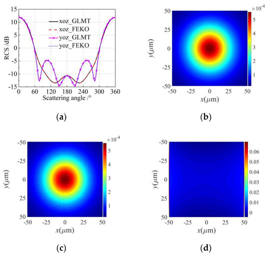
Figure 1.
Comparison of the results calculated by the Mie scattering theory and FEKO: panel (a) is the radar cross section (RCS); panels (b) and (c) are the scattered field distributions obtained by the GLMT algorithm and FEKO simulation, respectively; the relative error between them is shown in panel (d).
In the following simulations of the field sampling, we consider the OAM modes from −5 to 5. We further set the radial, and angular sampling intervals to 0.1 μm, and 1°, respectively.
Considering the y-polarized Bessel–Gaussian beam as an example, the topological charges of the incident beam are 1, 2, 3, and 4, respectively. Unless otherwise specified, here the beam wavelength is 1.064 μm, the conic angle is 25° and the waist radius is 0.5 μm.
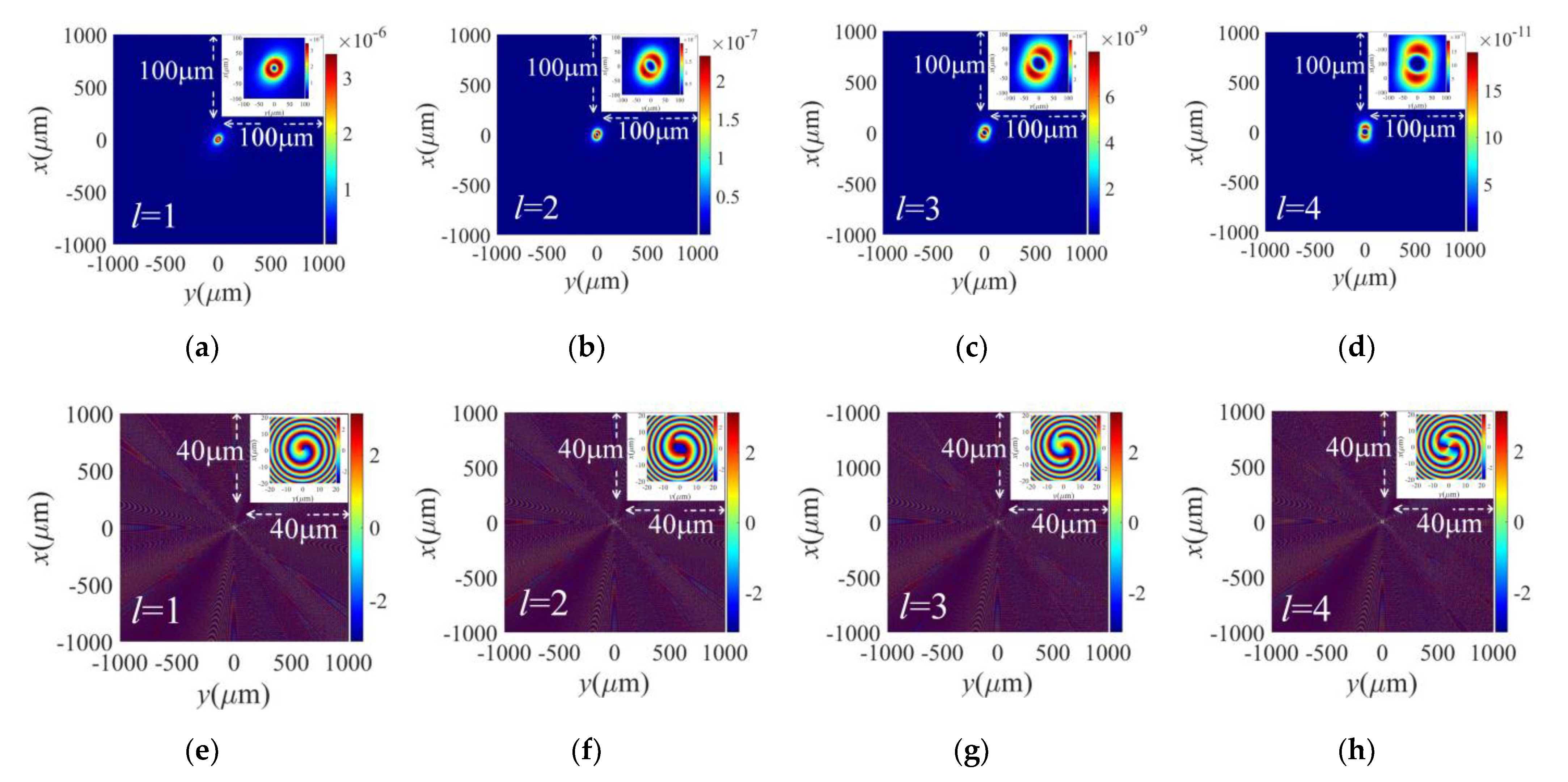
Figure 2 shows the intensity and phase distributions of the y-polarized Bessel–Gaussian vortex beams at the source plane. The topological charges corresponding to the left panels to right are 1–4, respectively. Panels (a)–(d) present intensity and (e)–(h) show phase. The intensity distribution of the incident field of beam presents a hollow structure and the hollow shape is similar to an ellipse. It is not completely uniform and symmetrical in the angular space, but it follows the basic characteristics of the vortex beam. In other words, the greater the topological charge, the weaker the intensity and the larger the hollow size. Note that the panels at the bottom show the phase distributions, where the changes in the wavefront phase reflect the orbital angular momentum mode carried by the incident beam.
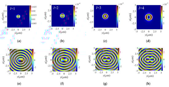
Figure 2.
The intensity and phase distributions of the incident field of y-polarized Bessel–Gaussian beams with different topological charges at the source plane: panels (a–d); and (e–h) show intensity, and phase, respectively. The corresponding topological charge from left to right is 1–4.
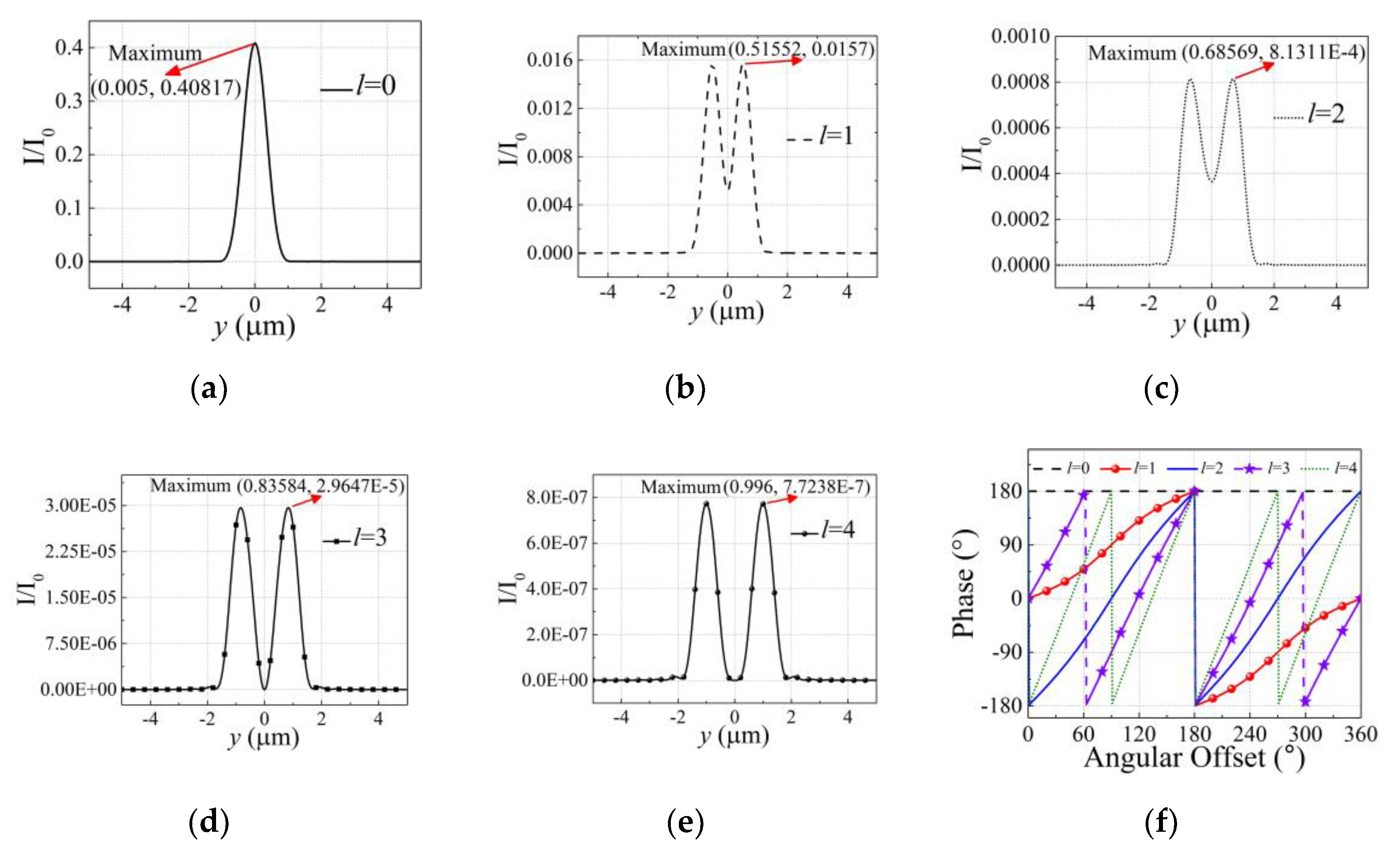
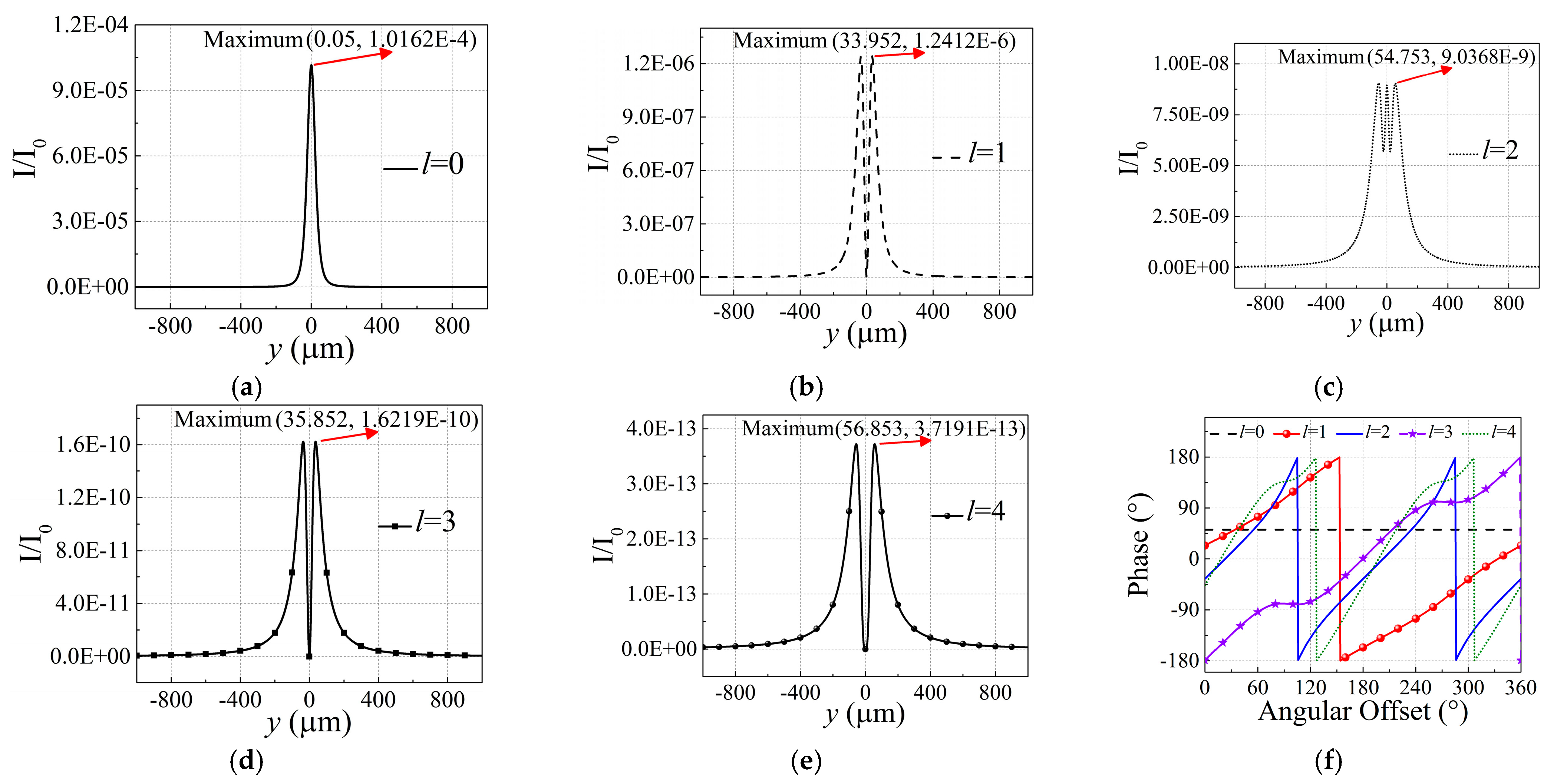
As was seen above, there are two ways to detect the spiral spectrum according to the field distribution including sampling along the circumference at a certain radius and sampling the whole measurement plane. The OAM modes of the incident beam at the source plane are calculated according to these two sampling methods. Figure 3 provides the one-dimensional intensity of the incident field in the polarization direction (i.e., y-direction), and marks the specific coordinates with the maximum intensity. Taking the position as the determined radius, we then conduct phase sampling on the circle. A similar approach based on taking the intensity in the polarization direction as a sample was also considered in [28].

Figure 3.
(a–e) show the one-dimensional intensity distribution of the incident beams with different topological charges in the polarization direction; (f) shows the phase sampling results along the circumference.
Panels (a)–(e) in Figure 3 show the one-dimensional intensity distribution of the incident field in the polarization direction for the topological charges of 0, 1, 2, 3 and 4, respectively. We also marked the specific coordinates with the maximum intensity. It can be seen that for the topological charges of 1 and 2, the central intensity is a valley with a non-zero value. In contrast, for the topological charges of 3 and 4, the intensity in the center is further reduced to 0. The position with the intensity peak indicates the size of the hollow. In Figure 3f we consider the location where the intensity has its maximum value as the radius and plot the phase samples along the circumference. Figure 3f shows that the phase sampling results along the circle can intuitively characterize the topological charge of the incident beam, i.e., through the relationship between the phase change and 2π within the sampling angle range, regardless of whether the phase changes regularly or not.
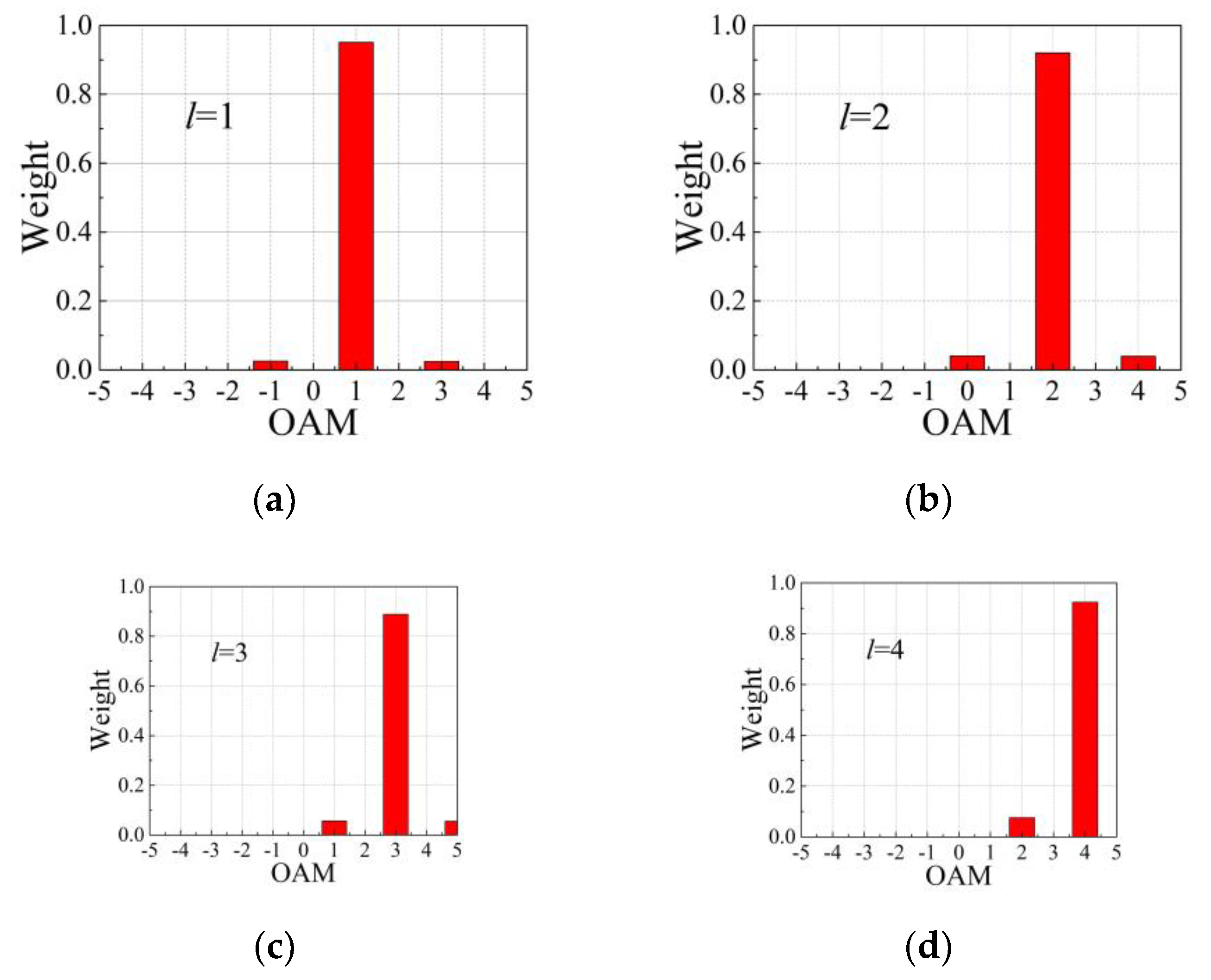
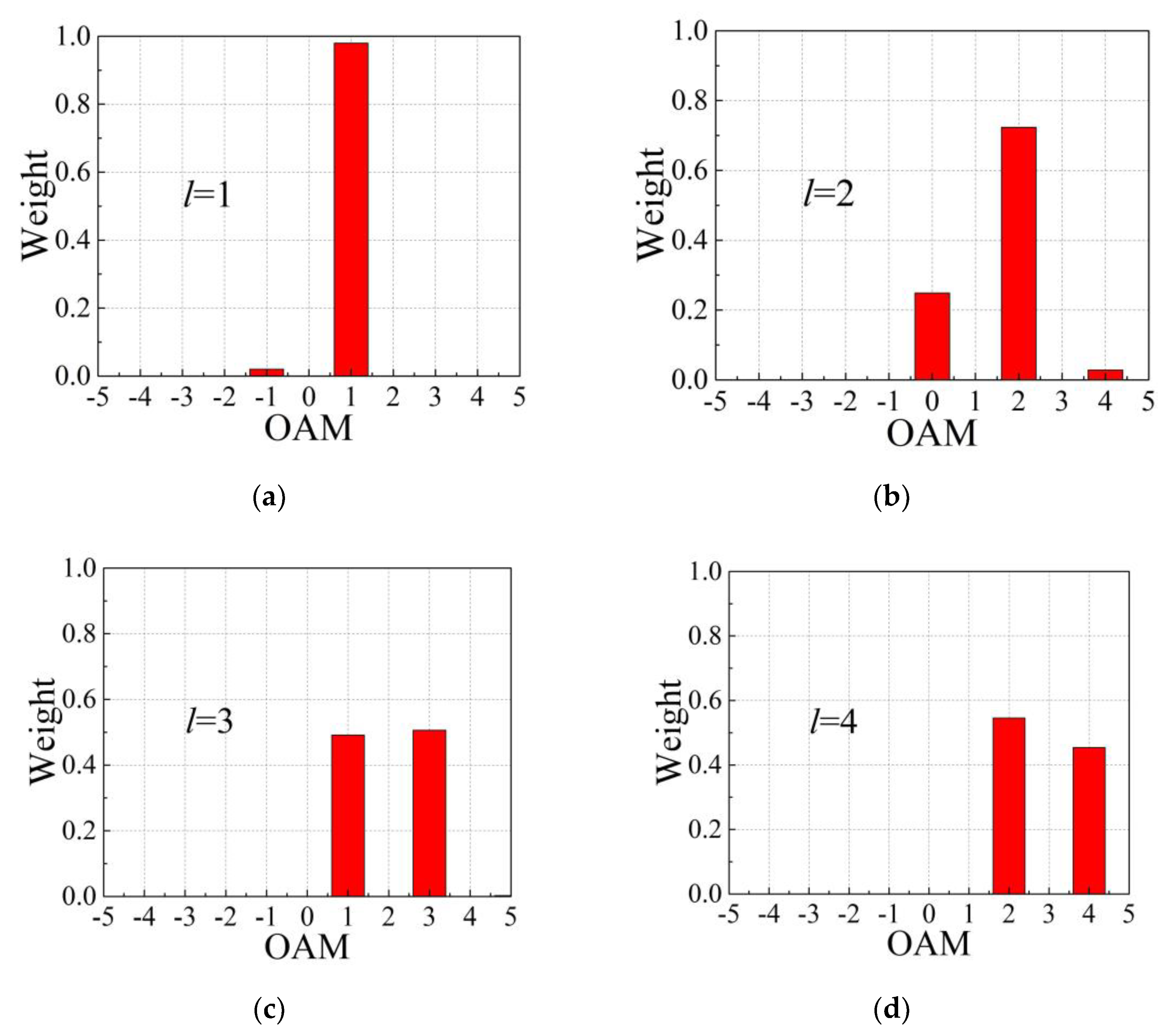
We also found that for different radii of the circle used for phase sampling, the specific phase corresponding to each sampling angle may change significantly. This is despite the same change periods of the phase within the sampling angle range. Therefore, obtaining the normalized weights of OAM modes based on the phase sampling results on a certain circle might be unstable. Furthermore, in practice, it is much easier to obtain the intensity distribution on a measurement plane, which also reflects the spatial information of the beam more comprehensively. This is the main reason that sampling is often applied on the whole measurement plane at the receiving end when the intensity and phase changes of vortex beam propagating in a turbulent environment are studied. In Figure 4, we consider sampling the entire incident field to obtain the weights of OAM modes.
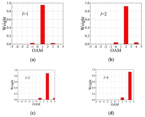
Figure 4.
Weights of the OAM modes of the incident beam with different topological charges as sampling the field on the whole measurement plane: panels (a–d) are for the topological charges of 1–4.
The electric field of the vector Bessel–Gaussian vortex beam in this manuscript is calculated based on the GLMT and ASDM. Nevertheless, the intensity distribution is not as ideal and uniform as the scalar Bessel–Gaussian vortex beam. The spiral spectrum of the incident field is also shown in Figure 4. As can be seen, the decisively dominant OAM mode clearly shows the topological charge carried by the incident beam. In addition, the modes separated by one bit from the main mode account for a small proportion. The size of the measurement plane of the field that is used to calculate the OAM modes directly affects the calculation results. The sampling plane should be large enough to ensure full reception of the beam’s energy.
Here, we further calculate the intensity and phase distributions of the scattered field of the beam that is scattered by a small spherical particle. As an example, we consider a uniform and isotropic dielectric spherical particle and set its radius and complex refractive index as a = 0.5 μm, and m = 1.377 + 1.62 × 10⁻³ i, respectively. Assuming that the measurement plane is 50 μm away from the particle center, the energy of the scattered field can be fully received if the diameter of the circular receiving plane is 2000 μm.
Figure 5 shows the intensity and phase distributions of the scattered field in the whole measurement plane. Here, the scatterer is a homogeneous and isotropic spherical particle. Panels in the first and second rows present the intensity and phase, respectively. The topological charges corresponding to the panels from left to right in each row are 1, 2, 3, and 4. The area with the concentrated intensity and the area with clear phases are small, hence, we show the results in a smaller region in the upper right corner of each panel, and the specific dimensions are marked in white. Figure 5 shows that the intensity distribution of the scattered field presents a scattered crescent shape for the topological charge 1 or 2. For all beams considered here, the scattered fields tend to rotate to the right relative to the incident fields. As for the phase distribution, for the incident beams with OAM of 1 and 3, the phases of their scattered fields at the receiving end are one topological charge, whereas the spiral direction is the opposite. In the case where the topological charge of the incident beam is l = 2, on the circumference, the phase of the scattered field remains consistent. The helical phase of the scattered field also shows two topological charges where the beam is incident with l = 4.
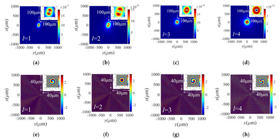
Figure 5.
The intensity and phase distributions of the scattering field of the y-polarized Bessel–Gaussian beams with different topological charges. The beam is scattered by a uniform and isotropic particle and the measurement plane is located at z = 50 μm: panels (a–d) show the intensity; and (e–h) the present phase. The corresponding topological charge from left to right is 1 to 4.
Panels (a)–(e) in Figure 6 show the one-dimensional intensity of the scattered field in the polarization direction. Figure 6f presents the phase sampling on the circumference with the location of maximum intensity as the radius. Comparing Figure 3 and Figure 6, the one-dimensional intensity distribution of the scattered field and the incident field is different, not only in the amplitude of the intensity but also in the position with the maximum intensity. For the topological charge of 2, the one-dimensional intensity of the scattered field shows a peak instead of a valley at y = 0. This phenomenon is similar to the case in which the topological charge carried by the incident beam is zero, which can also explain the phase behavior in Figure 5f. It can also be seen that when the topological charge of the incident beam is zero, the positions of the intensity peak of the incident field and scattered field remain the same, with the largest intensity at the center. Figure 6f also shows that the sampling phase on the circumference with the maximum one-dimensional intensity cannot directly and accurately reflect the phase structure of the center of the scattered field.
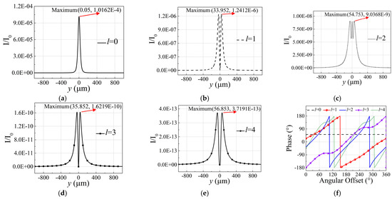
Figure 6.
(a–e) present the one-dimensional intensity of the scattered field in the polarization direction, where the beam is incident with topological charges of 0–4; (f) is the phase sampling results along the circumference. The scatterer is a uniform and isotropic spherical particle, the measurement plane is located at z = 50 μm.
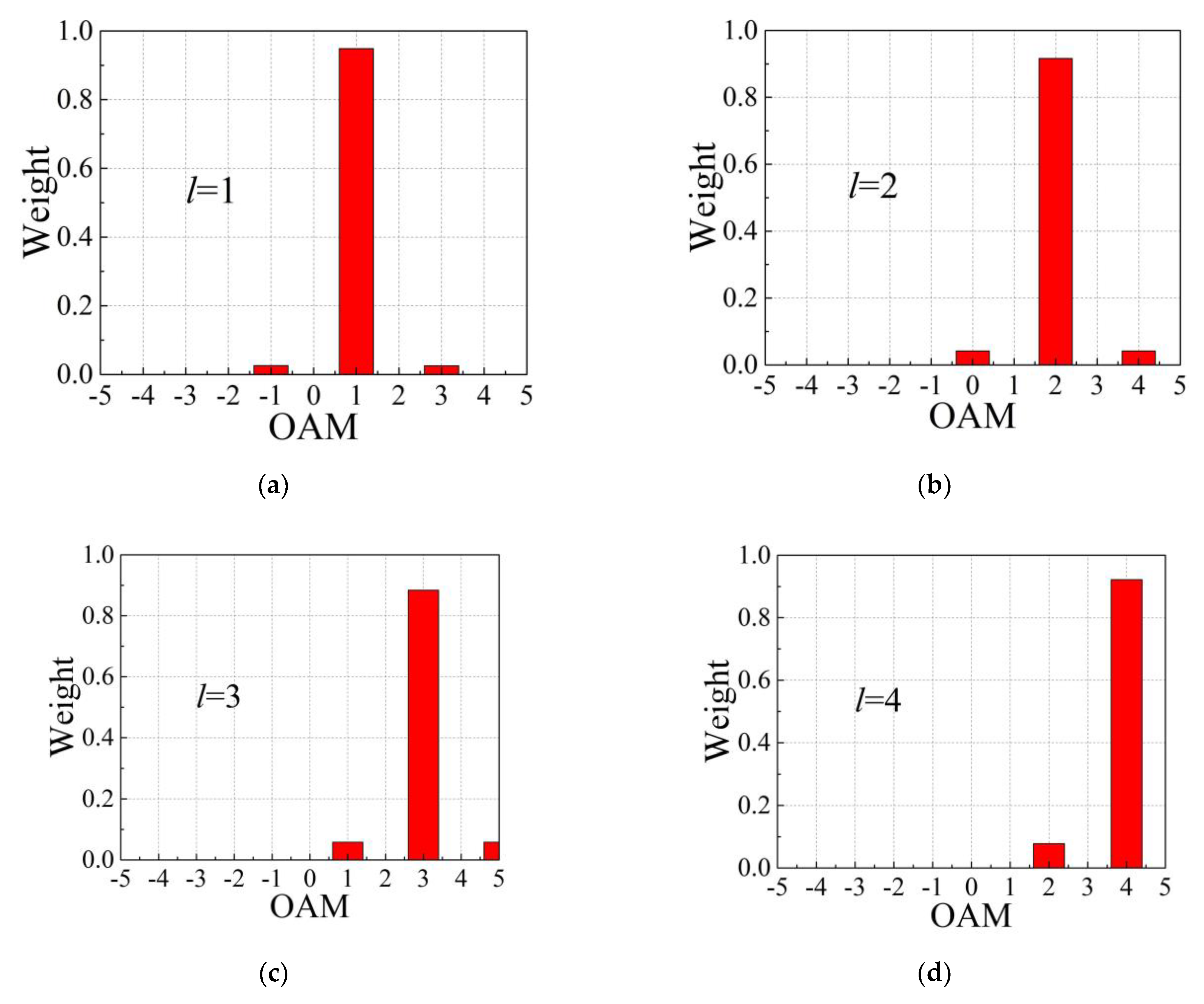
Figure 7 shows the spiral spectrum results of the entire scattered field with the measurement plane at 50 μm away from the center of the particle. The topological charge marked in the panels is the OAM mode when the beam is incident. Comparing Figure 4 and Figure 7, the spiral spectrum distribution of the scattered field is different from that of the incident field. For the incident beams with orbital angular momentums of 2, 3, and 4, the spiral spectrum of the scattered field does not show the mode of the field, but it carries the phase information of the whole scattered field. Combined with the above analysis of the sampling phase along the circle, it can be seen that sampling the whole field on the receiving plane can stably, accurately, and concretely provide the normalized weights of the OAM modes of the current beam. This can be considered as an important basis for identifying the transmission conditions.

Figure 7.
Weights of the OAM modes of the scattered field on the whole measurement plane: panels (a–d) correspond with the cases that the topological charges are 1–4, where the beam is incident. The scatterer is a uniform and isotropic spherical particle, and the measurement plane is located at z = 50 μm.
We further consider using the difference in the spiral spectrum of the scattered field at the receiving end to inverse the physicochemical parameters of the particle scatterer. Therefore, it is necessary to eliminate the possibility that the normalized weights of the OAM modes change with the transmission distance due to the calculation algorithm of the field. Figure 8 focuses on the incident beam and shows the spiral spectrum of the incident field on the receiving plane that is 50 μm away from the particle center. By comparing Figure 4 and Figure 8, can be seen that using GLMT and ASDM to calculate the beam field does not lead to a significant difference in the intensity of different sampling planes. Taking the detection probability of the OAM modes at the source as the true value, Table 1 presents the relative error between the weights of the OAM modes in Figure 4 and Figure 8. The maximum relative error is 5.99%, and the maximum magnitude of absolute error is 10−3, which is very small for the probability range 0–1. Therefore, it is reasonable to consider that the detection error of the spiral spectrum caused by the algorithm is negligible.
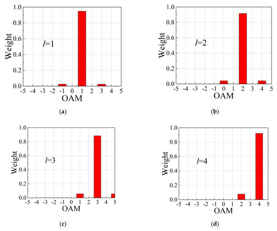
Figure 8.
The same as in Figure 4, but the measurement plane is located at z = 50 μm.

Table 1.
Relative error in the detection probability of the OAM modes at the source and at z = 50 μm for the incident field with topological charge l. Detection errors are caused by the calculation algorithm of the field.
We further investigate whether the distance between the receiving plane and the target particle affects the spiral spectrum of the scattered field of the beam. Considering the divergence of the beam, the intensity distribution of scattered field at different transmission distances is shown in Figure 9, in which the topological charge is l = 3. It can be seen that, as the transmission distance increases, the spot size of beam increases and the beam energy decreases. Therefore, when the measurement plane is set at the receiving end, the divergence of the beam needs to be fully considered, so as to avoid that the energy of field cannot be completely received due to the insufficient size of the measurement plane, and then the obtained OAM spectrum is not accurate.
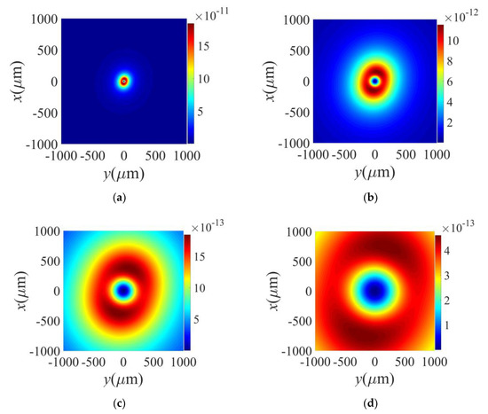
Figure 9.
The intensity distribution of the scattered field at different transmission distances, where the topological charge is l = 3 and the other parameters are the same as Figure 5: panels (a–d) correspond to the transmission distances of z = 50 μm, z = 200 μm, z = 500 μm and z = 1000 μm, respectively.
Figure 10 shows the spiral spectrum of the scattered field for the receiving plane located at z = 1000 μm. The scatterer is a homogeneous and isotropic dielectric spherical particle. Compared with Figure 7 and the relative error between them is shown in Table 2, where the detection probability of the OAM modes of the scattered field at z = 50 μm is set to the true value. It is seen that the maximum relative error is 6.38%, and the maximum magnitude of absolute error is 10−3. Therefore, the position of the receiving plane in the far region does not affect the spiral spectrum of the scattered fields.
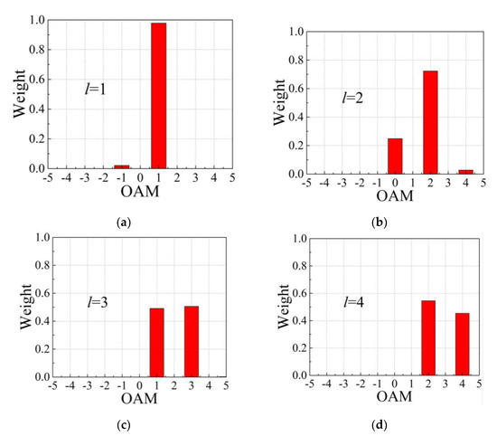
Figure 10.
The same as in Figure 7, but the measurement plane is located at z = 1000 μm.
Table 2.
Relative error in the detection probability of the OAM modes for scattered fields at z = 50 μm and z = 1000 μm of the beam with topological charge l. The scatterer is a uniform and isotropic dielectric sphere.
In practice, the beam continues propagating forward after being scattered by particles. Therefore, the field received by the measurement plane set in the far region needs to be the total external field, hence the summation of the scattered field and the incident field. Therefore, it is necessary to study the normalized weights of the OAM modes of the total external field. Figure 11 shows the intensity and phase distribution of the total external field in the far region after the beam is scattered by a homogeneous and isotropic spherical particle. The location of the measurement plane is z = 50 μm. Compared with the incident field and scattered field, the phase distribution of the total external field is very irregular, and the OAM mode mixing is more obvious. From the intensity amplitude of the field, it can be seen that the energy of the incident beam has been substantially reduced if it is transmitted to the position at which the receiving plane is located.
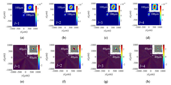
Figure 11.
The same as in Figure 5, but the total field in the far region is considered.
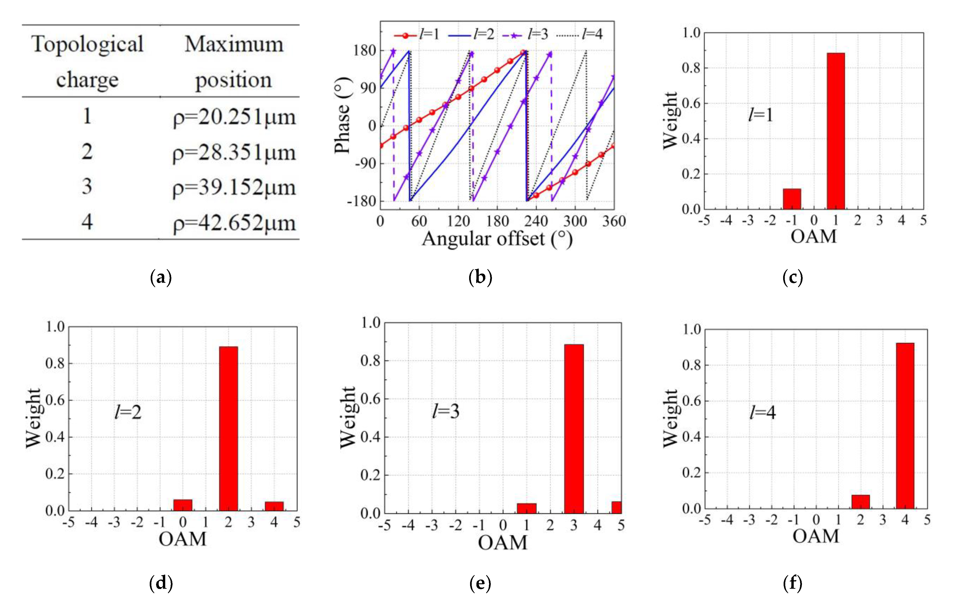
Figure 12 shows the position of the maximum intensity of the total external field in the polarization direction (Figure 12a), the sampling phase on the circumference where the maximum is located (Figure 12b), and the spiral spectrum results of the whole external field (Figure 12c–f). Compared with the results of the incident beam shown in Figure 3 and Figure 4, the maximum one-dimensional intensity of the external field after scattering is significantly changed. The phase corresponding to the sampling angle along the circumference is different. However, the phase along the circle within the whole sampling range still shows the OAM mode carried by the incident beam. This is the case even if the phase structure of the external field becomes extremely irregular. There is a weight difference between the spiral spectrum of the external field and that of the incident field. It can be seen that the larger the topological charge of the incident beam, the smaller the difference. This is because the beam is incident on the axis, so the lower the energy irradiates on the particle when the topological charge is larger, the weaker the scattering effect and the smaller the proportion of the scattered field in the total external field.

Figure 12.
The information of the external field in the far region after the beam is scattered by a uniform and isotropic spherical particle: (a) lists the position of the maximum intensity of the corresponding external field in the polarization direction where the beam is incident with a different topological charge; (b) shows the sampling phase along the circle where the maximum lies; and (c–f) are the spiral spectra of the entire external fields. The measurement plane is located at z = 50 μm.
The above analysis shows that the weights of OAM modes in both scattered and external fields at the receiving end are different from that of the incident field. This enables significant application opportunities, where the spiral spectrum of the field on the measurement plane can be used as a reference for retrieving the physicochemical parameters of the scatterer particle. In addition, sampling the phase along the circumference can only show the phase performance of the intensity on a certain sampling radius, hence unable to reflect the deformation of the OAM states of the whole field.
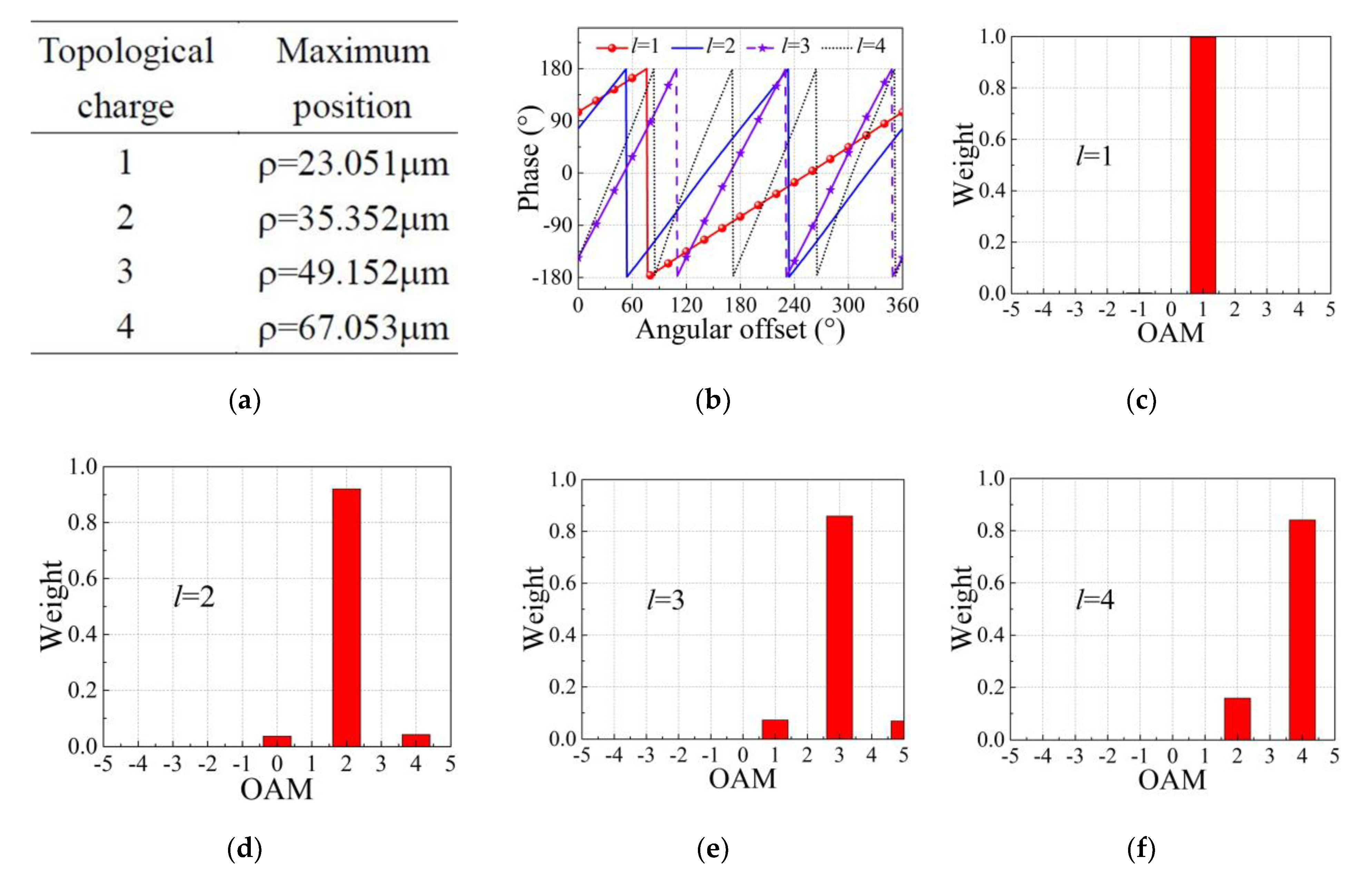
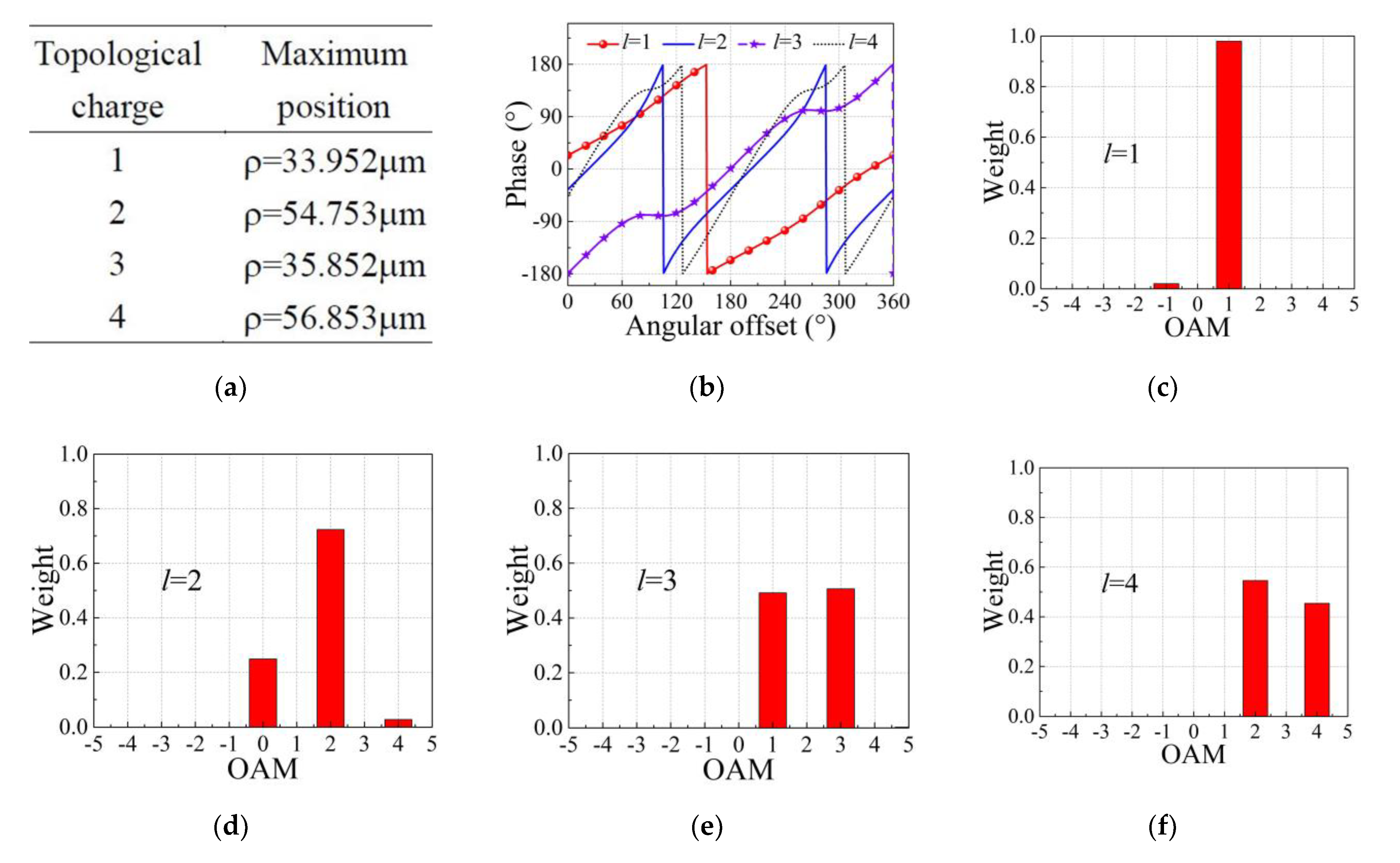
To show that the spiral spectrum can identify the parameters of the scatterer particle, we use the single variable method and provide the following examples. Here, we change the particle radius from 0.5 μm to 1.0 μm and show the simulation results in Figure 13. The specific information of each panel in Figure 13 is the same as in Figure 12. Similarly, Figure 14 includes the simulations after changing the complex reflective index of the particle to m = 1.75 + 0.44i. A comparison of the results in Figure 13 and Figure 14 with Figure 6 and Figure 7 show clear differences in the position of maximum intensity, the sampling phase along a circle, and the spiral spectrum distribution. Therefore, the inversion of particle parameters by using the weights of the OAM modes of the scattered field at the receiving end is theoretically viable. Nevertheless, because the change of different types of parameters may lead to the same spiral spectrum simulation results, it might be much more accurate to use both the circumferential sampling phase and the spiral spectrum to inverse the particle parameters.
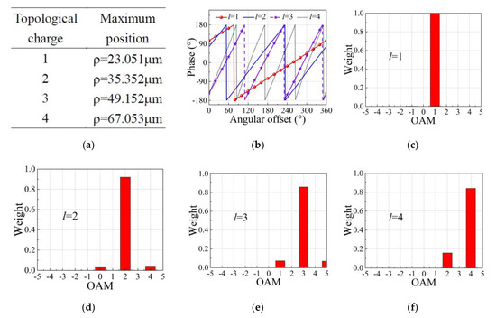
Figure 13.
The same as in Figure 12, but here the scattered field is simulated. The radius of the illuminated particle is changed to 1.0 μm and other parameters are unchanged.
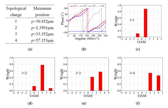
Figure 14.
The same as in Figure 12, but simulating the scattered field. The complex refractive index of the scatterer particle is changed to m = 1.75 + 0.44i, and other parameters are unchanged.
Similarly, the particle parameters can also be retrieved by using the circumferential sampling phase and the spiral spectrum of the total external field at the receiving end.
We further change the properties of the scatterer and replace it with a charged spherical particle. The surface electrostatic potential is 50 V and the temperature is 30 ℃, reflecting the amount of charge carried on the particle. The simulation results are shown in Figure 15. Comparing Figure 15 with Figure 6 and Figure 7, we can see that the results of one-dimensional intensity, sampling phase along a circle, and spiral spectrum of the scattered field of a charged spherical particle are consistent with those of a neutral dielectric sphere. The reason is that when the particle size is small enough, the scattering effect of a charged spherical particle is different from that of a neutral one, and the difference is more obvious in the near region than in the far region. Therefore, the scattered field in the far region can hardly identify whether the scatterer particle carries charges or not. Similarly, the external field in the far region is unable to identify this.

Figure 15.
The same as in Figure 12, with the simulated scattered field. The scatterer is changed into a charged particle where other parameters remain unchanged. The surface electrostatic potential of the charged particle is φ = 50 V and the surface temperature is T = 30 ℃.
Finally, we discuss whether other types of vector Bessel–Gaussian vortex beams can show the differences in the weights of OAM modes for various characteristic parameters of particles. Here, we consider the right circular polarization and the radial polarization. Their field distributions in the x-direction at the receiving end are used to analyze the spiral spectrum characteristics in order to explore whether we can obtain the spiral spectrum varying with the parameters of the scatterer particle only, based on knowing the component field in a certain direction. Hence, the characteristic parameters of the scatterer can be retrieved according to the differences in the spiral spectrum. This may then be used for remote sensing applications in engineering.
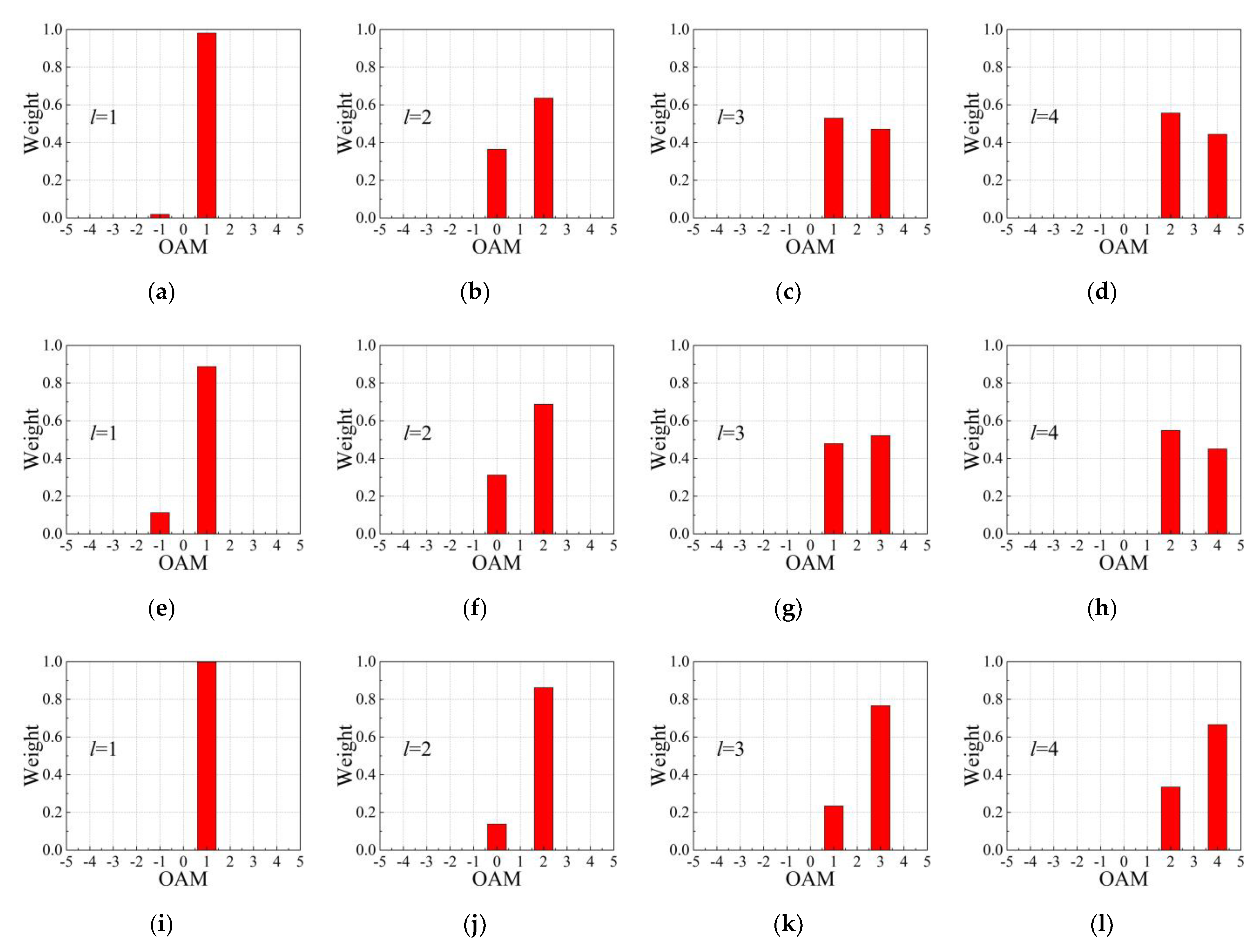
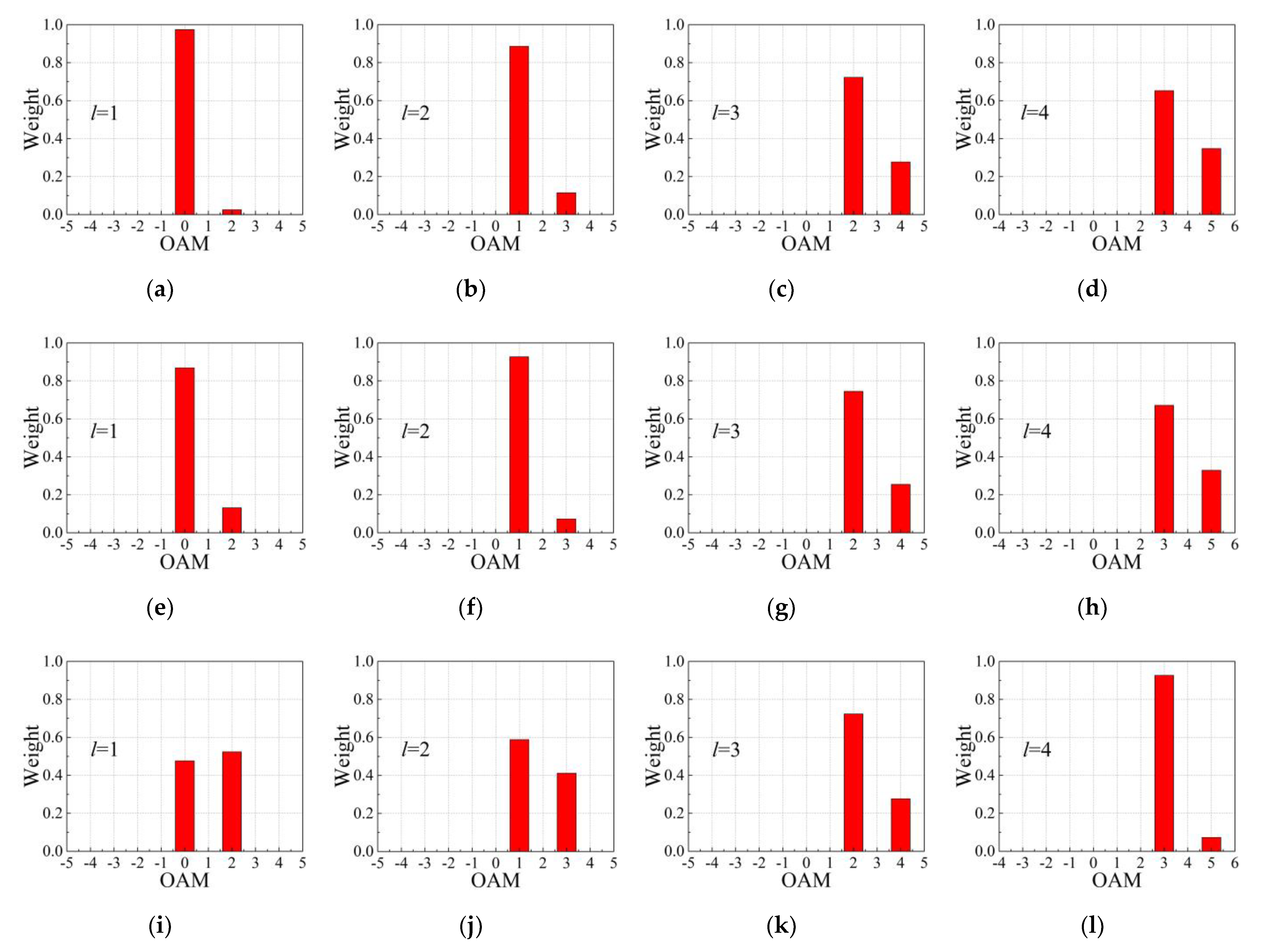
Figure 16 shows the spiral spectrum of the scattered field of the right circular polarized Bessel–Gaussian vortex beam. The topological charges 1-4 are considered, corresponding to the panels from left to right in each row. The radius a, and the complex refractive index m, of the irradiated particle in each row are different. In the first row, a = 0.5 μm and m = 1.377 + 1.62 × 10⁻³i, in the second, a = 0.5 μm and m = 1.75 + 0.44i and a = 1.0 μm and m = 1.377 + 1.62 × 10⁻³i in the third row. The particle is homogeneous and isotropic. The spiral spectrum distribution of the scattered field of the right circular polarized Bessel–Gaussian vortex beam in the x-direction is highly sensitive to the change of the characteristic parameters of the illuminated particle. Instances of such parameters are the complex refractive index and size of the particle. In other words, for the right circular polarized Bessel–Gaussian vortex beam, the characteristic parameters of the scatterer particle can be retrieved by using the spiral spectrum of the scattered field in the x-direction. In addition, comparing the results of the first and the third rows, it can be seen that the particle size is larger, the weight of the primary mode becomes dominant, which visually shows the OAM state carried by the incident beam.
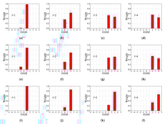
Figure 16.
The spiral spectra of the scattering fields of right circular polarized Bessel–Gaussian vortex beams were scattered by a particle with different sizes and different complex refractive indices. The scatterer particle is a uniform and isotropic sphere. Radius a and complex refractive index m of the illuminated particle are: a = 0.5 μm and m = 1.377 + 1.62 × 10⁻³i in panels (a–d); a = 0.5 μm and m = 1.75 + 0.44i in panels (e–h); a = 1.0 μm and m = 1.377 + 1.62 × 10⁻³i in panels (i–l). The corresponding topological charge from left to right in each row is 1–4.
Similar to Figure 16, Figure 17 discusses the simulation results where the incident beam is a radial polarized Bessel–Gaussian vortex beam. Refer to Figure 16 for specific contents and parameters of panels. As it is seen, variations in the characteristic parameters of the scatterer particle also affect the spiral spectrum distribution of the scattered field of radial polarized Bessel–Gaussian vortex beam.
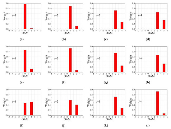
Figure 17.
The same as in Figure 16, but the radial polarization is considered.
The above discussions show that changing the characteristic parameters of the illuminated particle significantly alters the spiral spectrum of the scattered field of the vector Bessel–Gaussian vortex beam. Therefore, for detecting parameters of the particle, one can select Bessel–Gaussian vortex beams with different polarization states for incidence. Fields in multiple directions can be then sampled and their spiral spectrum characteristics can be analyzed to build a multi-dimensional database. Similarly, a uniform and isotropic dielectric sphere can be used as an auxiliary objet. By changing the multiple characteristic parameters of this object, a multi-dimensional database can be then established to identify the parameters of the incident vector Bessel–Gaussian beam. The higher the number of such dimensions, the more accurate the inversion results of the beam and particle parameters. In our future research, we will investigate whether a similar method can be extended to other shaped beams and irregular scatterers.
4. Conclusions
We investigated the impact of the scattering effect of a spherical particle on the orbital angular spectrum of a vector Bessel–Gaussian vortex beam. We considered y polarization, right circular polarization, and radial polarization. The generalized Lorenz–Mie theory and the angular spectrum decomposition method were used to describe the scattered and external fields of vector Bessel–Gaussian vortex beam in the far-field region. The spiral spectrum expansion method was then combined to simulate the orbital angular momentum spectra of scattered and external fields. The calculation algorithm of the field does not cause the spiral spectrum of the beam change with the position of the measurement plane. Our simulation results further suggested that sampling along the circumference cannot fully reflect the phase information of the field, and different sampling radii lead to different sampling results. The spiral spectra of the scattered and external fields of y polarized, right circular polarized, and radial polarized Bessel–Gaussian vortex beams are sensitive to the changes in the particle characteristic parameters, such as its complex refractive index and size. The sampling results are inconsistent in different directions. Therefore, the polarization state of the beam and sampling direction of the field can be used as calculation dimensions to build a database for retrieving the parameters of scattered particles. Similarly, the characteristics of the incident beam can be retrieved by using the particle parameters. Studying the field distribution and spiral spectrum of the vector Bessel–Gaussian vortex beam scattered by spherical particles provides a theoretical basis for potential applications of vortex beam in remote sensing, such as the real-time monitoring of rain droplet size in rainy environments.
Author Contributions
Conceptualization, M.C., L.G., M.P.J.L., P.W. and S.L.; methodology, C.S., M.C., M.P.J.L., R.L. and S.L.; software, C.S. and R.L.; investigation; C.S., M.C. and S.L.; resources, L.G., J.L. and P.W.; writing—original draft preparation; C.S. and M.C.; writing—review and editing, M.C., L.G., M.P.J.L. and J.L. All authors have read and agreed to the published version of the manuscript.
Funding
This research was supported by the National Natural Science Foundation of China (Grant No. U20B2059, 61627901, 61901336, 61905186), the Foundation for Innovative Research Groups of the National Natural Science Foundation of China (Grant No. 61621005), the Fundamental Research Funds for the Central Universities (Grant No. YJS2208, QTZX22037).
Institutional Review Board Statement
Not applicable.
Informed Consent Statement
Not applicable.
Data Availability Statement
Not applicable.
Acknowledgments
The authors would like to thank the editor and anonymous reviewers who handled our paper.
Conflicts of Interest
The authors declare no conflict of interest.
Appendix A
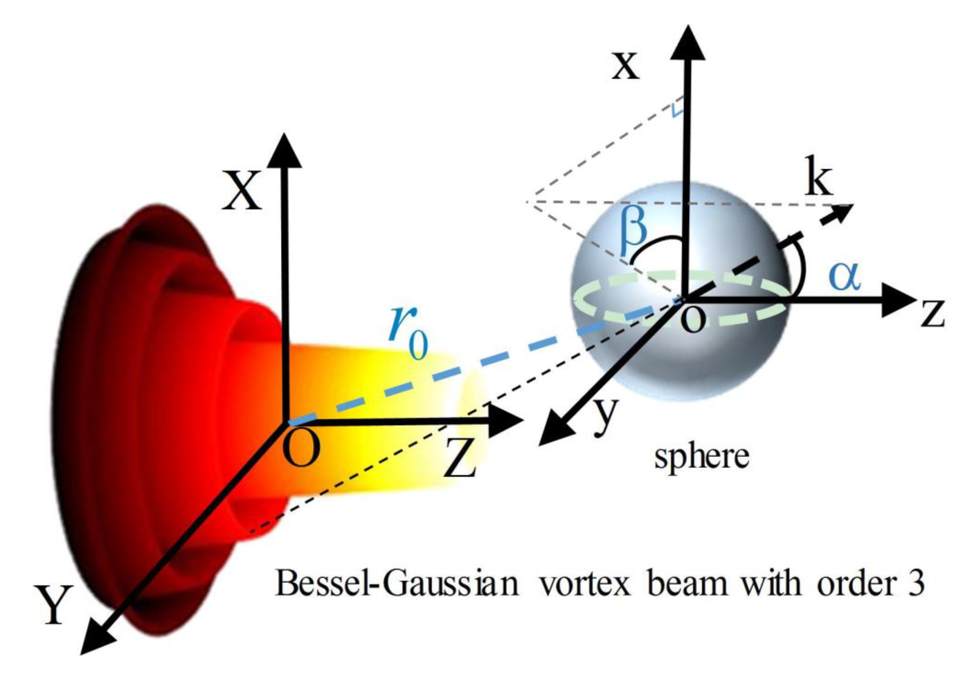
Considering a spherical particle with radius a and relative complex refractive index m illuminated by a vector Bessel–Gaussian vortex beam. The coordinate systems of the particle and beam are o-xyz and O-XYZ, respectively (Figure A1). Here, α is the angle between the wave vector k of the plane wave component and the transmission axis Z, and β is the azimuthal angle. The coordinates of the beam center O in the particle coordinate system are (x0, y0, z0) indicating the relative position of the beam and particle.

Figure A1.
Schematic diagram of a spherical object illuminated by a Bessel–Gaussian vortex beam.
Figure A1.
Schematic diagram of a spherical object illuminated by a Bessel–Gaussian vortex beam.
The expression of the electric field of a vector Bessel–Gaussian beam with order l at the source plane is
where, , , θb is the conic angle and . w0 is the waist radius of the incident beam, is the Bessel function of order l. represents the vector state of the beam and the subscript u indicates the polarization type.
In the angular spectrum theory of light, the light field on any plane can be considered as a linear superposition of many plane waves with different amplitudes and propagation directions. Therefore, from the definition, Equation (A1) can be expressed as
where, , , and . Using straightforward mathematical transformations, the derivation result of Equation (A2) is
is the modified Bessel function of order l. For the details of the derivation process, see [40].
For a beam on an arbitrary plane, the expression of the electric field changes to
Taking the beam position into account, i.e., the beam’s location is (x0, y0, z0) instead of (0, 0, 0). Correspondingly, the above equation becomes
In Equation (A5), , , . It can be expanded by using the vector spherical wave functions as
where
Comparing the expression of the electric field in Equation (A6) with Equation (1), the mathematical relationship between the beam shape coefficients ( and ) and the expansion coefficients ( and ) can be obtained.
In the simulation part, y, right circular, and radial polarization are discussed. Therefore, the derivation results of the beam shape coefficients for these three polarization states are given.
- Y polarizationwhere
- Right circular polarizationThe expressions of and are consistent with those of the y polarization state.
- Radial polarization
References
- Allen, L.; Beijersbergen, M.W.; Spreeuw, R.J.; Woerdman, J.P. Orbital angular momentum of light and the transformation of Laguerre-Gaussian laser modes. Phys. Rev. A 1992, 45, 8185–8189. [Google Scholar] [CrossRef] [PubMed]
- Otte, E.; Denz, C. Optical trapping gets structure: Structured light for advanced optical manipulation. Appl. Rhys. Rev. 2020, 7, 041308. [Google Scholar] [CrossRef]
- Wang, J.; Liu, K.; Cheng, Y.; Wang, H. Vortex SAR imaging method based on OAM beams design. IEEE Sens. J. 2019, 19, 11873–11879. [Google Scholar] [CrossRef]
- Wang, J.; Yang, J.; Fazal, I.; Ahmed, N.; Yan, Y.; Huang, H.; Ren, Y.; Yue, Y.; Dolinar, S.; Tur, M.; et al. Terabit free-space data transmission employing orbital angular momentum multiplexing. Nat. Photonics 2012, 6, 488–496. [Google Scholar] [CrossRef]
- Wang, J.; Liu, J.; Li, S.; Zhao, Y.; Du, J.; Zhu, L. Orbital angular momentum and beyond in free-space optical communications. Nanophotonics 2022, 11, 645–680. [Google Scholar] [CrossRef]
- Willner, A.; Pang, K.; Song, H.; Zou, K.; Zhou, H. Orbital angular momentum of light for communications. Appl. Phys. Rev. 2021, 8, 041312. [Google Scholar] [CrossRef]
- Gong, L.; Zhao, Q.; Zhang, H.; Hu, X.; Huang, K.; Yang, J.; Li, Y. Optical orbital-angular-momentum-multiplexed data transmission under high scattering. Light Sci. Appl. 2019, 8, 27. [Google Scholar] [CrossRef]
- Zhang, C.; Chen, D. Large-scale orbital angular momentum radar pulse generation with rotational antenna. IEEE Antennas Wirel. Propag. Lett. 2017, 16, 2316–2319. [Google Scholar] [CrossRef]
- Barbuto, M.; Alù, A.; Bilotti, F.; Toscano, A. Dual-circularly polarized topological patch antenna with pattern diversity. IEEE Access 2021, 9, 48769–48776. [Google Scholar] [CrossRef]
- Liu, K.; Li, X.; Gao, Y.; Cheng, Y.; Wang, H.; Qin, Y. High-resolution electromagnetic vortex imaging based on sparse bayesian learning. IEEE Sens. J. 2017, 17, 6918–6927. [Google Scholar] [CrossRef]
- Lin, M.; Gao, Y.; Liu, P.; Liu, J. Super-resolution orbital angular momentum based radar targets detection. Electron. Lett. 2016, 52, 1168–1170. [Google Scholar] [CrossRef]
- Wang, W.; Gozali, R.; Shi, L.; Lindwasser, L.; Alfano, R. Deep transmission of Laguerre-Gaussian vortex beams through turbid scattering media. Opt. Lett. 2016, 41, 2069–2072. [Google Scholar] [CrossRef] [PubMed]
- Tang, B.; Bai, J.; Sheng, X. Orbital-angular-momentum-carrying wave scattering by the chaff clouds. IET Radar Sonar Nav. 2018, 12, 649–653. [Google Scholar]
- Torner, L.; Torres, J.; Carrasco, S. Digital spiral imaging. Opt. Express 2005, 13, 873–881. [Google Scholar] [CrossRef]
- Wang, Y.; Bai, L.; Xie, J.; Zhang, D.; Lv, Q.; Guo, L. Spiral spectrum of high-order elliptic Gaussian vortex beams in a non-Kolmogorov turbulent atmosphere. Opt. Express 2021, 29, 16056–16072. [Google Scholar] [CrossRef]
- Wang, A.; Zhu, L.; Deng, M.; Lu, B.; Guo, X. Experimental demonstration of OAM-based transmitter mode diversity data transmission under atmosphere turbulence. Opt. Express 2021, 29, 13171–13182. [Google Scholar] [CrossRef]
- Li, J.; Chen, X.; McDuffie, S.; Najjar, M.; Rafsanjani, S.; Korotkova, O. Mitigation of atmospheric turbulence with random light carrying OAM. Opt. Commun. 2019, 446, 178–185. [Google Scholar] [CrossRef]
- Klug, A.; Nape, I.; Forbes, A. The orbital angular momentum of a turbulent atmosphere and its impact on propagating structured light fields. New J. Phys. 2021, 23, 093012. [Google Scholar] [CrossRef]
- Ferlic, N.; Iersel, M.; Davis, C. Weak turbulence effects on different beams carrying orbital angular momentum. J. Opt. Soc. Am. A 2021, 38, 1423–1437. [Google Scholar] [CrossRef]
- Watkins, R.; Dai, K.; White, G.; Li, W.; Miller, J.; Morgan, K.; Johnson, E. Experimental probing of turbulence using a continuous spectrum of asymmetric OAM beams. Opt. Express 2020, 28, 924–935. [Google Scholar] [CrossRef]
- Porfirev, A.; Kirilenko, M.; Khonina, S.; Skidanov, R.; Soifer, V. Study of propagation of vortex beams in aerosol optical medium. Appl. Opt. 2017, 56, E8–E15. [Google Scholar] [CrossRef] [PubMed]
- Baghdady, J.; Miller, K.; Morgan, K.; Byrd, M.; Osler, S.; Ragusa, R.; Li, W.; Cochenour, B.; Johnson, E. Multi-gigabit/s underwater optical communication link using orbital angular momentum multiplexing. Opt. Express 2016, 24, 9794–9805. [Google Scholar] [CrossRef] [PubMed]
- Deng, S.; Yang, D.; Zhang, Y. Capacity of communication link with carrier of vortex localized wave in absorptive turbulent seawater. Waves Random Complex Media 2020, 12, 1–14. [Google Scholar] [CrossRef]
- Yang, H.; Yan, Q.; Wang, P.; Hu, L.; Zhang, Y. Bit-error rate and average capacity of an absorbent and turbulent underwater wireless communication link with perfect Laguerre-Gauss beam. Opt. Express 2022, 30, 9053–9064. [Google Scholar] [CrossRef]
- Wang, W.; Wang, P.; Pang, W.; Pan, Y.; Nie, Y.; Guo, L. Evolution properties and spatial-mode UWOC performances of the perfect vortex beam subject to oceanic turbulence. IEEE Trans. Commun. 2021, 69, 7647–7658. [Google Scholar] [CrossRef]
- Petrov, D.; Rahuel, N.; Molina-Terriza, G.; Torner, L. Characterization of dielectric spheres by spiral imaging. Opt. Lett. 2012, 37, 869–871. [Google Scholar] [CrossRef]
- Li, H.; Honary, F.; Wu, Z.; Shang, Q.; Bai, L. Reflection, transmission, and absorption of vortex beams propagation in an inhomogeneous magnetized plasma slab. IEEE Trans. Antennas Propag. 2018, 66, 4194–4201. [Google Scholar] [CrossRef]
- Liu, K.; Liu, H.; Sha, W.; Cheng, Y.; Wang, H. Backward scattering of electrically large standard objects illuminated by OAM Beams. IEEE Antennas Wirel. Propag. Lett. 2020, 19, 1167–1171. [Google Scholar] [CrossRef]
- Mcgloin, D.; Dholakia, K. Bessel beams: Diffraction in a new light. Contemp. Phys. 2005, 46, 15–28. [Google Scholar] [CrossRef]
- Akram, M.; Mehmood, M.; Tauqeer, T.; Rana, A.; Rukhlenko, I.; Zhu, W. Highly efficient generation of Bessel beams with polarization insensitive metasurfaces. Opt. Express 2019, 27, 9467–9480. [Google Scholar] [CrossRef]
- Aiello, A.; Agarwal, G. Wave-optics description of self-healing mechanism in Bessel beams. Opt. Lett. 2014, 39, 6819–6822. [Google Scholar] [CrossRef] [PubMed]
- Chu, X. Analytical study on the self-healing property of Bessel beam. Eur. Phys. J. D 2012, 66, 1–5. [Google Scholar] [CrossRef]
- Gatto, A.; Tacca, M.; Martelli, P.; Boffi, P.; Martinelli, M. Free-space orbital angular momentum division multiplexing with Bessel beams. J. Opt. 2011, 13, 064018. [Google Scholar] [CrossRef]
- Eyyuboğlu, H. Propagation of higher order Bessel-Gaussian beams in turbulence. Appl. Phys. B 2007, 88, 259–265. [Google Scholar] [CrossRef]
- Lukin, I. Integral momenta of vortex Bessel-Gaussian beams in turbulent atmosphere. Appl. Opt. 2016, 55, B61–B66. [Google Scholar] [CrossRef] [PubMed]
- Xu, Y.; Zhang, Y. Bandwidth-limited orbital angular momentum mode of Bessel Gaussian beams in the moderate to strong non-Kolmogorov turbulence. Opt. Commun. 2019, 438, 90–95. [Google Scholar] [CrossRef]
- Vyas, S.; Kozawa, Y.; Sato, S. Self-healing of tightly focused scalar and vector Bessel-Gauss beams at the focal plane. J. Opt. Soc. Am. A 2011, 28, 837–843. [Google Scholar] [CrossRef]
- Li, P.; Zhang, Y.; Liu, S.; Cheng, H.; Han, L.; Wu, D.; Zhao, J. Generation and self-healing of vector Bessel-Gauss beams with variant state of polarizations upon propagation. Opt. Express 2017, 25, 5821–5831. [Google Scholar] [CrossRef]
- Huang, K.; Shi, P.; Cao, G.; Li, K.; Zhang, X.; Li, Y. Vector-vortex Bessel-Gauss beams and their tightly focusing properties. Opt. Lett. 2011, 36, 888–890. [Google Scholar] [CrossRef]
- Shi, C.; Guo, L.; Cheng, M.; Li, R. Scattering of a high-order vector Bessel Gaussian beam by a spherical marine aerosol. J. Quant. Spectrosc. Radiat. Transf. 2021, 265, 107552. [Google Scholar] [CrossRef]
- Shi, C.; Cheng, M.; Guo, L.; Li, R.; Li, J. Attenuation characteristics of Bessel Gaussian vortex beam by a wet dust particle. Opt. Commun. 2022, 514, 128138. [Google Scholar] [CrossRef]
- Gouesbet, G.; Gréhan, G. Generalized Lorenz-Mie Theories; Springer: Berlin/Heidelberg, Germany, 2011; pp. 50–55. [Google Scholar]
- Zambrana-Puyalto, X.; Molina-Terriza, G. The role of the angular momentum of light in Mie scattering. Excitation of dielectric spheres with Laguerre-Gaussian modes. J. Quant. Spectrosc. Radiat. Transf. 2013, 126, 50–55. [Google Scholar] [CrossRef]
- Bohren, C.; Huffman, D. Absorption and Scattering of Light by Small Particles; Wiley: New York, NY, USA, 1983; p. 100. [Google Scholar]
- Klačka, J.; Kocifaj, M. Scattering of electromagnetic waves by charged spheres and some physical consequences. J. Quant. Spectrosc. Radiat. Transf. 2007, 106, 170–183. [Google Scholar] [CrossRef]
- Kocifaj, M.; Klačka, J. Scattering of electromagnetic waves by charged spheres: Near-field external intensity distribution. Opt. Lett. 2012, 37, 265–267. [Google Scholar] [CrossRef] [PubMed]
- Ou, J.; Jiang, Y.; Zhang, J.; Tang, H.; He, Y.; Wang, S.; Liao, J. Spreading of spiral spectrum of Bessel-Gaussian beam in non-Kolmogorov turbulence. Opt. Commun. 2014, 318, 95–99. [Google Scholar] [CrossRef]
- Sztul, H.; Alfano, R. The Poynting vector and angular momentum of Airy beams. Opt. Express 2008, 16, 9411–9416. [Google Scholar] [CrossRef] [PubMed]
- Jiang, Y.; Wang, S.; Zhang, J.; Ou, J.; Tang, H. Spiral spectrum of Laguerre-Gaussian beam propagation in non-Kolmogorov turbulence. Opt. Commun. 2013, 303, 38–41. [Google Scholar] [CrossRef]
- Yao, E.; Franke-Arnold, S.; Courtial, J.; Barnett, S.; Padgett, M. Fourier relationship between angular position and optical orbital angular momentum. Opt. Express 2006, 14, 9071–9076. [Google Scholar] [CrossRef]
- Jack, B.; Padgett, M.; Franke-Arnold, S. Angular diffraction. New J. Phys. 2008, 10, 103013. [Google Scholar] [CrossRef]
- Yang, L.; Sun, S.; Sha, W. Ultrawideband reflection-type metasurface for generating integer and fractional orbital angular momentum. IEEE Trans. Antennas Propag. 2020, 68, 2166–2175. [Google Scholar] [CrossRef] [Green Version]


Publisher’s Note: MDPI stays neutral with regard to jurisdictional claims in published maps and institutional affiliations. |
© 2022 by the authors. Licensee MDPI, Basel, Switzerland. This article is an open access article distributed under the terms and conditions of the Creative Commons Attribution (CC BY) license (https://creativecommons.org/licenses/by/4.0/).