On the Accuracy and Consistency of Quintuple Collocation Analysis of In Situ, Scatterometer, and NWP Winds

Abstract

The accuracy and consistency of a quintuple collocation analysis of ocean surface vector winds from buoys, scatterometers, and NWP forecasts is established. A new solution method is introduced for the general multiple collocation problem formulated in terms of covariance equations. By a logarithmic transformation, the covariance equations reduce to ordinary linear equations that can be handled using standard methods. The method can be applied to each determined or overdetermined subset of the covariance equations. Representativeness errors are estimated from differences in spatial variances. The results are in good agreement with those from quadruple collocation analyses reported elsewhere. The geometric mean of all solutions from determined subsets of the covariance equations equals the least-squares solution of all equations. The accuracy of the solutions is estimated from synthetic data sets with random Gaussian errors that are constructed from the buoy data using the values of the calibration coefficients and error variances from the quintuple collocation analysis. For the calibration coefficients, the spread in the models is smaller than the accuracy, but for the observation error variances, the spread and the accuracy are about equal only for representativeness errors evaluated at a scale of 200 km for $u$ and 100 km for $v$. Some average error covariances differ significantly from zero, indicating weak inconsistencies in the underlying error model. Possible causes for this are discussed. With a data set of 2454 collocations, the accuracy in the observation error standard deviation is 0.02 to 0.03 m/s at the one-sigma level for all observing systems.

1. Introduction

The triple collocation method was introduced by Stoffelen [1] in order to assess the intercalibration coefficients and error variances of three systems observing ocean surface vector winds. It is an extension of regression analysis to three dimensions under the assumptions that linear calibration is sufficient, the errors are random and independent of the measured value (also referred to as error orthogonality), and the correlations in the errors of the observing systems are known or can be neglected. Triple collocation has been applied to a variety of geophysical parameters such as ocean surface vector winds [2,3], ocean surface wind speed [4], ocean surface current [5], sea surface salinity [6], precipitation [7,8], soil moisture [9,10], etc. The list is far from exhaustive and the reader is referred to the references and the references therein.

Stoffelen [1] already realized that the assumption of uncorrelated errors is, in most cases, violated because differences in the spatial and/or temporal resolutions between the observation systems give rise to representativeness errors which express themselves as error covariances; also, in cases where the measurements are completely independent. Unfortunately, the term representativeness error has different meanings in different communities [11]. In this paper, we follow the meteorological convention and consider representativeness errors as caused by differences in resolution between the various systems in order to distinguish them from error correlations caused by interdependence of the measurement system errors. Spatial representativeness errors can be estimated from spectral analysis [1,2], constraints on the intercalibration [12], or spatial analysis [13]. Another approach is to estimate spatial representativeness errors, or error covariances in general, using more than three observation systems. This is enabled by the increase in satellite observations, but can also be achieved by introducing instrumental variables, i.e., using model forecasts or hindcasts with different analysis times [4,5,14] or time-lagged variables [15]. These developments led to so-called extended collocation analyses, although that term has also been used in [16] for a generalization of the correlation coefficient from linear regression to triple collocation.

A number of methods has been proposed to solve the multiple collocation problem for four or more observing systems. The methods depend on the spatial and temporal statistical properties of the quantity under consideration and on the availability of a calibration reference. The most popular one is to change variables, cast the problem in matrix form, and solve the resulting overdetermined system of equations using a least-squares method [9,17]. This is equivalent to minimizing a quadratic cost function for the unknowns. A different approach has been followed in [3] for quadruple collocations where each subset of four equations from the six off-diagonal covariance equations is solved analytically. There are 15 such subsets, further referred to as models, of which 12 are soluble. The remaining two equations of each soluble model can be solved for two error covariances. The number of possibilities grows rapidly with the number of observing systems, and for quintuple collocation there are already 252 models. It is clear that the analytical solution of the problem becomes increasingly cumbersome.

In [3], it was found that different models give different solutions, and the question arises whether these differences are due to statistical noise or to inconsistencies in the underlying error model. This question can best be answered in a quintuple or higher collocation analysis in order to have better statistics over the models. Two more things are needed to obtain an answer: an efficient method to solve the covariance equations for all models and a method to estimate the accuracy of the solutions.

In this paper, a new method is introduced for solving all possible models. The error variances of the observing systems are found from the diagonal covariance equations, while a determined subset of the off-diagonal equations is solved for the calibration scalings and the common variance. By taking logarithms, this system of covariance equations is transformed into a set of ordinary linear equations that can be solved using standard methods. The determinant of the system indicates whether a solution exists, and solution by matrix inversion enables reconstruction of the analytical solution. The method proves to be fast and accurate, and can also be applied to any overdetermined subset of the covariance equations. This is important since the increase in satellite sensors will increase the use of multiple collocation analyses. Results are shown here for quintuple collocations of ocean vector surface winds, while up to octuple collocations have been tested (not shown here for brevity). Representativeness errors are included as differences in spatial variances, and results will be shown as a function of the scale at which the representativeness errors are evaluated.

The accuracy of the solutions is estimated from synthetic data sets. Selecting the reference system as truth, all other systems are constructed from it for each model using the calibration coefficients obtained from the analysis of the real data and adding Gaussian random errors with appropriate variance. This is repeated 10,000 times and statistics is calculated for each model as well as the least-squares solution. In [2], a formula is given for the accuracy of the observation error variances in triple collocation, but the method used here also gives accuracy estimates for the calibration coefficients and the error covariances, and is applicable to quadruple and higher collocation analysis.

It will be shown that with the appropriate choice of representativeness errors, the spreading in the model solutions is about equal to their estimated accuracy. However, some average error covariances differ significantly from zero, indicating weak inconsistencies in the underlying error model. Possible causes for this are discussed.

In Section 2, the quintuple collocation data are described briefly. The multiple collocation problem is formulated in Section 3. The new solution method is introduced and an iterative solution scheme is presented in which representativeness errors can be readily included. The method for accuracy estimation is also presented in this section. The methods are applied to a quintuple collocation data set consisting of ocean surface vector winds observed by buoys, three different scatterometers (ASCAT-A, ASCAT-B, and ScatSat), and ECMWF model forecasts in Section 4. Section 5 contains a short discussion of the results. The paper ends with the conclusions in Section 6.

2. Data

In this study the same data are used as in [3], so the reader is referred thereto for a more detailed description of these data. The quadruple collocation files of buoy (b), ASCAT-B (B) or ASCAT-A (A), ScatSat (S), and ECMWF (E) were combined into one bBASE quintuple collocation file with 2454 collocations. The data were acquired between 6 October 2016 and 22 July 2017, when ScatSat was in the same orbital plane as ASCAT-A and ASCAT-B, and the ScatSat data were generated using version 1.1.3 of the L1B processor. The maximum time difference was set to 1 h because of the 50 min time difference between ASCAT-A and ASCAT-B overpasses, while the maximum distance between buoy location and scatterometer grid center was 25 km.

3. Methods

3.1. Multiple Collocation Formalism

Suppose we have a set of $K$ collocated measurements made by $n$ observation systems, $\left\{x_i^{\left(k\right)}\right\}$, with $k$ the collocation index, $k=1,\dots ,K$, and $i$ the observation system index, $i=1,\dots ,n$. Assuming that linear calibration is sufficient for intercalibration and omitting the collocation index $k$, we can pose the following simplified observation error model

$$x_i=a_i\left(t+{\epsilon }_i\right)+b_i$$

(1)

where $t$ is the signal common to all observation systems (also referred to as the truth), $a_i$ the calibration scaling, $b_i$ the calibration bias, and ${\epsilon }_i$ a random measurement error with zero average and variance ${\sigma }_i^2$. It is assumed that ${\epsilon }_i$ is uncorrelated with the common signal $t$, $\langle t{\epsilon }_i\rangle =0$, where the brackets 〈 〉 stand for averaging over all measurements $k$. In the literature, this condition is also referred to as error orthogonality. Of course, the assumptions made on linearity and error orthogonality should be checked first by inspecting scatter plots. Note that $x_i$ is an uncalibrated measurement while $t$ is calibrated, so (1) actually constitutes an inverse calibration transformation.

Without loss of generality, we can select the first observation system as calibration reference, so $a_1=1$ and $b_1=0$. By forming first moments (averages) and second moments from (1) and introducing covariances, the general collocation problem can be cast in the form [3,16]

$$b_i=M_i-a_i{M}_1$$

(2)

with $M_i=\langle x_i\rangle$ the averages of the observations, and

$$C_{ij}=a_i{a}_j(T+e_{ij})$$

(3)

with $C_{ij}=M_{ij}-M_i{M}_j$ the (co-)variances of the observations, $M_{ij}=\langle x_i{x}_j\rangle$ the (mixed) second moments of the observations, $T=\langle t^2\rangle -M_1^2$ the common variance, and $e_{ij}=\langle {\epsilon }_i{\epsilon }_j\rangle$ the error covariances. Note that $C_{ij}$ and $e_{ij}$ are symmetric in their indices.

At this point, it must be emphasized that the approach outlined above is geared toward ocean surface vector winds. Their statistical properties in time and space are well-studied. In particular, their spectra follow power laws, and the observing systems with highest resolution show the largest variations. Therefore, buoy winds are widely accepted as calibration standard. This need not be the case for other quantities, and slightly different approaches have been developed to account for this. Nevertheless, much of what follows can be easily adapted to those approaches.

Equations (2) and (3) completely define the multiple collocation problem for error model (1). Once the calibration scalings $a_i$ are known, the calibration biases $b_i$ follow from (2). The remaining unknowns, in particular the essential unknowns (the calibration scalings $a_i$, the error variances ${\sigma }_i^2=e_{ii}$, and the common variance $T$), must be obtained from the covariance Equation (3).

For triple collocation, $n=3$, there are six equations. Setting the off-diagonal error covariances $e_{ij}$ to zero, the covariance equations can be solved analytically for the essential unknowns. For quadruple and higher-order collocations, there are more equations than essential unknowns: the number of equations is $n\left(n+1\right)/2$ while the number of essential unknowns equals $2n$.

The common approach is to solve (3) as an overdetermined system with a least-squares method by introducing new variables $y_k=a_i{a}_{j}T$ if the error covariance $e_{ij}$ is neglected or $y_k=a_i{a}_j\left(T+e_{ij}\right)$ if it is included as unknown. Using boldface for vectors and matrices, the covariance equations are written in matrix-vector form as $Ay=b$ with $b_k=C_{ij}$ and $A$ a matrix with elements zero or one, see [9] for more details. The solution reads

$$y={\left(A^{\mathrm{T}}A\right)}^{-1}{A}^{\mathrm{T}}b$$

(4)

provided the inverse of $A^{\mathrm{T}}A$ exists. In cases where no calibration reference is selected, the error variances are included in the variables, e.g., [9].

3.2. Linearization of the Covariance Equations

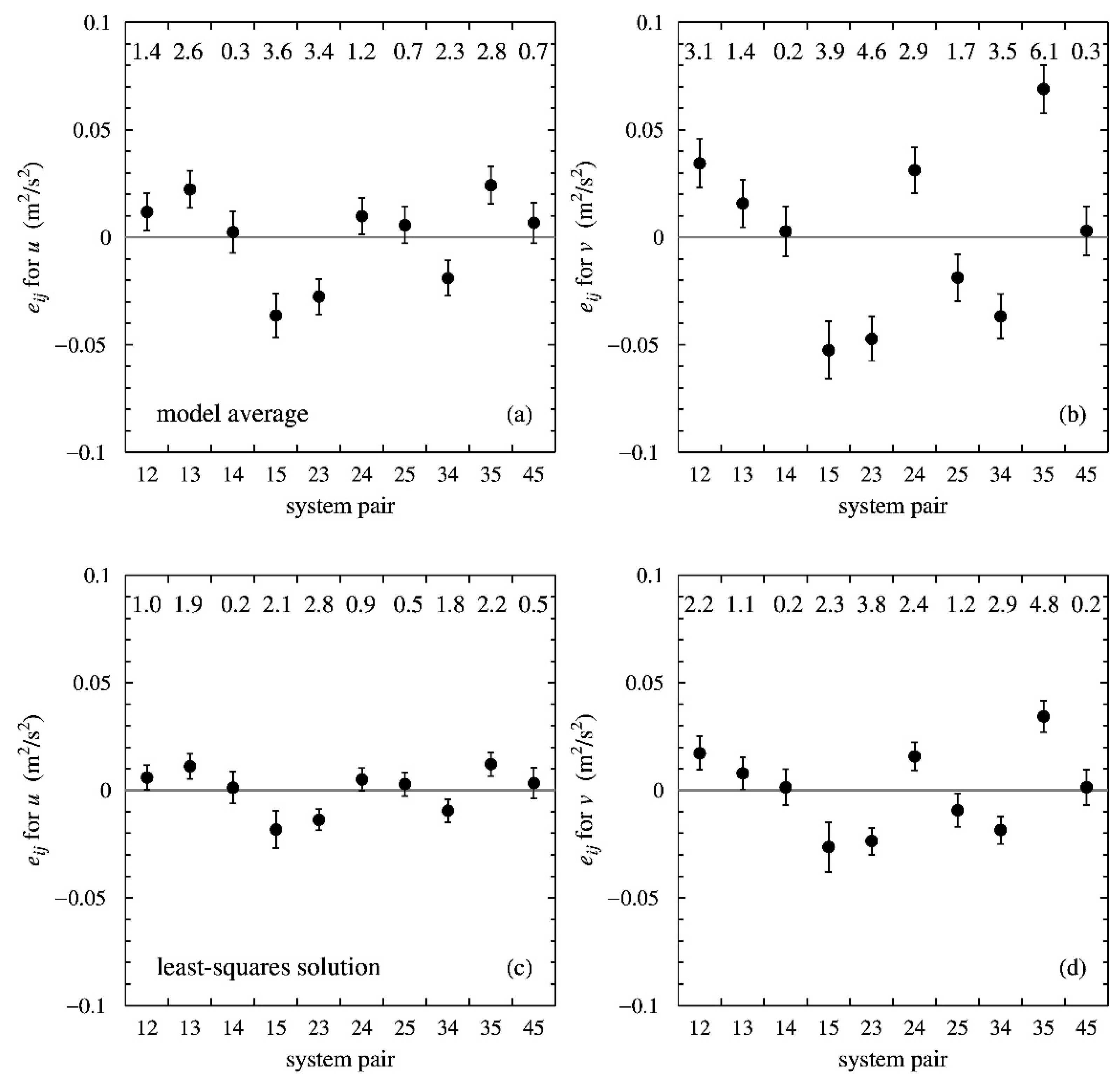
The $n$ error variances ${\sigma }_i^2$ only appear in the $n$ diagonal covariance equations, so these are easily calculated when $a_i$ and $T$ are known. The remaining $n\left(n-1\right)/2$ off-diagonal covariance equations only contain the $n$ essential variables $a_i$ and $T$ ($a_1=1$ because system 1 is the calibration reference) plus the error covariances $e_{ij}$. For quadruple collocations, the authors take all possible sets of $n$ off-diagonal covariance equations, neglect the error covariances in these so the equations take the form $C_{ij}=a_i{a}_{j}T$, and solve each set analytically for $a_i$ and $T$ [3]. There are 15 possible sets, further referred to as models, of which 12 have a solution. Three models cannot be solved, and such models will be referred to as unsolvable. Besides the essential unknowns, each solvable model also yields two error covariances from the remaining two covariance equations that were not used to solve $a_i$ and $T$. See also Appendix A for an example. The number of models grows rapidly with the number of observing systems, see

Table 1. Number of observing systems, number of equations, number of models, and number of solvable and unsolvable models.

Observing Systems	Off-Diagonal Equations	Models	Solvable	Unsolvable
3	3	1	1	0
4	6	15	12	3
5	10	252	162	90
6	15	5005	2530	2475
7	21	116,280	45,615	70,665
8	28	3,108,105	937,440	2,170,665
9	36	94,143,280	21,685,132	72,458,148

. For quintuple collocation there are already 252 models, and analytical solution is practically impossible.

Taking a closer look at the covariance equations with the error covariances neglected, one sees that the unknowns $a_i$ and $T$ appear as a product on one side and the coefficients $C_{ij}$, calculated from the data, on the other. By taking logarithms on both sides, the unknowns are separated and the equations reduce to an ordinary system of linear equations. Suppose a model has been defined by a selection of $n$ off-diagonal covariance equations $\left\{C_{ij}^{\left(m\right)}=a_i{a}_{j}T\right\}$ in which the error covariances are neglected, with $j>i$ and labeled with index $m=1, \dots , n$. Setting $z_1=\log T$, $z_m=\log a_m$ for $m=2,\dots ,n$, and $d_m=\log C_{ij}^{\left(m\right)}$, the off-diagonal covariances read in matrix-vector notation

$$Dz=d$$

(5)

where the matrix $D$ has for each row the value 1 in the first column, $D_{m1}=1$, and one or two additional values 1 in the remaining columns, $D_{mi}=1$ if $i>1$, and $D_{mj}=1$. All other elements of $D$ are zero. The determinant of $D$ can thus only take integer values; the zero-value indicating that system (5) has no solution. See Appendix A for an example.

It may seem awkward to take logarithms, but (5) yields the same solution as the original set of equations $\left\{C_{ij}^{\left(m\right)}=a_i{a}_{j}T\right\}$ as long as all variables are positive. This is certainly the case here. The calibration scalings $a_m$ are generally close to 1, so their logarithms are around 0, and the observed covariances $C_{ij}$ are nonnegative; also when representativeness errors are taken into account (see further down). The common variance $T$ is of the same order of magnitude as the $C_{ij}$. Therefore, problem (5) is well-posed and can be solved numerically with standard methods.

In this work, the inverse of $D$ is calculated using Gaussian elimination, and the solution reads $z=D^{-1}d$. This has the advantage that the analytical solution can be reconstructed, since in components

$$z_m={{\displaystyle \sum }}_{l=1}^n{D}_{ml}^{-1}{d}_l$$

(6)

which implies that after exponentiating

$$T={{\displaystyle \prod }}_{l=1}^n{\left(C_{ij}^{\left(l\right)}\right)}^{D_{1l}^{-1}}$$

(7)

$$a_m={{\displaystyle \prod }}_{l=1}^n{\left(C_{ij}^{\left(l\right)}\right)}^{D_{ml}^{-1}},m>1$$

(8)

so the analytical solutions for the common variance $T$ and the calibration scalings $a_m$ are products of observed covariances raised to a power determined by the components of $D^{-1}$. The error variances are given by ${\sigma }_m^2=C_{mm}-a_m^{2}T$, and from (7) and (8), it follows that

$${\sigma }_1^2=C_{11}-{{\displaystyle \prod }}_{l=1}^n{\left(C_{ij}^{\left(l\right)}\right)}^{D_{1l}^{-1}}$$

(9)

$${\sigma }_m^2=C_{mm}-{{\displaystyle \prod }}_{l=1}^n{\left(C_{ij}^{\left(l\right)}\right)}^{D_{1l}^{-1}+2D_{ml}^{-1}},m>1$$

(10)

Note that in (10), factors may cancel in the exponent.

The same logarithmic transformation can also be applied to all off-diagonal covariance equations and solved with the least-squares method, having the advantage that the solution is given directly in the logarithms of the basic unknowns rather than combinations of them. If the number of equations permits, error covariances can be included by adding extra variables $z_m=\log \left(T+e_{ij}\right)$ with $m>n$.

The determinant of $D^{\mathrm{T}}D$ in the least-squares solution equals the number of soluble models for quadruple and quintuple collocations. In the determined cases, matrices $D^{-1}$ have only integer elements, see Appendix A; in the overdetermined case, the Moore–Penrose pseudoinverse ${\left(D^{\mathrm{T}}D\right)}^{-1}{D}^{\mathrm{T}}$ also contains rational numbers. In Appendix B, it is shown that the least-squares solution is the geometric mean of all model solutions, a consequence of the fact that in logarithmic space the overdetermined solution is the arithmetic average of the determined ones.

A solution method equivalent to the least-squares solution is minimizing a quadratic cost function $J$ defined as

$$J={{\displaystyle \sum }}_{i=1}^n{{\displaystyle \sum }}_{j=i+1}^n{\left(a_i{a}_{j}T-C_{ij}\right)}^2$$

(11)

to $a_i$ and $T$ using a standard conjugate-gradient method.

3.3. Iterative Solution

The covariance equations for each possible model are solved in an iterative scheme that starts with assuming that the data are already perfectly calibrated, so $a_i^{\left(0\right)}=1$ and $b_i^{\left(I\right)}=0$, $i=1, 2, \dots , n$, where the superscript $I$ stands for the iteration index. The relation between the calibrated measured values in iteration $I$, $y_i^{\left(I\right)}$, and the original values, $x_i$, is

$$y_i^{\left(I\right)}=\frac{x_i-b_i^{\left(I\right)}}{a_i^{\left(I\right)}}$$

(12)

In each iteration, the averages and covariances are recalculated from the calibrated data and the covariance equations are solved, but now the solution does not yield the calibration coefficients $a_i$ and $b_i$ themselves, but their updates $\Delta a_i$ and $\Delta b_i$. Of course, $\Delta b_1=0$ and $\Delta a_1=1$ because system 1 is chosen as calibration reference. The calibration coefficients are updated as

$$b_i^{\left(I\right)}=b_i^{\left(I-1\right)}+\Delta b_i,a_i^{\left(I\right)}=a_i^{\left(I-1\right)}\Delta a_i,i=2, 3,\dots , n$$

(13)

Iteration has converged when $\left|\Delta b_i\right|<\epsilon$ and $\left|1-\Delta a_i\right|<\epsilon$, with $\epsilon ={10}^{-6}$. This usually takes about ten steps.

This iteration scheme has two advantages. First, in each iteration, the standard deviation of the difference between each pair of calibrated measurements, ${\sigma }_{ij}^{\left(I\right)}$, can be calculated, and this can be used in the next iteration to detect (and exclude) outliers. The iteration starts with a large value ${\sigma }_{ij}^{\left(0\right)}=3$ m²s⁻², and collocations are excluded whenever

$$\left|y_i^{\left(I\right)}-y_j^{\left(I\right)}\right|>4{\sigma }_{ij}^{\left(I-1\right)}$$

(14)

(hence the name “4-sigma test”).

Second, it allows for proper inclusion of representativeness errors calculated as differences in spatial variances of the uncalibrated data. Suppose the observation systems are sorted to decreasing spatial resolution and that $r_l^2$ is the representativeness error of higher resolution system $l$ with respect to lower resolution system $l+1$. As shown in [3], the (calibrated) representativeness errors can be incorporated in the observed covariances by the substitution

$$C_{ij}\to C_{ij}-{{\displaystyle \sum }}_{l=max\left(i,j\right)}^{n-1}{r}_l^2$$

(15)

In other words, the known representativeness errors are put to the other side of the covariance Equation (3) together with the known covariances $C_{ij}$. Error covariances that are known a priori can be incorporated in this way.

3.4. Representativeness Errors

In general, the representativeness errors cannot be retrieved from the error covariances. The number of off-diagonal covariance equations is $n_{od}=n\left(n-1\right)/2$, so the number of error covariances that can be retrieved is $n_{ec}=n_{od}-n=n\left(n-3\right)/2$. The number of representativeness errors is $n_{re}=\left(n-1\right)\left(n-2\right)/2=n_{ec}+1$, so there is always one off-diagonal covariance equation lacking. This can be circumvented when the two coarsest resolution systems have the same spatial and temporal resolution. In the case considered here, one could try ECMWF forecasts with different analysis times. However, as already remarked in [3], this would introduce an additional error covariance between the two forecasts, and the resulting model has no solution.

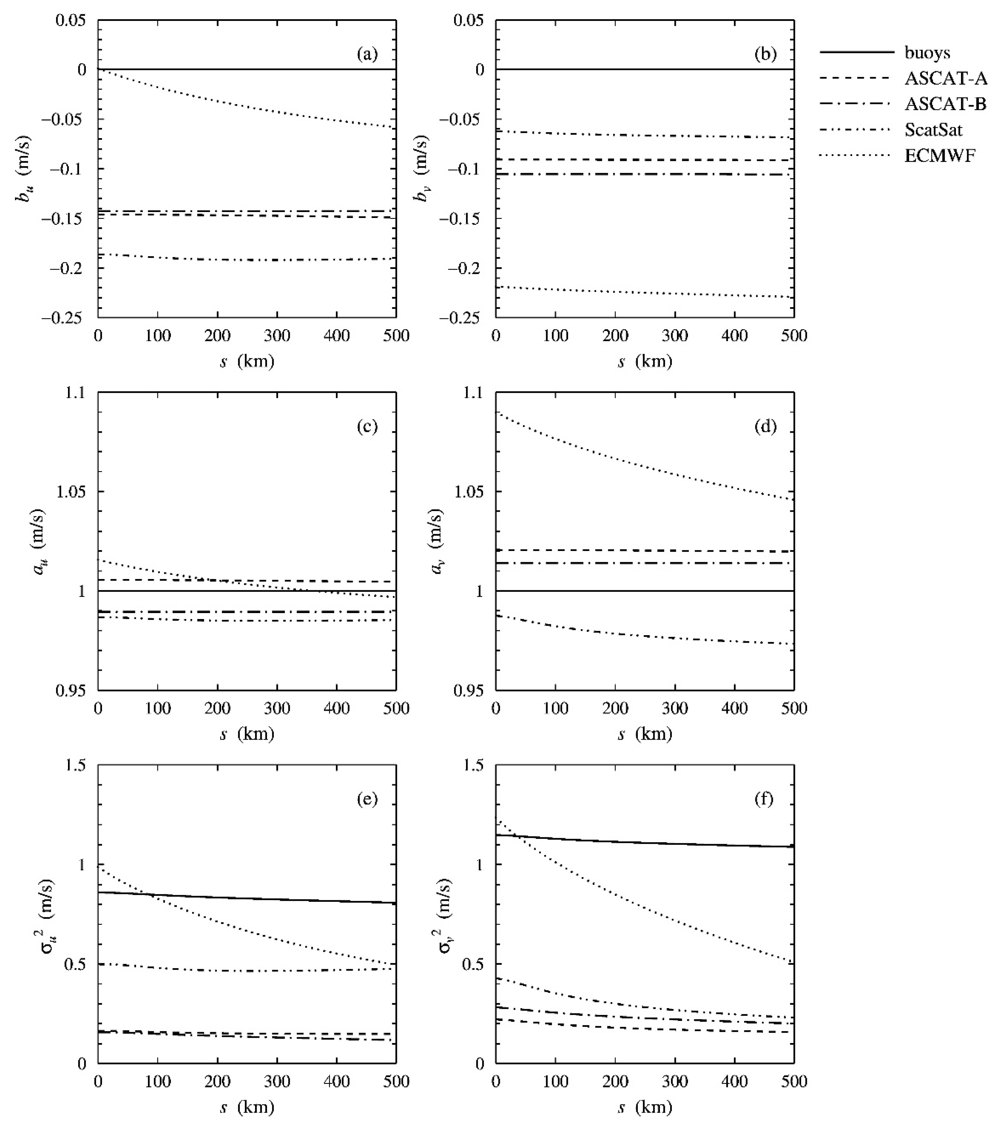
As a consequence, the representativeness errors must be estimated in a different way. In this study, they are obtained from differences in spatial variance as a function of sample length (further referred to as scale) [13]. Figure 1 shows the difference in spatial variance $\Delta V\left(s\right)=V_{scat}\left(s\right)-V_{ECMWF}\left(s\right)$, as a function of scale $s$ for ASCAT-B, ASCAT-A, and ScatSat. Figure 1 is the same as Figure 2 in [3]. In the terminology of Equation (15), the ScatSat representativeness error with respect to the ECMWF model, $r_4^2$, is defined as $r_4^2=V_{ScatSat}\left(s\right)-V_{ECMWF}\left(s\right)$, the height of the dotted curve. The representativeness error $r_3^2$ of ASCAT-A relative to ScatSat equals the vertical distance between the dotted curve and the solid curve, and that of ASCAT-B relative to ASCAT-A, $r_2^2$, by the vertical distance between the dashed and the solid curve. The representativeness error of ASCAT-B relative to the ECMWF background equals $r_2^2+r_3^2+r_4^2$, the height of the dashed curve, in Figure 1. The representativeness errors increase with scale.

Previous work indicated that the optimum scale for calculating the representativeness errors is about 200 km for the zonal wind component $u$ and about 100 km for the meridional wind component $v$. Both correspond to a spatial representativeness wind vector component variance of about 0.3 m² s⁻² for the ASCATs.

Note that the spatial variances $V_{scat}$ and $V_{ECMWF}$ should be divided by the square of the calibration scaling before calculating the representativeness errors and applying (15) in order not to mix up calibrated and uncalibrated quantities when applying the iterative scheme presented in Section 3.3. Note also that the curves for ASCAT-A and ASCAT-B are not identical. This is due to the time difference of about 50 min in the local overpass time between the two sensors, mainly due to a different orbit phase. They, therefore, sample different weather at a particular phase of the diurnal cycle (both sensors are in a mid-morning sun-synchronous orbit). When mesoscale turbulent processes play a role, ASCAT-A and ASCAT-B can give quite different wind fields [18].

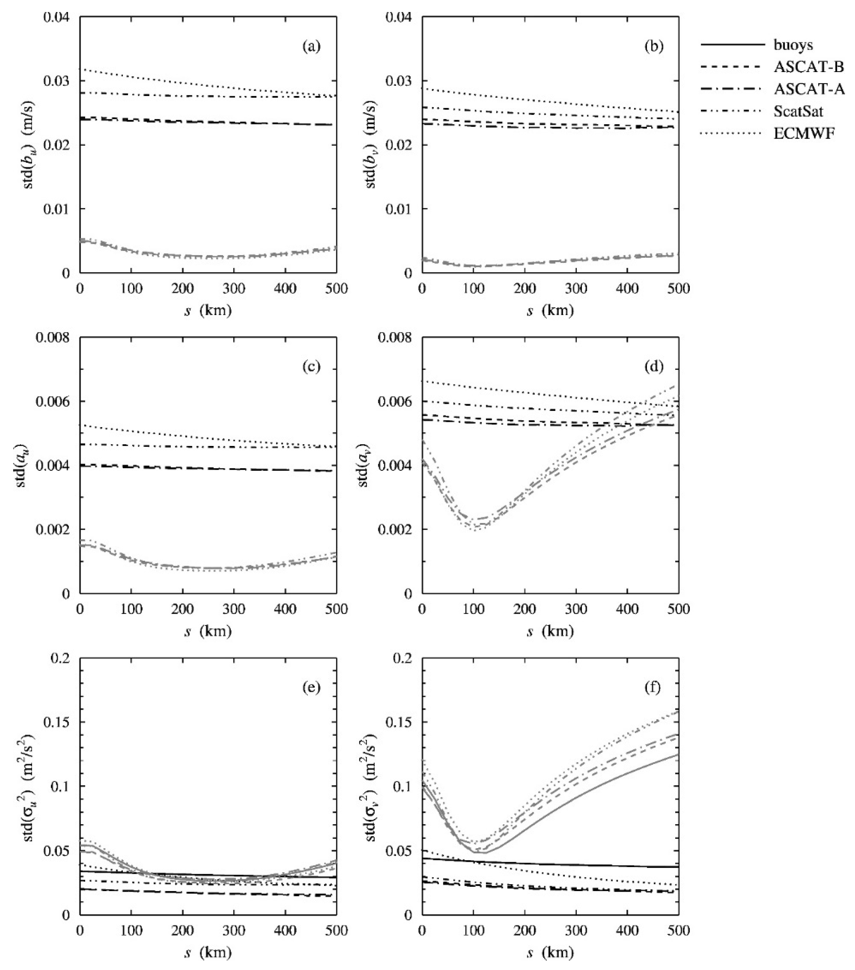
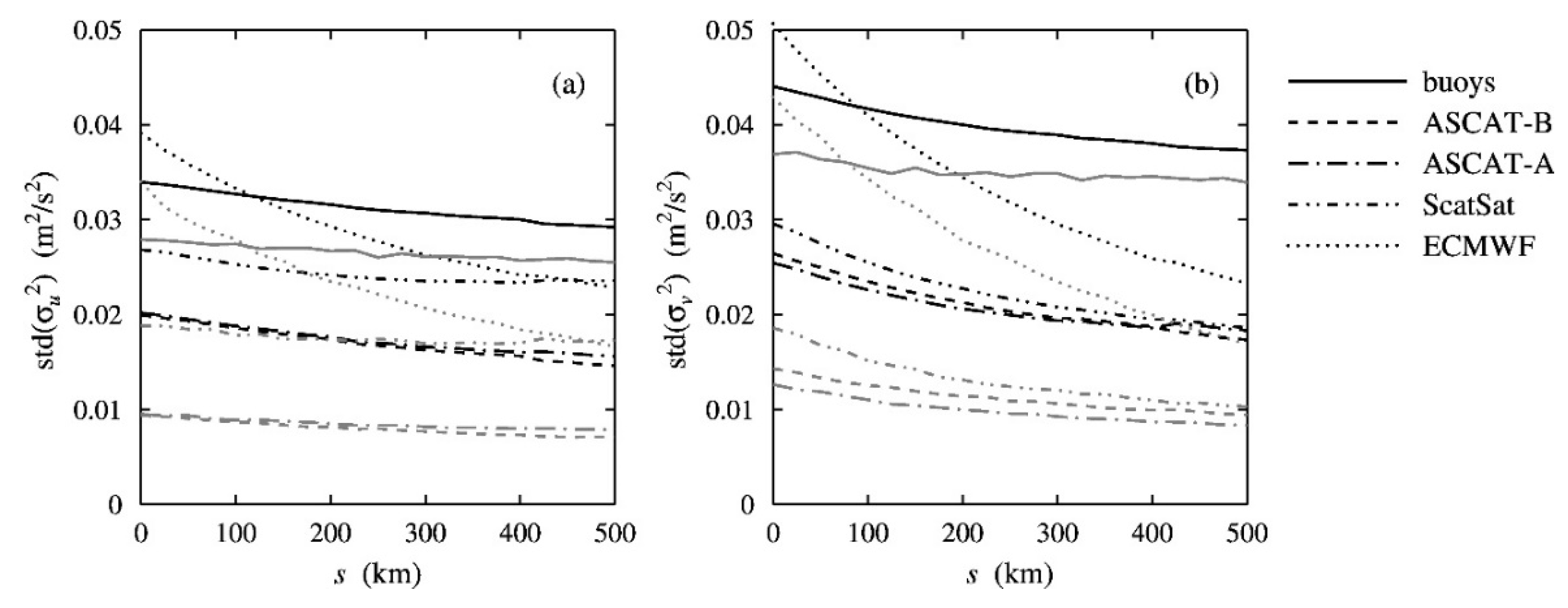
3.5. Precision Estimate

The primary source of uncertainty is in the wind components $x_i$. The calibration scalings and common variance are functions of the covariances $C_{ij}$ which are second-order statistics. To calculate the precision in the covariances would require fourth-order statistics, but these are very sensitive to outliers and give no usable results for data sets with the size considered here. Therefore, a different approach is followed in this work.

The first step is to run a quintuple collocation analysis on the original data to calculate calibration coefficients and the error variances. Then, the reference system is adopted as common signal $t$ and a synthetic data set is constructed using (1) with Gaussian random errors. This yields a data set that is not precisely equivalent to the original data set because the observation errors of the reference system are part of the signal, but it is close enough for a good precision estimate. Next, a quintuple collocation analysis is performed on the synthetic data set. The process is repeated a sufficient number of times (10,000 in the cases presented here), and the first and second moments of each variable are updated. Finally, averages and standard deviations are calculated for each model separately. The averages lie close to the values used to construct the synthetic data (no results shown), while the standard deviations give the precision estimates. Finally, the model results are averaged over all models. The same procedure, except for the model averaging, is also followed for the least-squares solution.

4. Results and Discussion

As a check, the numerical solutions, calculated in double precision, were compared to the analytical ones for the quadruple collocations in [3] and were found to agree to at least six decimal places.

4.1. Number of Solvable Models

Table 1 gives the number of observing systems, the number of off-diagonal covariance equations, the number of models, and the number of solvable and unsolvable models obtained from (6). The number of models, $n_m$, satisfies

$$n_m=\left(\begin{array}{c}n\left(n-1\right)/2\\ n\end{array}\right)$$

(16)

with $n$ the number of observing systems. The fraction of solvable models decreases from 80% for quadruple collocation to about 23% for nonuple collocations, but still the number of solvable models increases rapidly.

Table 1 shows that there are 162 solvable models for quintuple collocations. As for quadruple collocations, different models lead to different solutions so it makes little sense to present them all. Therefore, only statistical results will be shown, and the statistics will be better than those from the 12 solvable models in a quadruple collocation analysis. The model-averaged results will also be compared with those of the least-squares solution.

4.2. Calibration Coefficients and Error Standard Deviations

Figure 2a,b show the results for the calibration biases, Figure 2c,d for the calibration scalings, and Figure 2e,f for the error variances. Figure 2a,c,e show results for the zonal wind component $u$ and Figure 2b,d,f for the meridional wind component $v$, all against the scale $s$ at which the representativeness errors are calculated. The curves give the averages over all 162 model solutions. The calibration coefficients are given for the forward calibration transformation, $x_i^{cal}=\left(x_i-b_i\right)/a_i$ with $x_i$ the raw data of system $i$ and $x_i^{cal}$ the calibrated data.

Figure 2 shows that the results depend rather weakly on $s$. The strongest dependency on the representativeness error is found for the ECMWF background at both $u$ and $v$, and, to a lesser extent, for the ScatSat error variance at $v$. This agrees with earlier triple and quadruple collocation analyses for these systems.

The model averages in Figure 2 are the same as the least-squares solution to at least three decimal places. In Appendix B, it is shown that the least-squares solution equals the geometric mean of all model solutions.

4.3. Statistical Accuracy and Model Spread

Figure 3 shows the results for the accuracy, i.e., the standard deviation (std) of the solutions of all 10,000 synthetic data sets averaged over all models, and the model spread, i.e., the standard deviation of all model solutions. The accuracy is almost the same for each separate model so its average over all models is representative. The black curves in Figure 3 give the accuracy; the gray ones, the model spread. The accuracy depends weakly on the representativeness errors, while the model spread shows much stronger dependency, especially for $v$, similar to the quadruple collocation results in [3]. For the calibration biases, Figure 3a,b, the model spread is much smaller than the accuracy. For the calibration scalings, Figure 3c,d, the model spread is smaller than the accuracy except for $v$ at large scales. For the observation error variances, Figure 3e,f, the model spread in ${\sigma }_u^2$ is larger than the accuracy, but the two are about equal at $s$ between 200 km and 300 km. The spread in ${\sigma }_v^2$ shows a sharp minimum for $v$ at $s\approx 100$ km, like for quadruple collocation analysis on the same data.

For the buoys and the ECMWF model, the spread at the minimum is about equal to the accuracy, but for the scatterometers, it is twice as high. The results in Figure 3e,f for the observation error variances show that only with proper values of the representativeness errors, the model spread and the estimated statistical noise are close together, indicating optimal—but not perfect—model consistency.

Figure 4 shows the accuracies of the model average (black curves) and of the least-squares solution (gray curves) for the observation error variances. For the calibration coefficients, the accuracy of the least-squares solution is the same as that of the model average (no results shown), but for the observation error variances, it is smaller.

Note that the observation error variances are more accurate than one would expect from simple arguments. They are obtained from (3) as

$${\sigma }_i^2=\frac{C_{ii}}{a_i^2}-T$$

(17)

Both terms on the right-hand side of Equation (17) are a quotient of an odd number of covariances $C_{ij}$ with one covariance more in the numerator than in the denominator. The common variance $T$ is about 26 m²s⁻² for $u$ and about 18 m²s⁻² for $v$. Its accuracy is about 0.2 m²s⁻² for both $u$ and $v$, and the same accuracy can be expected for the other term. If the terms were not correlated, the accuracy in the error variance would be about 0.4 m²s⁻², but the correlations keep the accuracy down by two orders of magnitude to the values shown in Figure 3. Nevertheless, the observation error variances are obtained as the difference between two large numbers and are, therefore, sensitive to statistical noise. The same applies to the observation error covariances.

4.4. Error Covariances

Figure 5 shows the observation error covariances $e_{ij}$ averaged over all models (a, b) and obtained from the least-squares solution (c, d), with the representativeness errors evaluated at $s=200$ km for $u$ and $s=100$ km for $v$. The model average is, of course, taken only over those error covariances that are a solution of the model under consideration. The dots give the values of the error covariances, while the error flags indicate their statistical accuracy. System 1 stands for the buoys, system 2 for ASCAT-B, system 3 for ASCAT-A, system 4 for ScatSat, and system 5 for the ECMWF forecasts. The numbers along the top of each panel give the absolute value of the error covariance in units of its standard deviation to indicate the statistical significance.

The observation error covariances from the least-squares solution are smaller than those from the model average by a factor of about two. This seems odd because the observation error variances of least-squares solution and model average agree to three decimal places at least. The model average is taken strictly over those five error covariances out of ten that can be solved for each model; the other five covariances were set to zero in order to solve for the calibration scalings and error variance, and do not contribute to the average. The least-squares solution is the geometric mean of the model solutions, but apparently, the error covariances that are set to zero are also included in the average, leading to an underestimation by a factor of two. The same happens for the second moments so the accuracies of the least-squares solution are also underestimated, as can be seen from Figure 5. This makes the least-squares method less-suited for analysis of the error covariances.

There are some observation error covariances that significantly (more than three standard deviations) differ from zero. The first one is $e_{15}$, the error covariance between buoys and ECMWF. It could be possible that buoy measurements in the collocation data set were assimilated in the ECMWF model and wind biases propagate to the ECMWF forecast fields use here. However, that would lead to positive error covariances, while the values for $e_{15}$ in Figure 5 are all negative.

A second nonzero error covariance is $e_{23}$, between ASCAT-A and ASCAT-B. Since the data of both instruments are processed in the same way, deficiencies in the processing chain could lead to error correlations. However, one would expect positive error covariances, while all values of $e_{23}$ in Figure 5 are negative.

The largest and positive error covariances are found for $e_{35}$, between ASCAT-A and ECMWF, in particular for $v$. Abdallah and De Chiara [4] also report error correlations between ASCAT-A and ECMWF, but for wind speed. They attribute this to long-lasting effects of ASCAT-A assimilation in the ECMWF model. However, this effect should then also be observable in $e_{25}$, the error covariance between ASCAT-B and ECMWF, since the ASCAT-B wind fields have similar characteristics as those from ASCAT-A (though differences may occur, as mentioned in Section 3.4). The values of $e_{25}$ in Figure 5 differ not significantly from zero for $u$ and are negative for $v$.

A possible explanation for the results in Figure 5 is offered by the fact that the ECMWF model contains systematic wind direction biases (e.g., [19]). These biases are known for quite some time. They are a tough problem and any attempt so far to solve them led to unacceptable deterioration of the forecast skill at other locations and forecast range. The multiple collocation analysis will treat the model biases as random errors, thus violating the basic assumption that the observation errors are random. Furthermore, systematic errors in the scatterometer winds caused by errors in the processing cannot be fully excluded.

5. Discussion

In [3], the authors posed the question of whether the model spread was due to statistical noise or to inconsistencies in the underlying error model (1). The answer is that both effects play a role. If a synthetic data set without errors is used, all models give the same solution (no results shown), so the model spread is at least partly generated by statistical noise. On the other hand, the results for the observation error variances and covariances show that the underlying error model is not fully consistent, notably for $v$, even with appropriate values for the representativeness errors.

To conclude,

Table 2. Observation error standard deviations and their accuracies.

Observing System	${\mathit{\sigma }}_{\mathit{u}}$	$\mathbf{s}\mathbf{t}\mathbf{d}\left({\mathit{\sigma }}_{\mathit{u}}\right)$	${\mathit{\sigma }}_{\mathit{v}}$	$\mathbf{s}\mathbf{t}\mathbf{d}\left({\mathit{\sigma }}_{\mathit{v}}\right)$
	(m/s)	(m/s)	(m/s)	(m/s)
buoys	0.914	0.017	1.063	0.020
ASCAT-A	0.372	0.022	0.505	0.029
ASCAT-B	0.390	0.025	0.444	0.020
ScatSat	0.683	0.018	0.594	0.021
ECMWF	0.845	0.017	1.006	0.021

gives the results for the observation error standard deviation, $\sigma$, with the estimated statistical accuracy obtained from the model average, $\mathrm{std}\left(\sigma \right)$. The results are with representative errors evaluated at $s=200$ km for $u$ and $s=100$ km for $v$. Because the accuracies are estimated with Gaussian errors, which may be an optimistic assumption, it is wise to treat the accuracies in Table 2 with care. Moreover, the accuracies are given at the one-sigma level, and the collocation data set is but one realization of all possible measurement error configurations.

6. Conclusions

The accuracy and consistency of a quintuple collocation analysis of ocean surface vector winds from buoys, scatterometers, and NWP forecasts is studied. A new solution method for the covariance equations is introduced. By a logarithmic transformation, the covariance equations reduce to an ordinary system of linear equations that is efficiently solved using matrix inversion. There are 252 possible determined subsets of the covariance equations, referred to as models, of which 162 have a solution for the calibration coefficients, the observation error variances, and five additional error covariances. Representativeness errors are included as differences between spatial variances, and the results are presented as a function of the scale at which the representativeness errors are evaluated. The logarithmic transformation can also be applied to all covariance equations, leading to the least-squares solution for the calibration coefficients and the observation error variances. The least-squares solution is the geometric average over all model solutions. It is the same as the average over all model solutions to three decimal places at least, except for the error covariances which are underestimated.

The accuracy is estimated from synthetic data sets constructed by selecting the buoy data as truth, applying the calibration coefficients from the quintuple collocation analysis to construct the other data, and adding random Gaussian errors with standard deviations also from the quintuple collocation analysis. This process is repeated 10,000 times for all models as well as for the least-squares solution. Statistics of all variables are updated so averages and standard deviations of the calibration coefficients and error (co-)variances can be calculated.

The accuracy obtained thus is compared to the spread in the 162 model solutions. For the calibration coefficients, the spread is smaller than the accuracy; for the observation error variances, the spread and the accuracy are about equal, but only when representativeness errors are properly included, in particular, for the meridional wind component $v$. Further, some error covariances differ significantly from zero, indicating that the underlying error model is not fully consistent, even when representativeness errors are included properly. These results cannot be explained by error correlations between various systems, but are more likely caused by systematic errors in the ECMWF model and the scatterometer processing.

The accuracy of the observation error standard deviations is about 0.02 to 0.03 m/s at the one-sigma level for a data set of 2454 collocations. Because the accuracy is estimated from Gaussian errors, which may be too optimistic an assumption, it is wise to treat this value with care.

References

1. Stoffelen, A. Toward the True Near-surface Wind Speed: Error Modelling and Calibration using Triple Collocation. J. Geophys. Res. 1998, 103, 7755–7766. [Google Scholar] [CrossRef]
2. Vogelzang, J.; Stoffelen, A.; Verhoef, A.; Figa-Saldaña, J. On the Quality of High-resolution Scatterometer Winds. J. Geophys. Res. 2011, 116, C10033. [Google Scholar] [CrossRef]
3. Vogelzang, J.; Stoffelen, A. Quadruple Collocation Analysis of In-situ, Scatterometer, and NWP Winds. J. Geophys. Res. Oceans 2021, 126, e2021JC017189. [Google Scholar] [CrossRef]
4. Abdalla, S.; De Chiara, G. Estimating Random Errors of Scatterometer, Altimeter, and Model Wind Speed Data. IEEE JSTARS 2017, 10, 2406–2414. [Google Scholar] [CrossRef]
5. Danielson, R.E.; Johannessen, J.A.; Quartly, G.D.; Rio, M.-H.; Chapron, B.; Collard, F.; Donlon, C. Exploitation of Error Correlation in a Large Analysis Validation: GlobCurrent Case Study. Remote Sens. Environ. 2018, 217, 476–490. [Google Scholar] [CrossRef]
6. Hoareau, N.; Portabella, M.; Lin, W.; Ballabrera-Poy, J.; Turiel, A. Error Characterization of Sea Surface Salinity Products using Triple Collocation Analysis. IEEE Trans. Geosci. Remote Sens. 2018, 56, 5160–5168. [Google Scholar] [CrossRef]
7. Roebeling, R.; Wolters, E.; Meirink, J.; Leijnse, H. Triple Collocation of Summer Precipitation Retrievals from SEVIRI over Europe with Gridded Rain Gauge and Weather Radar Data. J. Hydrometeorol. 2012, 13, 1552–1566. [Google Scholar] [CrossRef]
8. Wild, A.; Chua, Z.-W.; Kuleshov, Y. Triple Collocation Analysis of Satellite Precipitation Estimates over Australia. Remote Sens. 2022, 14, 2724. [Google Scholar] [CrossRef]
9. Gruber, A.; Su, C.-H.; Crow, W.T.; Zwieback, S.; Dorigo, W.A.; Wagner, W. Estimating Error Cross-correlations in Soil Moisture Data Sets using Extended Collocation Analysis. J. Geophys. Res. Atmos. 2016, 121, 1208–1219. [Google Scholar] [CrossRef]
10. Fan, X.; Lu, Y.; Liu, Y.; Li, T.; Xun, S.; Zhao, X. Validation of Multiple Soil Moisture Products over an Intensive Agricultural Region: Overall Accuracy and Diverse Responses to Precipitation and Irrigation Events. Remote Sens. 2022, 14, 3339. [Google Scholar] [CrossRef]
11. Gruber, A.; De Lannoy, G.; Albergel, C.; Al-Yaari, A.; Brocca, L.; Calvet, J.C.; Colliander, A.; Cosh, M.; Crow, W.; Dorigo, W.; et al. Validation Practices for Satellite Soil Moisture Retrievals: What are (the) Errors? Remote Sens. Environ. 2020, 244, 111806. [Google Scholar] [CrossRef]
12. Lin, W.; Portabella, M.; Stoffelen, A.; Vogelzang, J.; Verhoef, A. ASCAT Wind Quality under High Sub-cell Wind Variability Conditions. J. Geophys. Res. Oceans 2015, 120, 5804–5819. [Google Scholar] [CrossRef]
13. Vogelzang, J.; King, G.P.; Stoffelen, A. Spatial Variances of Wind Fields and their Relation to Second-order Structure Functions and Spectra. J. Geophys. Res. Oceans 2015, 120, 1048–1064. [Google Scholar] [CrossRef]
14. Su, C.H.; Ryu, D.; Crow, W.T.; Western, A.W. Beyond Triple Collocation: Applications to Soil Moisture Monitoring. J. Geophys. Res. Atmos. 2014, 119, 6419–6439. [Google Scholar] [CrossRef]
15. Crow, W.T.; Su, C.-H.; Ryu, D.; Yilmaz, M.T. Optimal Averaging of Soil Moisture Predictions from Ensemble Land Surface Model Simulations. Water Resour. Res. 2015, 51, 9273–9289. [Google Scholar] [CrossRef]
16. McColl, K.A.; Vogelzang, J.; Konings, A.G.; Entekhabi, D.; Piles, M.; Stoffelen, A. Extended Triple Collocation: Estimating Errors and Correlation Coefficients with Respect to an Unknown Target. Geophys. Res. Lett. 2014, 41, 6229–6236. [Google Scholar] [CrossRef]
17. Pierdicca, N.; Fascetti, F.; Pulvirenti, L.; Crapolicchio, R.; Munoz-Sabater, J. Quadruple Collocation Analysis for Soil Moisture Product Assessment. IEEE Geosci. Remote Sens. Lett. 2015, 12, 1595–1599. [Google Scholar] [CrossRef]
18. King, G.P.; Portabella, M.; Lin, W.; Stoffelen, A. Correlating Extremes in Wind Divergence with Extremes in Rain over the Tropical Atlantic. Remote Sens. 2022, 14, 1147. [Google Scholar] [CrossRef]
19. Belmonte Rivas, M.; Stoffelen, A. Characterizing ERA-Interim and ERA5 Surface Wind Biases using ASCAT. Ocean Sci. 2019, 15, 831–852. [Google Scholar] [CrossRef] [Green Version]
Figure 1. Difference between the spatial variance of ASCAT-A, ASCAT-B, and ScatSat and that of ECMWF, Δ V ( s ) , as a function of s for the zonal wind component u (a) and for the meridional wind component v (b).
Remotesensing 14 04552 g001
Figure 2. Quintuple collocation results as a function of the scale at which the representativeness errors are calculated for the calibration biases for u (a), the calibration biases for v (b), the calibration scalings for u (c), the calibration scalings for v (d), the error variances for u (e), and the error variances for v (f), all averaged over all models.
Remotesensing 14 04552 g002
Figure 3. Quintuple collocation results for the accuracy (black curves) and the model spread (gray curves) as a function of the scale at which the representativeness errors are evaluated for the calibration biases for u (a), the calibration biases for v (b), the calibration scalings for u (c), the calibration scalings for v (d), the error variances for u (e), and the error variances for v (f).
Remotesensing 14 04552 g003
Figure 4. Accuracy of the model average (black curves) and the least-squares solution (gray curves) for the observation error variances in u (a) and those in v (b).
Remotesensing 14 04552 g004
Figure 5. Error covariances and their accuracies from the model average for u (a), the model average for v (b), the least-squares solution for u (c), and the least-squares solution for v (d).
Remotesensing 14 04552 g005