Abstract
The melt pond fraction (MPF) is an important geophysical parameter of climate and the surface energy budget, and many MPF datasets have been generated from satellite observations. However, the reliability of these datasets suffers from short temporal spans and data gaps. To improve the temporal span and spatiotemporal continuity, we generated a long-term spatiotemporally continuous MPF dataset for Arctic sea ice, which is called the Northeast Normal University-melt pond fraction (NENU-MPF), from Moderate Resolution Imaging Spectroradiometer (MODIS) data. First, the non-linear relationship between the MODIS reflectance/geometries and the MPF was constructed using a genetic algorithm optimized back-propagation neural network (GA-BPNN) model. Then, the data gaps were filled and smoothed using a statistical-based temporal filter. The results show that the GA-BPNN model can provide accurate estimations of the MPF (R2 = 0.76, root mean square error (RMSE) = 0.05) and that the data gaps can be efficiently filled by the statistical-based temporal filter (RMSE = 0.047; bias = −0.022). The newly generated NENU-MPF dataset is consistent with the validation data and with published MPF datasets. Moreover, it has a longer temporal span and is much more spatiotemporally continuous; thus, it improves our knowledge of the long-term dynamics of the MPF over Arctic sea ice surfaces.
1. Introduction
The melt pond fraction (MPF) of Arctic sea ice is an important geophysical parameter for the climate and surface energy budget of the cryosphere [1,2,3,4], and it has been widely used in sea ice evolution and general circulation models (GCMs) [5,6]. During the summer in the Arctic, melt ponds appear when the snow and/or sea ice on the top of sea ice surface melt [7,8]. These ponds can achieve coverage of up to 50–60% over the entire Arctic sea ice zone [9,10,11,12,13], and up to 75% coverage of first-year ice surfaces [6,11,14].
The formation and disappearance of melt ponds are closely related to changes in the sea ice albedo [10,15,16], and the expansion of melt ponds during summer can significantly decrease the surface albedo of Arctic sea ice [17]. This decrease in the surface albedo can lead to more absorption of solar radiation, which can further amplify the climate change in the Arctic via the sea-ice feedback mechanism [18]. It has also been reported that the MPF is considered to be a good predictor for the Arctic sea ice extent in September and can be used to improve forecasts of seasonal sea ice changes and climate models [19,20,21,22,23].
Therefore, it is crucial to monitor the spatiotemporal dynamics and evolution of the MPF over the Arctic sea ice surface. In recent decades, the MPF of Arctic sea ice has typically been measured through ship-based visual observations, aerial photography, and satellite remote sensing [24,25,26,27,28,29,30]. However, owing to the limited spatial coverage of surface measurements, the spatiotemporal variations in the MPF cannot be represented well by ground measurements [24,31,32,33,34], such as the data collected by floating buoys [31], fixed ice stations [33], and cruise ships [34,35].
Therefore, high-spatial-resolution images obtained from tethered balloons [25], unmanned aerial vehicles (UAVs) [36], helicopters [28,37], planes [38], and satellite platforms [26,39,40,41,42,43] are more commonly used to derive the MPF of Arctic sea ice. The various classification methods were developed to estimate the MPF of Arctic sea ice based on various types of high-spatial-resolution images, e.g., aerial photographs [37,44,45], Landsat [39,46], Sentinel-2 [43], QuickBird [42], and WorldView-2 [37,41] data.
However, owing to their limited spatial coverage and relatively long revisit cycles, these high-spatial-resolution data cannot well represent the spatiotemporal variations in the MPF over the entire Arctic sea ice area [38,40,45,47,48,49]. Therefore, moderate-spatial-resolution satellite data with much more frequent observations, such as Moderate Resolution Imaging Spectroradiometer (MODIS) and Medium Spectral Resolution Imaging Spectrometer (MERIS) data, are usually considered to be more suitable for generating long-term MPF datasets for Arctic sea ice [50,51,52,53].
Recently, many MPF datasets have been generated from data obtained by multiple remote sensing platforms and sensors. Tschudi et al. [50] proposed a linear spectral unmixing method to derive the fractional coverages of different surface types (e.g., white ice, snow-covered ice, melt ponds, and open ocean water) from MODIS data, and their results revealed that the estimated MPF in the Beaufort/Chukchi Sea region during the summer of 2004 is in good agreement with the measurements acquired by aerosonde unpiloted aerial vehicles and a surface campaign.
To reduce the computation cost of the linear spectral unmixing method, an artificial neural network method was used to speed up the procedure for estimating the MPF [54], and a MPF dataset over the Arctic sea ice surface from 2000 to 2011 was derived by researchers at the University of Hamburg (hereinafter referred to as the UH-MPF dataset) [55]. Although the linear spectral unmixing method can be used to estimate the MPF, it results in large estimation uncertainty due to the prior fixed spectral reflectance of the sea ice components, especially when the MPF and melt pond depth change significantly [56].
To overcome this issue, Zege et al. [56] proposed a melt pond detector (MPD) algorithm to retrieve the MPF of Arctic sea ice from MERIS data. An asymptotic radiative transfer theory (AART) model [4,57,58] was developed to simulate the bidirectional reflectance factor (BRF), black-sky, and white-sky albedo over the surfaces of snow, white ice, and melt ponds. Then, the MPF and albedo over the Arctic region were accurately retrieved from the MERIS data using an iterative procedure.
Finally, a daily MPF dataset for Arctic sea ice from 2002 to 2011 was generated from MERIS Level 1B data by researchers at the University of Bremen (hereinafter referred to as the UB-MPF dataset) [51,52,59]. As MERIS data were not obtained after 2011, the researchers at the University of Bremen also used the data acquired by the Ocean and Land Color Instrument (OLCI) onboard Sentinel-3 to generate an MPF dataset for Arctic sea ice (hereinafter referred to as the UB-OLCI dataset) from 2017 to the present based on a procedure similar to the MPD [60].
In addition, the MPF can also be estimated by establishing the relationship between the satellite observations and MPF data collected from multiple sources. Ding et al. [22] proposed an ensemble-based deep neural network method for estimating the MPF and released a long-term MPF dataset for Arctic sea ice from 2000 to 2019 (as it was derived by researchers at Beijing Normal University; it is hereinafter referred to as the BNU-MPF dataset).
Although many MPF datasets for Arctic sea ice have been generated from a variety of satellite observations, the temporal span and spatiotemporal continuity of these datasets still need to be improved. Among these datasets, the UB-MPF dataset was considered to have a higher estimation accuracy because it was derived using a physical-based model [51,56]. However, owing to its relatively short temporal span (2002–2011), the UB-MPF dataset is not suitable for analyzing the long-term trends and evolutions of the MPF. In addition, most of these MPF datasets are spatiotemporally discontinuous due to cloud obscuration, and the analysis results based on the datasets with numerous data gaps are also questionable.
To extend the temporal span and improve spatiotemporal continuity of the MPF datasets, we generated a long-term spatiotemporally continuous MPF dataset for Arctic sea ice from 2000 to 2020, which is called the Northeast Normal University-melt pond fraction (hereinafter referred to as the NENU-MPF) dataset, using an artificial neural network and a statistical-based temporal filter. In the following sections of this article, we present the data and methodologies used in this study in Section 2. We describe the validation and compare the results with satellite-based and ship-based measurements as well as the published MPF datasets in Section 3. We provide a short summary of this study in Section 4.
2. Materials and Methods
2.1. Data
2.1.1. MODIS Daily Surface Reflectance Data
In this study, we used the MODIS Terra daily surface reflectance product (MOD09GA, Version 6) to generate an MPF dataset for Arctic sea ice from 2000 to 2020. The MOD09GA data provide daily atmospheric corrected surface reflectance data for MODIS bands 1–7 (the central wavelengths of bands 1–7 are 648, 859, 466, 554, 1244, 1631, and 2119 nm, respectively), ancillary incident/viewing geometries (e.g., the solar zenith angle (SZA), view zenith angle (VZA), solar azimuth angle (SAA), view azimuth angle (VAA)), and quality control (QC) information with spatial resolutions of 500 m and 1 km. The MOD09GA data over the Arctic region from 2000 to 2020 were downloaded from the Earthdata website (https://www.earthdata.nasa.gov, accessed on 1 October 2021).
Then, the pixels covered with clouds and open ocean water were screened out based the QC information and sea ice concentration data, and only the cloud-free surface reflectance data over the Arctic sea ice zone were retained. Finally, the surface reflectance data were further reprojected from the sinusoidal projection to the polar stereographic projection and were aggregated to a spatial resolution of 12.5 km. In the subsequent training and prediction processes, only the cloud-free surface reflectance data over the Arctic sea ice zone from 8 May to 24 September of each year were employed.
2.1.2. MPF Data
We used the currently available MPF datasets as the training data for the neural network model and as intercomparison data (Table 1). The UB-MPF dataset for 2003 was used as training data for the artificial neural network; and the UB-MPF datasets for other years (from 2004 to 2011), the UB-OLCI dataset, the UH-MPF dataset, and the BNU-MPF dataset were used for comparison with our results. In this study, all of the MPF datasets were reprojected to the polar stereographic projection with a spatial resolution of 12.5 km for comparison. In the comparison, the NENU-MPF dataset was directly compared with the UB-MPF and UB-OLCI datasets; however, it was aggregated to an 8-day composite temporal resolution for comparison with the UH-MPF and BNU-MPF datasets first.

Table 1.
MPF datasets for Arctic sea ice derived from satellite observations.
2.1.3. Validation Data
We used two satellite-based and three ship-based MPF measurements to validate our results, and the spatial distributions of these measurements are shown in Figure 1. The Arctic sea ice melt pond statistics and maps (ASIMPSM) dataset was obtained from high-spatial-resolution (1 m) satellite images using the maximum likelihood supervised classification method [62]. The ASIMPSM datasets were collected in the Beaufort Sea, East Siberian Sea, Canadian Arctic, and Fram Strait during 1999–2001, with scene sizes of 3 to 10 km.
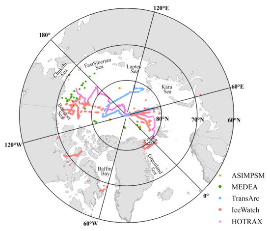
Figure 1.
Spatial distributions of the validation datasets used in this study.
The measurements of Earth data for environmental analysis (MEDEA) dataset was obtained from high-spatial-resolution (1 m) satellite images based on the supervised classification method [63]. The MEDEA dataset was collected at 69–86°N during 1999–2014 for sea ice model validation, with scene sizes of 5 to 25 km. In this study, the original images of the ASIMPSM and MEDEA were aggregated to 12.5 km for comparison with our results.
The IceWatch dataset was compiled from archival visual sea ice observations made by ships in the Northern Hemisphere. The Arctic Shipboard Sea Ice Standardization Tool (ASSIST) was used to document the sea ice conditions (e.g., the ice type, sea ice concentration, snow depth, MPF, and melt pond depth). In this study, the observations collected at 69–89°N in July to August 2011, July 2017, and September 2020 were employed for validation.
The Trans-Arctic survey of the Arctic Ocean in transition (TransArc) dataset was derived from hourly visual observations of sea ice conditions (e.g., sea ice type, sea ice thickness, sea ice concentration, and MPF) acquired by the Polarstern icebreaker from August to September 2011 [34]. The Healy Oden Trans-Arctic Expedition (HOTRAX) dataset was compiled from measurements of ice station, ship, and helicopter aerial images acquired every two hours [9]. In this study, the HOTRAX data acquired at 69.55–89.98°N from August to September 2005 was used for validation.
2.2. Methods
In this study, a genetic algorithm optimized back-propagation neural network (GA-BPNN) and a statistical-based temporal filter were used to generate the NENU-MPF dataset. The main workflow for generating the NENU-MPF dataset is shown in Figure 2.
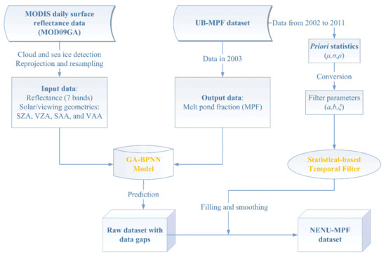
Figure 2.
Workflow for generating the long-term spatiotemporally continuous NENU-MPF dataset.
2.2.1. GA-BPNN Model
In this framework, the GA-BPNN model was used to determine the non-linear relationship between the MODIS directional reflectance/geometries and the MPF derived from the MERIS data (UB-MPF dataset). The daily UB-MPF dataset from May to September 2003 and the corresponding MODIS surface reflectance data were used in the GA-BPNN model, and 70%, 15%, and 15% of the pixels were used as training, validating, and testing data, respectively. The input variables were the surface directional reflectance of the seven MODIS bands and four incident/viewing geometries (SZA, VZA, SAA, and VAA).
The objective output variable was the MPF of the Arctic sea ice. It has been widely reported that the snow, melt ponds, and ocean water are non-Lambertian, and the directional surface reflectance of Arctic sea ice varied significantly with the incident/viewing geometries [4,64]. To capture the reflectance anisotropic properties, the incident/viewing geometries were used as input variables for establishing the relationship between surface reflectance and shortwave surface albedo of Arctic sea ice using an ensemble back-propagation neural network [65].
In this study, a similar approach was carried out for predicting the MPF of Arctic sea ice, and the incident/viewing geometries were also used as input variables. The framework and structure of the GA-BPNN model are shown in Figure 3. As the relationship between the directional surface reflectance/geometries and MPF varied during the different stages of sea ice melting, five GA-BPNN models were separately constructed for each month (from May to September) in this study.
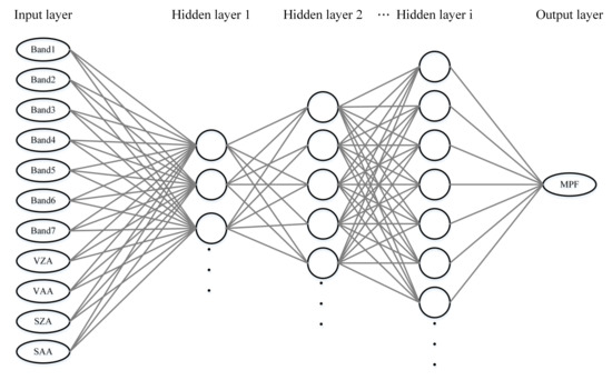
Figure 3.
Framework for estimating the MPF using a GA-BPNN model.
To obtain the optimal structure of the artificial neural network, the following experiments were conducted to determine the structure of the GA-BPNN model. First, the number of hidden layers was assumed to be one, and the influence of the total number of neurons on the prediction accuracy was analyzed. To minimize the influence of the initial values of the weights, we ran the BP neural network model 100 times using random weights and biases assigned for each epoch. Then, the maximum number of hidden layers was assumed to be six, and the influence of the neural network’s structure on the prediction accuracy was examined.
The results of the experiment show that the minimum value of the median root mean square error (RMSE) occurred when the total number of neurons was 22 (the neural network model for May; Figure 4). When the total number of neurons was 22, 20 hidden layer structures could be obtained: (22), (11, 11), (6, 6, 10), (6, 10, 6), (10, 6, 6), (5, 5, 5, 7), (5, 5, 7, 5), (5, 7, 5, 5), (7, 5, 5, 5), (4, 4, 4, 4, 6), (4, 4, 4, 6, 4), (4, 4, 6, 4, 4), (4, 6, 4, 4, 4), (6, 4, 4, 4, 4), (7, 3, 3, 3, 3, 3), (3, 7, 3, 3, 3, 3), (3, 3, 7, 3, 3, 3), (3, 3, 3, 7, 3, 3), (3, 3, 3, 3, 7, 3), and (3, 3, 3, 3, 3, 7).

Figure 4.
Prediction RMSEs for different total numbers of neurons with a single hidden layer (neural network model for May).
The results revealed that the minimum value of the median RMSE occurred when the hidden layer structure was (10, 6, 6) (the neural network model for May, Figure 5). Finally, the optimal number of total neurons for the neural networks for May to September were determined to be 22, 26, 25, 23, and 24, respectively, and the optimal structures of the neural networks for May to September were determined to be (10, 6, 6), (13, 13), (25), (8, 5, 5, 5), and (12, 12), respectively.
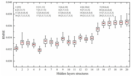
Figure 5.
Prediction RMSEs for different hidden layer structures (neural network model for May).
Moreover, a genetic algorithm [66] was also used to optimize the values of the weights and biases in the BP neural network model and to minimize the prediction errors due to the random assignment of weights and biases. The results show that the performances of the BPNN models were significantly improved by the genetic algorithm, and the determination coefficients (R2) of the GA-BPNN models (0.46, 0.73, 0.68, 0.62, and 0.47 for May to September, respectively) were higher than those of the BPNN models (0.42, 0.72, 0.64, 0.6, and 0.44 for May to September, respectively) (Figure 6).
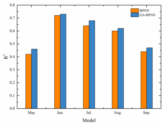
Figure 6.
Comparison of the performances of the BPNN and GA-BPNN models for each month.
2.2.2. Statistical-Based Temporal Filter
To generate a spatiotemporally continuous MPF dataset for Arctic sea ice, a statistical-based temporal filter was utilized to fill in the data gaps in the GA-BPNN predictions. In our previous study, a statistical-based temporal filter was used to generate spatiotemporally continuous datasets of the land surface albedo [67,68]. The daily land surface albedo can be reconstructed based on a weighted combination of the albedo estimated from remote sensing data, the albedo estimated based on the relationships between neighboring days, and the albedo climatology (multi-year mean albedo).
However, because the MPF of Arctic is highly spatiotemporally dynamic and has large inter-annual variability, the MPF climatology was not used in this study, and the missing data were mainly filled based on the relationships between neighboring days. It is clear that the MPFs of neighboring days are closely correlated, and this can be explicitly expressed as a linear relationship [67]:
where is the MPF on kth day, is the MPF at (k + ∆k)th day, ∆k is the temporal interval between the neighboring days (−4 ≤ ∆k ≤ 4 for this study), and are the regression coefficients of the linear regression, and is the regression residuals. These parameters can be derived based on the priori statistics of the MPF climatology [67]:
where (k = 1, 2, …, 140, k denotes the sequential days from 8 May to 24 September) and are the mean MPFs of the multi-year data on kth and (k + ∆k)th days, and are the standard deviations of the MPF on kth and (k + ∆k)th days, (= −4, −3, …, 3, 4) is correlation coefficient for the MPFs of the neighboring days with an interval of ∆k, and is the RMSE between the MPFs of kth and (k + ∆k)th days. The above-mentioned priori statistics of the MPF climatology can be derived from statistical analysis of the UB-MPF dataset.
Finally, the MPF of kth day can be reconstructed through the weighted combination of MPFs estimated using the GA-BPNN model and the MPFs predicted by the statistical relationships between the neighboring days:
where is the reconstructed MPF on kth day, is the RMSE between the MPFs on kth and (k + ∆k)th days, and and are the standard derivations of the MPFs estimated using the GA-BPNN model for kth and (k + ∆k)th days.
3. Results and Discussion
3.1. Accuracy of the GA-BPNN Model
The sophisticated non-linear relationship between the directional surface reflectance (seven bands of MODIS data), incident/viewing geometries (SZA, VZA, SAA, and VAA), and MPF can be efficiently constructed using the GA-BPNN model. The validation results show that the GA-BPNN models have good performance in terms of predicting the MPF of Arctic sea ice, with an R2 of 0.76 and an RMSE of 0.05 (Figure 7). The predicted RMSEs of the GA-BPNN models for May to September are 0.032, 0.054, 0.059, 0.048, and 0.049, respectively (Figure 8). The GA-BPNN predictions are in good agreement with the validation dataset (i.e., the true MPF) in June, July, and August, and most of the estimates plot close to the 1-to-1 line.
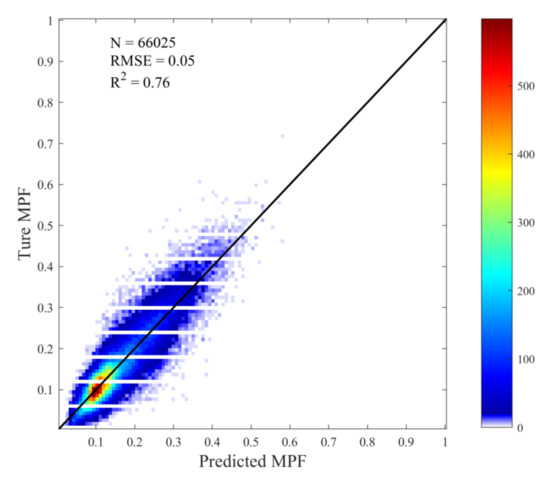
Figure 7.
Performance of the GA-BPNN models for all the data (from May to September). The color gradient represents the density of the scatter in each grid.
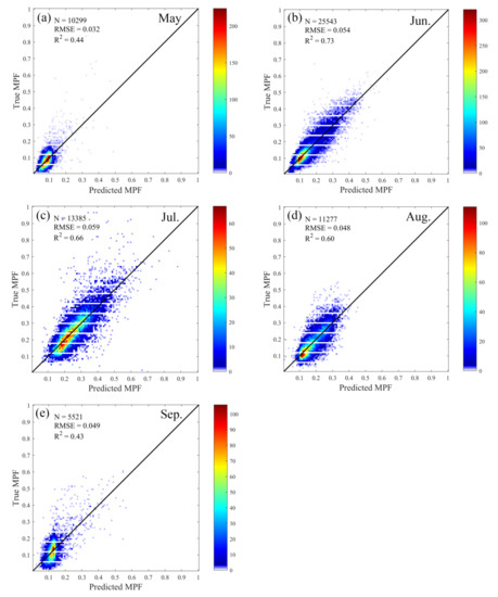
Figure 8.
Performances of the GA-BPNN models for each month (from May to September):(a) May, (b) June, (c) July, (d) August, and (e) September. The color gradient represents the density of the scatter in each grid.
The validation results exhibit relatively lower R2 values for May and September, which is mainly because the MPFs in May and September are much lower than those in June, July, and August, and larger uncertainties in the MPF can be obtained when the MPF is lower.
3.2. Accuracy of Statistical-Based Temporal Filter
The MPF datasets for Arctic sea ice before and after gap filling are shown in Figure 9 and Figure 10, respectively. The original dataset generated using the GA-BPNN model is not spatiotemporally continuous owing to cloud obscuration. However, the data gaps can be efficiently filled by the statistical-based temporal filter, and the generated NENU-MPF dataset represents the spatiotemporal dynamics of MPF of the Arctic sea ice well.
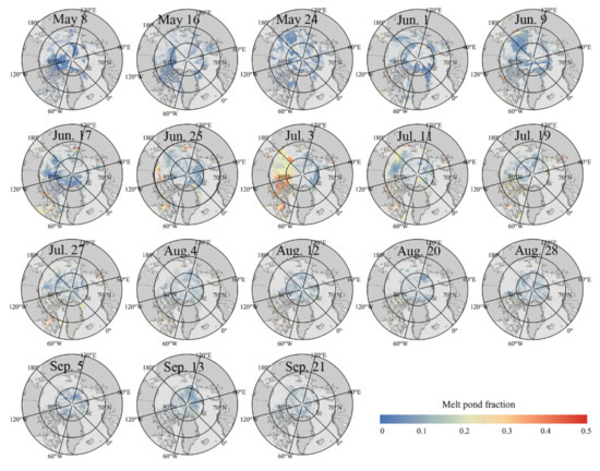
Figure 9.
MPF dataset for Arctic sea ice without gap-filling (raw data derived using the GA-BPNN model) in 2017. For brevity, only the MPFs every eight days from 8 May to 24 September 2017, are shown, and the light grey color indicates the missing data due to cloud obscuration.
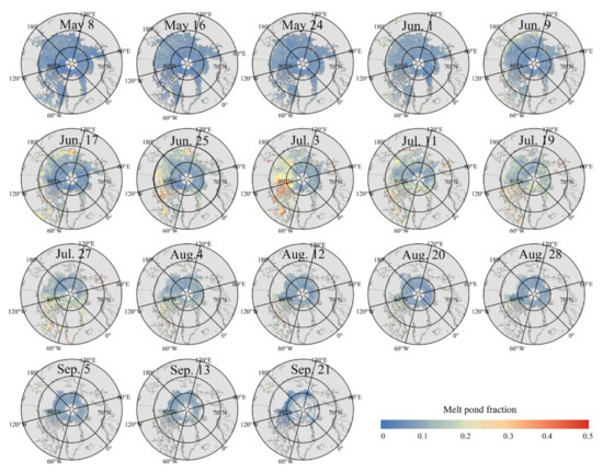
Figure 10.
Gap-filled MPF dataset for Arctic sea ice (NENU-MPF dataset) in 2017. For brevity, only the MPFs every eight days from 8 May to 24 September 2017 are shown.
From May to early June, the MPFs were relatively low, and the melt ponds mainly appeared in the northern coastal areas of Asia and North America. Then, from mid-June to mid-July, the MPFs increased significantly in the first-year ice zone (Beaufort Sea, East Siberian Sea, and Laptev Sea) as the air temperature increased. Finally, from late July to September, the MPFs decreased significantly and reverted to the level during the pre-melting season.
An example of MPF data processed using the statistical-based temporal filter is shown in Figure 11. As can be seen from Figure 11, numerous data gaps existed in the original MPF dataset derived using the GA-BPNN model; however, a spatiotemporally continuous dataset without missing data was obtained by applying the statistical-based temporal filter.
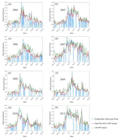
Figure 11.
Example of MPF data processed using the statistical-based temporal filter (137°46′0.41″W, 74°33′9.33″N) in (a) 2004, (b) 2005, (c) 2006, (d) 2007, (e) 2008, (f) 2009, (g) 2010, and (h) 2011, respectively.
Moreover, the temporal variations in the NENU-MPF dataset are similar to the reference UB-MPF dataset, which indicates that the MPF data missing due to cloud obscuration can be well reconstructed using the statistical-based temporal filter. Figure 12 presents a comparison of the gap-filled MPF with the reference UB-MPF dataset. The comparison results show that the gap-filled MPF derived using the statistical-based temporal filter is consistent with the UB-MPF dataset, with an R2 of 0.43, an RMSE of 0.047, and a bias of −0.022. Its accuracy is lower than that of the GA-BPNN model. However, with the advantage of generating spatiotemporally continuous dataset, the reconstruction accuracy of the statistical-based temporal filter is acceptable at most times.
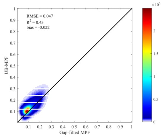
Figure 12.
Comparison of gap-filled MPF with the UB-MPF dataset. The color gradient represents the density of the scatter in each grid.
3.3. Validation Results
The validation results of the NENU-MPF dataset with the ASIMPSM dataset are shown in Figure 13. The NENU-MPF dataset is roughly consistent with the MPF derived from the images collected in the Beaufort Sea, East Siberian Sea, Canadian Arctic, and Fram Strait during 2000–2001, with an RMSE of 0.08 and an R2 of 0.58. The MEDEA, IceWatch, TransArc, and HOTRAX datasets were used to validate the NENU-MPF dataset, and the UB-MPF dataset was also used as a reference for comparison. The validation results show that the NENU-MPF dataset is roughly consistent with the MEDEA (R2 = 0.41, RMSE = 0.102, and bias = −0.04), IceWatch (R2 = 0.60, RMSE = 0.105, and bias = 0.05), TransArc (R2 = 0.027, RMSE = 0.21, and bias = 0.174), and HOTRAX (R2 = 0.20, RMSE = 0.098, and bias = 0.007) datasets (Figure 14).
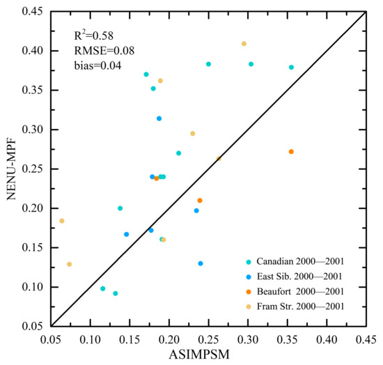
Figure 13.
Validation of the NENU-MPF dataset against the ASIMPSM dataset.
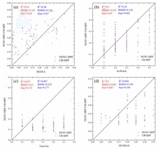
Figure 14.
Validation of the NENU-MPF dataset against the (a) MEDEA, (b) IceWatch, (c) TransArc, and (d) HOTRAX datasets.
The results of the validation against the UB-MPF dataset indicate that it has an accuracy comparable with that of the NENU-MPF dataset and is roughly consistent with the MEDEA (R2 = 0.39, RMSE = 0.119, and bias = −0.07), IceWatch (R2 = 0.26, RMSE = 0.126, and bias = 0.002), TransArc (R2 = 0.007, RMSE = 0.219, and bias = 0.177), and HOTRAX (R2 = 0.004, RMSE = 0.149, and bias = 0.106) datasets. The satellite-based measurements (ASIMPSM and MEDEA datasets) are more consistent with our results than with the ship-based measurements (IceWatch, TransArc, and HOTRAX datasets). We also found that the TransArc dataset is not consistent with the NENU-MPF and UB-MPF datasets, which is mainly due to the discrepancy between the spatial resolutions of the remote sensing datasets (12.5 km) and the footprints of the ship-based measurements (50 m to 10 km, which mainly depends on the horizontal visibility and height of the observation position).
3.4. Comparison Results
The results of the comparisons of the NENU-MPF dataset with the UB-MPF, BNU-MPF, UB-OLCI, and UH-MPF datasets are shown in Figure 15. The results show that the NENU-MPF dataset is consistent with the UB-MPF dataset, with an R2 of 0.70, an RMSE of 0.052, and a bias of −0.02, which is reasonable because the UB-MPF dataset was used as the training dataset for the GA-BPNN model. The NENU-MPF dataset is also consistent with the BNU-MPF dataset, with an R2 of 0.40, an RMSE of 0.06, and a bias of −0.011.
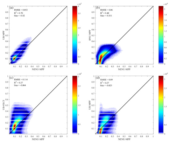
Figure 15.
Comparison of NENU-MPF dataset with the (a) UB-MPF, (b) BNU-MPF, (c) UB-OLCI, and (d) UH-MPF datasets. The color gradient represents the density of the scatter in each grid.
While the consistencies between the NENU-MPF and UB-OLCI datasets (R2 = 0.27, RMSE = 0.114, and bias = −0.064) and the NENU-MPF and UH-MPF datasets (R2 = 0.27, RMSE = 0.09, and bias = −0.025) are relatively poor. The discrepancies between the NENU-MPF and UH-MPF datasets are mainly due to the different algorithms used to estimate the MPF. Moreover, the spectral unmixing method used in the UH-MPF dataset assumes that the spectral reflectance of the sea ice components is invariant [54], which may result in a large error when the depth and area of the melt ponds increase.
The annual mean MPF values derived using the UB-MPF, UH-MPF, NENU-MPF, and BNU-MPF datasets from 2002 to 2020 are shown in Figure 16. As there are large data gaps in the UH-MPF, BNU-MPF, and UB-MPF during 2000–2001, the annual mean MPF values of the Arctic sea ice during 2000–2001 are not shown in Figure 16.
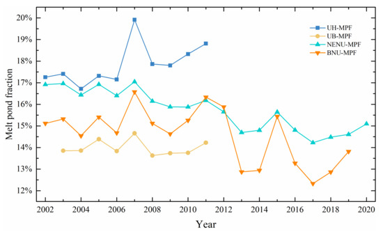
Figure 16.
The annual-mean MPF derived from the different datasets (UH-MPF, UB-MPF, NENU-MPF, and BNU-MPF datasets from May to September). Only the pixels with valid MPF values were used.
To eliminate the missing data, the original UB-MPF dataset was filtered using a running mean of 8 days before the annual mean MPF was calculated. To minimize the influence of the missing data, only the pixels with valid MPF values were used. In addition, the UB-OLCI dataset was not compared with the other datasets due to the limited spatial coverage of this dataset. The results show that the NENU-MPF, UB-MPF, BNU-MPF, and UH-MPF exhibit MPF trends of −0.0015/yr, −0.00005/yr, –0.0014/yr, and 0.0018/yr, respectively.
The NENU-MPF dataset has a much longer temporal span than the UB-MPF and UH-MPF datasets, and its decreasing trend is consistent with that of the BNU-MPF dataset from 2002 to 2020. It is noticeable that the values of the UH-MPF dataset are much higher than those of the other datasets, and it exhibits a contrast increasing MPF trend, which is not consistent with the MPF trends derived from the UB-MPF, NENU-MPF, and BNU-MPF datasets. The discrepancies between these datasets can be explained by the differences in the estimation methods used, as well as the degree of spatiotemporal continuity (or data gaps) of these datasets.
The multi-year mean temporal evolutions of the MPF derived from the UH-MPF, UB-MPF, NENU-MPF, and BNU-MPF datasets from May to September during 2003–2011 are shown in Figure 17. For all of the MPF datasets, the MPF initially increases and then decreases with time. The MPF of the Arctic sea ice is lowest in early May, rapidly increases in June, and reaches the maximum MPF value in late June to mid-July. Then, the MPF decreases in August and September, and it falls to the lowest value in September. These datasets exhibit similar temporal trends in the MPF, and the UH-MPF and NENU-MPF datasets present the highest values in the peak season, followed by the BNU-MPF and UB-MPF.
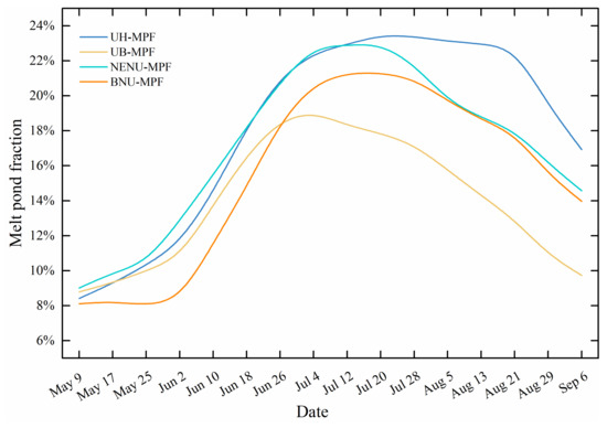
Figure 17.
Multi-year mean temporal evolution of the MPF derived from the UH-MPF, UB-MPF, NENU-MPF, and BNU-MPF datasets from May to September during 2003–2011. Only the pixels with valid MPF values were used.
In addition, the UH-MPF dataset exhibits an approximate one-month lag in the decline of the MPF, which is not consistent with the other three datasets. The temporal variations in the MPF of the Arctic sea ice derived from the NENU-MPF datasets from 2000 to 2020 are shown in Figure 18. The regional mean MPF varies from approximate 6% to 20% exhibits a large standard derivation from late June to early August. The newly generated NENU-MPF dataset accurately characterizes the temporal evolution of the MPF and captures the phenomena of abnormal high MPF values in 2007.
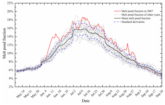
Figure 18.
Temporal variations in the MPF of the Arctic sea ice derived from the NENU-MPF datasets from 2000 to 2020. The pixels over the entire Arctic sea ice region were used.
3.5. Discussion
The temporal span and spatiotemporal continuity are crucial characteristics of MPF datasets for Arctic sea ice, which influence the reliability of the long-term trends derived from satellite observations. As most of the geophysical parameters of the Earth vary with climatic and environmental factors, the trends of the geophysical parameters can be significantly influenced by the general circulation and atmospheric oscillations [69], as well as the data gaps caused by cloud obscuration [67], and thus datasets with longer temporal span and more spatiotemporal continuity are required to more accurately determine the MPF trend.
The comparison results indicate that the newly generated NENU-MPF dataset has a much longer temporal span (from 2000 to 2020) than that of UB-MPF (from 2002 to 2011) and UH-MPF (from 2000 to 2011) datasets and is more spatiotemporally continuous compared to the other datasets. Thus, it has potential advantages in term of representing the dynamics and evolution of the MPF of Arctic sea ice more realistically.
For example, the long-term trend in MPF of the Arctic sea ice derived from the NENU-MPF dataset can be considered more accurate and reliable, and the NENU-MPF dataset can be used as a reference for calibrating and developing the melt ponds evolution models [70]. In addition, there are also many potential applications for the newly generated MPF dataset of Arctic sea ice [50], such as improving the treatment of sea ice albedo in the global climate models, qualifying the uncertainty of sea ice concentration dataset, analyzing the interannual variability in melt processes of Arctic sea ice, and estimating the contribution of melt ponds to the sea ice albedo feedback mechanism.
Although differences in the MPF values of the different datasets were identified, a significant decreasing MPF trend can be found in most of these datasets (Figure 15). The large bias and opposite trend of the UH-MPF dataset are mainly due to the assumption in the spectral unmixing method that the spectral reflectance of the sea ice components is invariant [54], which resulted in large uncertainties in estimating the MPF when the sea ice surface changed significantly during the melting season.
In addition, the data gaps due to cloud obscuration also increased the uncertainty of the MPF trends derived from these datasets. The significant decreasing trend of the MPF in the Arctic can be explained by the decline in the sea ice extent, and the fact that the melted area of first-year ice (where the melt ponds mainly appear) has increased dramatically due to global warming, leading to a decrease in the MPF of the Arctic sea ice in recent decades [70].
In this study, a GA-BPNN model and statistical temporal filter were applied to improve the temporal span and spatiotemporal continuity of the MPF dataset. Compared to previous studies that did not consider the effect of the reflectance anisotropic of the melt ponds, in this study, the bidirectional reflectance distribution (BRDF) characteristics of the melt ponds were fully considered using the directional reflectance/geometries and GA-BPNN model. Our knowledge of the reflectance anisotropic properties of the melt ponds was derived from the physical-based UB-MPF dataset. In addition, the missing data due to cloud obscuration were efficiently filled using a statistical-based temporal filter, and the spatiotemporal continuity of the MPF dataset was significantly improved.
The shortcomings of this study and the issues that need to be addressed in the future are listed as follows:
(1) The spatial resolution and validation accuracy of the proposed NENU-MPF dataset need to be improved in the future. Owing to the inconsistency of the footprints of the MPF dataset and the validation data, our results are only roughly consistent with the validation dataset. To address this issue, a labeled dataset for melt ponds in the Arctic derived from high-spatial-resolution satellite imageries is needed [71]. There is a potential to generate a more accurate MPF dataset using deep learning and a training dataset, and the validation of the MPF datasets would also benefit from a labeled dataset of melt ponds. In addition, developing new validation and uncertainty qualification methods [72,73] over Arctic sea ice region are also required in future studies.
(2) Although data gaps can be efficiently filled using the statistical-based temporal filter, the gap filling methods with higher accuracy are still required for generating spatiotemporally continuous MPF datasets. In this study, only the relationship between the neighboring days was used in the gap filling of the MPF dataset, and this assumption may be invalid due to snow fall/melt, and sea ice drifts, which would result in a relatively poor gap filling accuracy under certain circumstances. In the future, the temporal correlation, spatial autocorrelation, and the relationship with the passive remote-sensing data can be incorporate to generate a seamless MPF dataset [74]. In addition, the deep-learning and inpainting methods can also be used for developing new gap filling methods, which have shown promising results in recent studies [75,76].
(3) Satellite observations acquired by multiple platforms and sensors can be jointly used to extend the temporal span of the MPF dataset. The method proposed in this study can be adapted to other remote sensing data, e.g., Advanced Very High Resolution Radiometer (AVHRR) and Visible Infrared Imaging Radiometer Suite (VIIRS) data. The combined use of AVHRR, MODIS, and VIIRS data has the potential to extend the temporal span to more than 40 years (from 1981 to the present).
4. Conclusions
In this study, we generated a long-term spatiotemporally continuous MPF dataset for Arctic sea ice from MODIS data from 2000 to 2020. First, a non-linear relationship between the MODIS directional reflectance/geometries and the UB-MPF dataset was successfully constructed using a GA-BPNN model. Then, the missing data due to cloud obscuration were efficiently filled using a statistical-based temporal filter. Finally, the generated NENU-MPF dataset was validated using satellite-based and ship-based measurements and was compared with other published datasets, such as the UB-MPF, UB-OLCI, UH-MPF, and BNU-MPF datasets.
The MPF values of Arctic sea ice were accurately predicted using the GA-BPNN model (R2 = 0.76, RMSE = 0.05), and the missing data were filled in using the statistical-based temporal filter. The validation and comparison results showed that the NENU-MPF dataset was consistent with the validation measurements as well as the UB-MPF (R2 = 0.70, RMSE = 0.052) and BNU-MPF (R2 = 0.40, RMSE = 0.06) datasets. The newly generated NENU-MPF dataset was demonstrated to be more spatiotemporally continuous with a longer temporal span (21 years).
The results of this study improve our knowledge of the long-term variations in Arctic sea ice over recent decades. The newly generated NENU-MPF dataset demonstrated great advantages in providing accurate and reliable trends and interannual variability in the MPF of Arctic sea ice during the recent two decades and can also be used as a fundamental dataset in studies of global climate change and the surface energy budget.
Author Contributions
Conceptualization, Y.Q.; methodology, Z.P., Y.D., Y.Q., M.W. and X.L.; results validation, Z.P., Y.D. and M.W.; investigation, Z.P., Y.D. and M.W.; data curation, Z.P. and Y.D.; writing—original draft, Z.P.; writing—review editing, Y.Q. and X.L.; visualization, Z.P., M.W. and Y.Q.; funding acquisition, Y.Q. All authors have read and agreed to the published version of the manuscript.
Funding
This work was financially supported by the National Key Research and Development Program of China (2020YFA0714102) and the National Natural Science Foundation of China (41971287 and 41601349).
Institutional Review Board Statement
Not applicable.
Informed Consent Statement
Not applicable.
Data Availability Statement
The MODIS daily surface reflectance data can be downloaded from https://www.earthdata.nasa.gov, accessed on 1 October 2021, the UB-MPF dataset can be downloaded from https://seaice.uni-bremen.de/data/meris/gridded/, accessed on 1 October 2021, the UB-OLCI dataset can be downloaded from https://seaice.uni-bremen.de/data/olci/, accessed on 1 October 2021, the UH-MPF dataset can be downloaded from https://www.cen.uni-hamburg.de/icdc/data/cryosphere/arctic-meltponds.html, accessed on 1 October 2021, the BNU-MPF dataset can be downloaded from https://doi.pangaea.de/10.1594/PANGAEA.933280, accessed on 1 October 2021, the ASIMPSM dataset can be downloaded from https://nsidc.org/data/G02159/versions/1, accessed on 1 October 2021, the MEDEA dataset can be downloaded from http://psc.apl.uw.edu/melt-pond-data/, accessed on 1 October 2021, the IceWatch dataset can be downloaded from https://icewatch.met.no/, accessed on 1 October 2021, the TransArc dataset can be downloaded from https://doi.pangaea.de/10.1594/PANGAEA.803312, accessed on 1 October 2021, and the NENU-MPF dataset can be downloaded from https://doi.org/10.5281/zenodo.6888170, accessed on 23 July 2022.
Acknowledgments
The authors would like to thank the University of Bremen, University of Hamburg, and Beijing Normal University for providing the MPF datasets, as well as Perovich for providing the measured data.
Conflicts of Interest
The authors declare no conflict of interest.
References
- Eicken, H.; Grenfell, T.C.; Perovich, J.A.; Richter-Menge, J.A.; Frey, K. Hydraulic controls of summer Arctic pack ice albedo. J. Geophys. Res. Ocean. 2004, 109, C08007. [Google Scholar] [CrossRef]
- Li, P. The Arctic sea ice and climate change. J. Glaciol. Geocryol. 1996, 18, 74–82. [Google Scholar]
- Taskjelle, T.R.; Hudson, S.R.; Granskog, M.A.; Nicolaus, M.; Lei, R.; Gerland, S.; Stamnes, J.J.; Hamre, B.R. Spectral albedo and transmittance of thin young Arctic sea ice. J. Geophys. Res. Ocean. 2016, 121, 540–553. [Google Scholar] [CrossRef]
- Malinka, A.; Zege, E.; Istomina, L.; Heygster, G.; Spreen, G.; Perovich, D.; Polashenski, C. Reflective properties of melt ponds on sea ice. Cryosphere 2018, 12, 1921–1937. [Google Scholar] [CrossRef]
- Flocco, D.; Feltham, D.L. A continuum model of melt pond evolution on Arctic sea ice. J. Geophys. Res. Ocean. 2007, 112, C08016. [Google Scholar] [CrossRef]
- Polashenski, C.; Perovich, D.; Courville, Z. The mechanisms of sea ice melt pond formation and evolution. J. Geophys. Res. Ocean. 2012, 117, C01001. [Google Scholar] [CrossRef]
- Fetterer, F.; Untersteiner, N. Observations of melt ponds on Arctic sea ice. J. Geophys. Res. Ocean. 1998, 103, 24821–24835. [Google Scholar] [CrossRef]
- Peng, Z.; Ding, Y.; Qu, Y.; Wang, M.; Li, X. An artificial neural network framework for estimating melt pond fraction of Arctic sea ice from MODIS data. In Proceedings of the IEEE 2022 International Geoscience and Remote Sensing Symposium (IGARSS 2022), Kuala Lumpur, Malaysia, 18 July 2022. [Google Scholar]
- Perovich, D.; Grenfell, T.; Light, B.; Elder, B.; Harbeck, J.; Polashenski, C.; Tucker, W.; Stelmach, C. Transpolar observations of the morphological properties of Arctic sea ice. J. Geophys. Res. Ocean. 2009, 114, C00A04. [Google Scholar] [CrossRef]
- Perovich, D.K.; Grenfell, T.C.; Light, B.; Hobbs, P.V. Seasonal evolution of the albedo of multiyear Arctic sea ice. J. Geophys. Res. Ocean. 2002, 107, 8044. [Google Scholar] [CrossRef]
- Grenfell, T.C.; Perovich, D.K. Seasonal and spatial evolution of albedo in a snow-ice-land-ocean environment. J. Geo Phys. Res. Ocean. 2004, 109, C01001. [Google Scholar] [CrossRef]
- Inoue, J.; Curry, J. Application of aerosondes to melt-pond observations over Arctic sea ice. J. Atmos. Ocean. Technol. 2008, 25, 327–334. [Google Scholar] [CrossRef]
- Perovich, D.K.; Polashenski, C. Albedo evolution of seasonal Arctic sea ice. Geophys. Res. Lett. 2012, 39, L08501. [Google Scholar] [CrossRef]
- Hanesiak, J.M.; Barber, D.G.; De Abreu, R.A.; Yackel, J.J. Local and regional albedo observations of arctic first-year sea ice during melt ponding. J. Geophys. Res. Ocean. 2001, 106, 1005–1016. [Google Scholar] [CrossRef]
- Grenfell, T.C.; Maykut, G.A. The optical properties of ice and snow in the Arctic Basin. J. Glaciol. 1977, 18, 445–463. [Google Scholar] [CrossRef]
- Eicken, H.; Krouse, H.R.; Kadko, D.; Perovich, D.K. Tracer studies of pathways and rates of meltwater transport through Arctic summer sea ice. J. Geophys. Res. Ocean. 2002, 107, 21–22. [Google Scholar] [CrossRef]
- Thackeray, C.W.; Hall, A. An emergent constraint on future Arctic sea-ice albedo feedback. Nat. Clim. Chang. 2019, 9, 972–978. [Google Scholar] [CrossRef]
- Wendisch, M.; Brückner, M.; Burrows, J.; Crewell, S.; Dethloff, K.; Ebell, K.; Lüpkes, C.; Macke, A.; Notholt, J.; Quaas, J.; et al. Understanding Causes and Effects of Rapid Warming in the Arctic. Eos 2017, 98. [Google Scholar] [CrossRef]
- Flocco, D.; Schroeder, D.; Feltham, D.L.; Hunke, E.C. Impact of melt ponds on Arctic sea ice simulations from 1990 to 2007. J. Geophys. Res. Ocean. 2012, 117, C09032. [Google Scholar] [CrossRef]
- Schroeder, D.; Feltham, D.L.; Flocco, D.; Tsamados, M. September Arctic sea-ice minimum predicted by spring melt-pond fraction. Nat. Clim. Chang. 2014, 4, 353–357. [Google Scholar] [CrossRef]
- Howell, S.; Scharien, R.; Landy, J.; Brady, M. Spring melt pond fraction in the Canadian Arctic Archipelago predicted from RADARSAT-2. Cryosphere 2020, 14, 4675–4686. [Google Scholar] [CrossRef]
- Ding, Y.; Cheng, X.; Liu, J.; Hui, F.; Wang, Z.; Chen, S. Retrieval of melt pond fraction over Arctic sea ice during 2000—2019 Using an Ensemble-Based Deep Neural Network. Remote Sens. 2020, 12, 2746. [Google Scholar] [CrossRef]
- Feng, J.; Zhang, Y.; Cheng, Q.; Wong, K.; Li, Y.; Yeu Tsou, J. Effect of melt ponds fraction on sea ice anomalies in the Arctic Ocean. Int. J. Appl. Earth Obs. Geoinf. 2021, 98, 102297. [Google Scholar] [CrossRef]
- Birnbaum, G.; Dierking, W.; Hartmann, J.; Lüpkes, C.; Ehrlich, A.; Garbrecht, T.; Sellmann, L. The campaign MELTEX with research aircraft “POLAR 5” in the Arctic in 2008. Rep. Polar Mar. Res. 2009, 593, 3–85. [Google Scholar]
- Derksen, C.; Piwowar, J.; LeDrew, E. Sea-ice melt-pond fraction as determined from low level aerial photographs. Arct. Alp. Res. 1997, 29, 345–351. [Google Scholar] [CrossRef]
- Rösel, A.; Kaleschke, L. Comparison of different retrieval techniques for melt ponds on Arctic sea ice from Landsat and MODIS satellite data. Ann. Glaciol. 2011, 52, 185–191. [Google Scholar] [CrossRef]
- El Naggar, S.; Garrity, C.; Ramseier, R.O. The modelling of sea ice melt-water ponds for the high Arctic using an airborne line scan camera, and applied to the satellite special sensor microwave/imager (SSM/I). Int. J. Remote Sens. 1998, 19, 2373–2394. [Google Scholar] [CrossRef]
- Tschudi, M.; Curry, J.; Maslanik, J. Determination of areal surface-feature coverage in the Beaufort Sea using aircraft video data. Ann. Glaciol. 1997, 25, 434–438. [Google Scholar] [CrossRef]
- Makynen, M.; Kern, S.; Roesel, A.; Pedersen, L.T. On the Estimation of melt pond fraction on the Arctic sea ice with ENVISAT WSM Images. IEEE Trans. Geosci. Remote Sens. 2014, 52, 7366–7379. [Google Scholar] [CrossRef]
- Fors, A.S.; Divine, D.V.; Doulgeris, A.P.; Renner, A.H.H.; Gerland, S. Signature of Arctic first-year ice melt pond fraction in X-band SAR imagery. Cryosphere 2017, 11, 755–771. [Google Scholar] [CrossRef]
- Guo, J.; Sun, B.; Li, Q.; Lei, R.; Li, B.; Li, N. Application and development of the buoys based on polar sea ice. Chin. J. Polar Res. 2011, 23, 149–157. [Google Scholar] [CrossRef]
- Zhang, R.; Ke, C.; Xie, H.; Sun, B. Surface Albedo Measurements over Sea Ice in the Arctic Ocean during Summer 2010. Chin. J. Polar Res. 2012, 24, 299–306. [Google Scholar] [CrossRef]
- Sankelo, P.; Haapala, J.; Heiler, I.; Rinne, E. Melt pond formation and temporal evolution at the drifting station Tara during summer 2007. Polar Res. 2010, 29, 311–321. [Google Scholar] [CrossRef]
- Nicolaus, M.; Katlein, C.; Maslanik, J.A.; Hendricks, S. Sea ice conditions during the POLARSTERN cruise ARK-XXVI/3 (TransArc) in 2011. Geophys. Res. Lett. 2012, 39, L24501. [Google Scholar] [CrossRef]
- Xie, H.; Lei, R.; Ke, C.; Wang, H.; Li, Z.; Zhao, J.; Ackley, S.F. Summer sea ice characteristics and morphology in the Pacific Arctic sector as observed during the CHINARE 2010 cruise. Cryosphere 2013, 7, 1057–1072. [Google Scholar] [CrossRef]
- Wang, M.; Su, J.; Li, T.; Wang, X.; Ji, Q.; Cao, Y.; Lin, L.; Liu, Y. Study on the method of extracting Arctic melt pond and roughness information on sea ice surface based on UAV observation. Chin. J. Polar Res. 2017, 29, 436–445. [Google Scholar]
- Miao, X.; Xie, H.; Ackley, S.; Perovich, D.; Ke, C. Object-based detection of Arctic sea ice and melt ponds using high spatial resolution aerial photographs. Cold Reg. Sci. Technol. 2015, 119, 787–791. [Google Scholar] [CrossRef]
- Tschudi, M.A.; Curry, J.A.; Maslanik, J.A. Airborne observations of summertime surface features and their effect on surface albedo during FIRE/SHEBA. J. Geophys. Res. Atmos. 2001, 106, 15335–15344. [Google Scholar] [CrossRef]
- Markus, T.; Cavalieri, D.J.; Ivanoff, A. The potential of using Landsat 7 ETM+ for the classification of sea-ice surface conditions during summer. Ann. Glaciol. 2002, 34, 415–419. [Google Scholar] [CrossRef][Green Version]
- Markus, T.; Cavalieri, D.J.; Tschudi, M.A.; Ivanoff, A. Comparison of aerial video and Landsat 7 data over ponded sea ice. Remote Sens. Environ. 2003, 86, 458–469. [Google Scholar] [CrossRef]
- Wright, N.C.; Polashenski, C.M. Open-source algorithm for detecting sea ice surface features in high-resolution optical imagery. Cryosphere 2018, 12, 1307–1329. [Google Scholar] [CrossRef]
- Yackel, J.J.; Nandan, V.; Mahmud, M.; Scharien, R.; Kang, J.W.; Geldsetzer, T. A spectral mixture analysis approach to quantify Arctic first-year sea ice melt pond fraction using QuickBird and MODIS reflectance data. Remote Sens. Environ. 2018, 204, 704–716. [Google Scholar] [CrossRef]
- Wang, M.; Su, J.; Landy, J.; Leppäranta, M.; Guan, L. A new algorithm for sea ice melt pond fraction estimation from high-resolution optical satellite imagery. J. Geophys. Res. Ocean. 2020, 125, e2019JC015716. [Google Scholar] [CrossRef]
- Huang, W.; Lu, P.; Lei, R.; Xie, H.; Li, Z. Melt pond distribution and geometry in high Arctic sea ice derived from aerial investigations. Ann. Glaciol. 2016, 57, 105–118. [Google Scholar] [CrossRef]
- Perovich, D.K. Aerial observations of the evolution of ice surface conditions during summer. J. Geophys. Res. 2002, 107, 21–24. [Google Scholar] [CrossRef]
- Qin, Y.; Su, J.; Wang, M. Melt pond retrieval based on the LinearPolar algorithm using Landsat data. Remote Sens. 2021, 13, 4674. [Google Scholar] [CrossRef]
- Lu, P.; Li, Z.; Cheng, B.; Lei, R.; Zhang, R. Sea ice surface features in Arctic summer 2008: Aerial observations. Remote Sens. Environ. 2010, 114, 693–699. [Google Scholar] [CrossRef]
- Renner, A.H.H.; Gerland, S.; Haas, C.; Spreen, G.; Beckers, J.F.; Hansen, E.; Nicolaus, M.; Goodwin, H. Evidence of Arctic sea ice thinning from direct observations. Geophys. Res. Lett. 2014, 41, 5029–5036. [Google Scholar] [CrossRef]
- Arntsen, A.E.; Song, A.J.; Perovich, D.K.; Richter-Menge, J.A. Observations of the summer breakup of an Arctic sea ice cover. Geophys. Res. Lett. 2015, 42, 8057–8063. [Google Scholar] [CrossRef]
- Tschudi, M.A.; Maslanik, J.A.; Perovich, D.K. Derivation of melt pond coverage on Arctic sea ice using MODIS observations. Remote Sens. Environ. 2008, 112, 2605–2614. [Google Scholar] [CrossRef]
- Istomina, L.; Heygster, G.; Huntemann, M.; Marks, H.; Melsheimer, C.; Zege, E.; Malinka, A.; Prikhach, A.; Katsev, I. Melt pond fraction and spectral sea ice albedo retrieval from MERIS data—Part 2: Case studies and trends of sea ice albedo and melt ponds in the Arctic for years 2002-2011. Cryosphere 2015, 9, 1567–1578. [Google Scholar] [CrossRef]
- Istomina, L.; Marks, H.; Huntemann, M.; Heygster, G.; Spreen, G. Improved cloud detection over sea ice and snow during Arctic summer using MERIS data. Atmos. Meas. Technol. 2020, 13, 6459–6472. [Google Scholar] [CrossRef]
- Lee, S.; Stroeve, J.; Tsamados, M.; Khan, A.L. Machine learning approaches to retrieve pan-Arctic melt ponds from visible satellite imagery. Remote Sens. Environ. 2020, 247, 111919. [Google Scholar] [CrossRef]
- Rösel, A.; Kaleschke, L.; Birnbaum, G. Melt ponds on Arctic sea ice determined from MODIS satellite data using an artificial neural network. Cryosphere 2012, 6, 431–446. [Google Scholar] [CrossRef]
- Rösel, A.; Kaleschke, L.; Kern, S.E. Gridded Melt Pond Cover Fraction on Arctic Sea Ice derived from TERRA-MODIS 8-Day Composite Reflectance Data Bias Corrected Version 02. World Data Center for Climate (WDCC) at DKRZ. Available online: https://www.wdc-climate.de/ui/entry?acronym=MODIS__Arctic__MPF_V02 (accessed on 1 October 2021).
- Zege, E.; Malinka, A.; Katsev, I.; Prikhach, A.; Heygster, G.; Istomina, L.; Birnbaum, G.; Schwarz, P. Algorithm to retrieve the melt pond fraction and the spectral albedo of Arctic summer ice from satellite optical data. Remote Sens. Environ. 2015, 163, 153–164. [Google Scholar] [CrossRef]
- Kokhanovsky, A.; Zege, E. Scattering Optics of Snow. Appl. Opt. 2004, 43, 1589–1602. [Google Scholar] [CrossRef]
- Malinka, A.; Zege, E.; Heygster, G.; Istomina, L. Reflective properties of white sea ice and snow. Cryosphere 2016, 10, 2541–2557. [Google Scholar] [CrossRef]
- Istomina, L.; Heygster, G.; Huntemann, M.; Schwarz, P.; Birnbaum, G.; Scharien, R.; Polashenski, C.; Perovich, D.; Zege, E.; Malinka, A.; et al. Melt pond fraction and spectral sea ice albedo retrieval from MERIS data-Part 1: Validation against in situ, aerial, and ship cruise data. Cryosphere 2015, 9, 1551–1566. [Google Scholar] [CrossRef]
- Istomina, L. Retrieval of sea ice surface melt using OLCI data onboard Sentinel-3. In AGU Fall Meeting 2020; American Geophysical Union: Washington, DC, USA, 2020. [Google Scholar]
- Ding, Y.; Liu, J.; Cheng, X.; Chen, S. Melt pond fraction over Arctic sea ice during 2000–2019. PANGAEA 2021. [Google Scholar] [CrossRef]
- Fetterer, F.; Wilds, S.; Sloan, J. Arctic Sea Ice Melt Pond Statistics and Maps, 1999–2001, Version 1; NSIDC: National Snow and Ice Data Center:: Boulder, CO, USA, 2008. [Google Scholar] [CrossRef]
- Webster, M.A.; Rigor, I.G.; Perovich, D.K.; Richter Menge, J.A.; Polashenski, C.M.; Light, B. Seasonal evolution of melt ponds on Arctic sea ice. J. Geophys. Res. Ocean. 2015, 120, 5968–5982. [Google Scholar] [CrossRef]
- Qu, Y.; Liang, S.; Liu, Q.; Li, X.; Feng, Y.; Liu, S. Estimating Arctic sea-ice shortwave albedo from MODIS data. Remote Sens. Environ. 2016, 186, 32–46. [Google Scholar] [CrossRef]
- Ding, Y.; Qu, Y.; Peng, Z.; Wang, M.; Li, X. Estimating surface albedo of Arctic sea ice using an ensemble back-propagation neural network: Toward a better consideration of reflectance anisotropy and melt ponds. IEEE Trans. Geosci. Remote Sens. 2022, 60, 4306017. [Google Scholar] [CrossRef]
- Wang, X.; Shi, F.; Yu, L.; Li, Y. Genetic Algorithm for Optimizing BP Neural Networks, in 43 Case Studies of MATLAB Neural Networks, 1st ed.; Beihang University Press: Beijing, China, 2013; pp. 20–31. [Google Scholar]
- Liu, N.; Liu, Q.; Wang, L.; Liang, S.; Wen, J.; Qu, Y.; Liu, S. A statistics-based temporal filter algorithm to map spatiotemporally continuous shortwave albedo from MODIS data. Hydrol. Earth Syst. Sci. 2013, 17, 2121–2129. [Google Scholar] [CrossRef]
- Wang, M.; Fan, X.; Li, X.; Liu, Q.; Qu, Y. Estimation of land surface albedo from MODIS and VIIRS data: A multi-sensor strategy based on the direct estimation algorithm and statistical-based temporal filter. Remote Sens. 2020, 12, 4131. [Google Scholar] [CrossRef]
- Li, X.; Zhang, H.; Qu, Y. Land surface albedo variations in Sanjiang Plain from 1982 to 2015: Assessing with GLASS data. Chin. Geogr. Sci. 2020, 30, 876–888. [Google Scholar] [CrossRef]
- Zhang, J.; Schweiger, A.; Webster, M.; Light, B.; Steele, M.; Ashjian, C.; Campbell, R.; Spitz, Y. Melt pond conditions on declining Arctic sea ice over 1979–2016: Model development, validation, and results. J. Geophys. Res. Ocean. 2018, 123, 7983–8003. [Google Scholar] [CrossRef]
- Wright, N.C.; Polashenski, C.M. How machine learning and high-resolution imagery can improve melt pond retrieval from MODIS over current spectral unmixing techniques. J. Geophys. Res. Ocean. 2020, 125, e2019JC015569. [Google Scholar] [CrossRef]
- Wen, J.; Wu, X.; Wang, J.; Tang, R.; Ma, D.; Zeng, Q.; Gong, B.; Xiao, Q. Characterizing the effect of spatial heterogeneity and the deployment of sampled plots on the uncertainty of ground “truth” on a coarse grid scale: Case study for near-infrared (NIR) surface reflectance. J. Geophys. Res. Atmos. 2022, 127, 2169–2897X. [Google Scholar] [CrossRef]
- Wu, X.; Wen, J.; Xiao, Q.; Bao, Y.; You, D.; Wang, J.; Ma, D.; Lin, X.; Gong, B. Quantification of the uncertainty caused by geometric registration errors in multiscale validation of satellite products. IEEE Geosci. Remote Sens. Lett. 2022, 19, 8017905. [Google Scholar] [CrossRef]
- Jääskelainen, E.; Manninen, T.; Hakkarainen, J.; Tamminen, J. Filling gaps of black-sky surface albedo of the Arctic sea ice using gradient boosting and brightness temperature data. Int. J. Appl. Earth Obs. Geoinf. 2022, 107, 102701. [Google Scholar] [CrossRef]
- Zhang, Q.; Yuan, Q.; Li, J.; Wang, Y.; Sun, F.; Zhang, L. Generating seamless global daily AMSR2 soil moisture (SGD-SM) long-term products for the years 2013–2019. Earth Syst. Sci. Data 2021, 13, 1385–1401. [Google Scholar] [CrossRef]
- Dong, J.; Yin, R.; Sun, X.; Li, Q.; Yang, Y.; Qin, K. Inpainting of remote sensing SST images with deep convolutional generative adversarial network. IEEE Geosci. Remote Sens. Lett. 2019, 16, 18394376. [Google Scholar] [CrossRef]
Publisher’s Note: MDPI stays neutral with regard to jurisdictional claims in published maps and institutional affiliations. |
© 2022 by the authors. Licensee MDPI, Basel, Switzerland. This article is an open access article distributed under the terms and conditions of the Creative Commons Attribution (CC BY) license (https://creativecommons.org/licenses/by/4.0/).