A Mid- and Long-Term Arctic Sea Ice Concentration Prediction Model Based on Deep Learning Technology

Abstract

Mid- and long-term predictions of Arctic sea ice concentration (SIC) are important for the safety and security of the Arctic waterways. To date, SIC predictions mainly rely on numerical models, which have the disadvantages of a short prediction time and high computational complexity. Another common forecasting approach is based on a data-driven model, which is generally based on traditional statistical analysis or simple machine learning models, and achieves prediction by learning the relationships between data. Although the prediction performance of such methods has been improved in recent years, it is still difficult to find a balance between unstable model structures and complex spatio-temporal data. In this study, a classical statistical method and a deep learning model are combined to construct a data-driven rolling forecast model of SIC in the Arctic, named the EOF–LSTM–DNN (abbreviated as ELD) model. This model uses the empirical orthogonal function (EOF) method to extract the temporal and spatial features of the Arctic SIC, then the long short-term memory (LSTM) network is served as a feature extraction tool to effectively encode the time series, and, finally, the feature decoding is realized by the deep neural network (DNN). Comparisons of the model with climatology results, persistence predictions, other data-driven model results, and the hybrid coordinate ocean model (HYCOM) forecasts show that the ELD model has good prediction performance for the Arctic SIC on mid- and long-term time scales. When the forecast time is 100 days, the forecast root-mean-square error (RMSE), Pearson correlation coefficient (PCC), and anomaly correlation coefficient (ACC) of the ELD model are 0.2, 0.77, and 0.74, respectively.

1. Introduction

In recent decades, global warming has become a common topic of concern for many countries around the world and the entire scientific community. Increasing atmospheric temperature has accelerated the melting trend of Arctic sea ice. At the same time, Arctic sea ice plays an important role in the energy and water balance of the global climate system, which is reflected in the positive feedback effect of Arctic sea ice melting that exacerbates global warming [1,2]. The Arctic region includes the entire Arctic Ocean and parts of Greenland (Danish territory), Canada, Alaska, Russia, Norway, Sweden, Finland, and Iceland. The Arctic region is surrounded by transportation routes and industrial bases of many countries, and high pollution and human-induced damage have caused uncontrollable factors in the evolution of Arctic sea ice [3]. Currently, the severe melting of Arctic sea ice directly affects human production and life, but it also results in unprecedented opportunities for human beings to develop Arctic resources [4]. In the Arctic region with a low sea ice concentration, the navigation time of the waterway is effectively extended, which is undoubtedly beneficial to scientific exploration and commercial development. To date, humans still do not have a complete understanding of the dynamic evolution of Arctic sea ice (especially around 30 days), which causes polar researchers and ships to be at great risk under the influence of extreme Arctic weather and sea ice (or ice floes). Therefore, further research and development of sea ice forecasting (especially mid- and long-term forecasting) is required in the Arctic Region, which can not only provide navigation security for human development of Arctic resources, but also provide more valuable assistance for Arctic climate change research [5,6].

Sea ice concentration (SIC) is the proportion of sea ice over a given area of the ocean, which reflects the spatial density of sea ice and is one of the important parameters to characterize sea ice [7]. Recently, many countries have developed operational applications of the Arctic sea ice forecasting system based on numerical models. For example, the US Navy’s short-term sea ice forecast system (Arctic Cap Now-cast/Forecast System, ACNFS) and Canada’s Global Ice Ocean Prediction System (GIOPS) combine sea ice models with operational oceanographic and meteorological models, and assimilate certain information, such as temperature, salinity, and ocean currents, into the background field [8,9]. ACNFS can achieve a forecast validity of seven days [10,11]. GIOPS can provide daily sea ice condition analysis products and 10-day sea ice numerical forecast products. Additionally, Towards an Operational Prediction System for the North Atlantic European Coastal Zones (TOPAZ) of the Nansen Environmental and Remote Sensing Center of Norway is an ocean/sea ice real-time prediction system covering the North Atlantic and Arctic Oceans and can provide nearly 10 days’ worth of sea ice and ocean forecast results [12]. The Arctic Sea Ice Numerical Forecast System established by the National Marine Environmental Forecasting Center of China is capable of forecasting sea ice for the entire Arctic region for the next five days [13]. From the above, it can be observed that the general numerical model has a prediction duration within two weeks for SIC in the Arctic. Meanwhile, these numerical models involve a large number of ideal assumptions and also require complex computational platforms, which cannot meet the demand for longer forecast duration and faster forecast speed in operational applications.

Unlike the numerical model prediction, artificial intelligence methods are miniaturized and simple. With the rapid development of artificial intelligence algorithms, more and more advanced model architectures have been built to adapt to different data structures. Many machine learning models, such as support vector machines (SVMs) [14], wavelet neural networks (WNNs) [15,16], and the long short-term memory network (LSTM) [17], have been successfully applied to the field of oceanic intelligence prediction. A spatio-temporal deep learning scheme based on convolutional neural networks (CNNs) has performed well in studying the sea surface temperature (SST) associated with tropical instability waves, and realizing artificial intelligence prediction driven by satellite remote sensing big data [18]. In addition to single prediction models, hybrid models have also good prediction performance. For example, an LSTM-AdaBoost ensemble learning model to predict sea surface temperature [19] and a hybrid prediction model based on the combination of multivariate statistical analysis and a deep learning model provided new ideas for the mid- and long-term forecasting of ocean variables [20,21,22]. The development of oceanic intelligence forecasting has driven the rapid development of deep learning application in the field of sea ice forecasting [23,24]. The average error of the single-month SIC prediction based on the LSTM model was less than 0.09, but its error was greater in the melting season (July–September) with an RMSE of 0.1109; nevertheless, the above results were significantly better than the traditional statistical forecasts [25]. Wang, Scott, and Clausi [26] used CNNs to forecast the SIC, and the results show that their model outperforms the multilayer perceptron (MLP) model with an RMSE of 0.22. Choi et al. [27] used a gated recursive unit (GRU) to provide 15-day SIC predictions, which outperformed the LSTM model. Kim et al. [28] built a monthly SIC forecast model by the CNN model and showed that the CNN model outperformed the persistence model with an RMSE of 0.0576. Liu et al. [29] used a convolutional LSTM (ConvLSTM) to predict the daily Arctic SIC, and the RMSE of the ConvLSTM remained around 0.15 when the forecast horizon was 10 days, while the RMSE of the conventional CNN reached around 0.18.

However, we learn from the above studies that the current intelligent forecasts of SIC mostly use a single scale and have a short forecast window. None of the aforementioned prediction models have achieved satisfactory results in SIC prediction experiments over 30 days. Taking the ConvLSTM model as an example, it has both an image feature extraction capability (CNN-based model) and time-series feature extraction capability (RNN-based model). The ConvLSTM model greatly simplifies data preprocessing and solves the problem of spatio-temporal deep learning from specific requirements, but there are still limitations in the study of spatio-temporal long-term prediction. When the prediction horizon increases, the ConvLSTM model takes a longer time to train the model; at the same time, its prediction results may be worse. This is because the I/O (input/output) data structure of the ConvLSTM model is three-dimensional spatio-temporal data, which increases the uncertainty of long-term prediction. It is worth mentioning that complex deep learning models (e.g., ConvLSTM) are extremely time-consuming without the support of a high-performance computing platform for operational forecasting. Even the training process (including data processing, hyper-parameter tuning, and model correction) of the model takes much longer than some traditional numerical model predictions. We learned from the above that simple models are exceptionally limited in mid- and long-term prediction research, but a complex model structure may not necessarily produce excellent prediction results either. Therefore, it is necessary for us to find a more accurate and simpler SIC prediction model, especially for SIC prediction with lead times of more than 30 days.

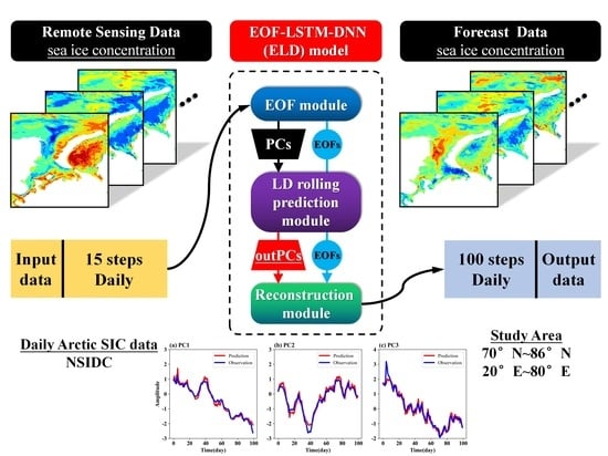
Considering the above, we develop a hybrid deep learning prediction model for the Arctic SIC based on the empirical orthogonal function (EOF) analysis, LSTM, and DNN, which is called the EOF–LSTM–DNN (ELD) prediction model in this study. By using EOF analysis, the spatio-temporal prediction problem of the SIC field can be transformed into a time-series prediction problem; then, we use the classical encoder–decoder architecture to process these time series. In this model, the LSTM neural network is used to encode the time series, and a fully connected DNN is used to decode the time series. Based on the above model, we can achieve an SIC prediction with a forecast window of 100 days in a rolling forecast method.

The rest of the paper is organized as follows: Section 2 describes the dataset used in this study. Section 3 introduces the theoretical frameworks of EOF, LSTM, and DNN, respectively. In Section 4, the sea ice concentration forecast experiments using the EOF–LSTM–DNN (ELD) model in the Arctic are presented in detail. Then, some discussions and future research suggestions are given in Section 5. Finally, in Section 6, we draw conclusions.

2. Study Area and Data

To date, the main institutions that release daily real-time sea ice concentration data products are the National Snow and Ice Data Center (NSIDC) and the University of Bremen in Germany. In this study, we used the daily Arctic sea ice concentration remote sensing data from the NSIDC for model construction and validation, which can be obtained from the following website: https://nsidc.org/data/seaice_index/ (accessed on 27 August 2021). This dataset is based on the passive microwave remote sensing inversions of three sensors (SMMR, SSM/I, and SSMI/S).

The spatial resolution of these gridded daily SIC products was 12.5 km. As shown in Figure 1, to fully reflect the strong sensitivity of the prediction model in capturing the fine spatial evolution in this study, we selected the region with more active spatial feature variations in the Arctic region as the study area. The latitude and longitude of the study area ranged from 70°N to 86°N and 20°E to 80°E, respectively.

Given the availability of the SIC dataset described above, we selected the daily SIC data from 1 January 1989 to 31 December 2019 for the construction and validation of the prediction model. One part of the SIC dataset from 1 January 1989 to 31 December 2016 was served as the training dataset, and the other part of the SIC dataset from 1 January 2017 to 31 December 2019 was served as the validation.

3. Methodology

The mid- and long-term evolutions of SIC is a spatio-temporal variation process. If we treat the evolutionary process of SIC as a time-series evolutionary problem, the spatial evolution characteristics are often lost because the spatial correlation is not considered. Similarly, if we only focus on the changes in spatial structure without considering the effects of temporal changes, this will make predictions impossible to achieve over a longer time scale. Therefore, it is necessary for us to consider both the spatial and temporal evolution of SIC to achieve better predictions.

As a classic “weapon” for spatio-temporal data mining and dimensional compression in the field of geosciences, EOF analysis can effectively extract the spatial features and temporal variations of research objects. As an enhanced version of the traditional regression neural network (RNN) model, LSTM can extract features from time series. In addition, DNN with a multilayer structure can decode the features extracted by LSTM well to obtain the final result of the SIC prediction. The combination of the above three techniques provides a reasonable method for the analysis and prediction of spatio-temporal fields. Therefore, we proposed an EOF–LSTM–DNN model for predicting the SIC, which is referred to as the ELD model in this study.

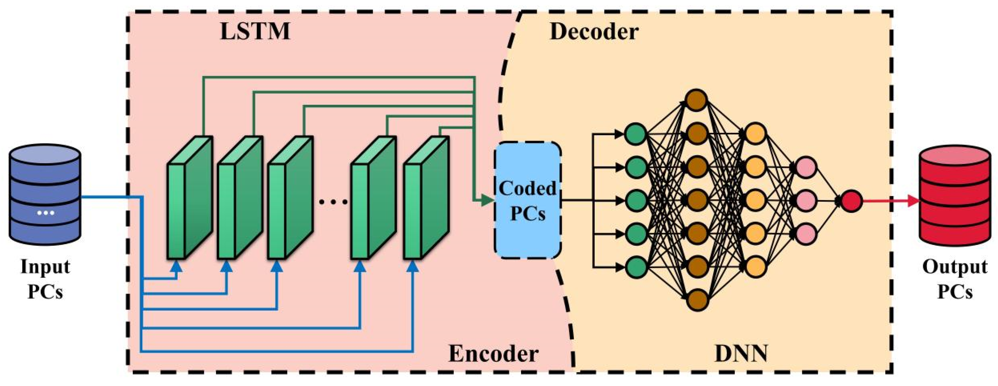
3.1. The Architecture of the ELD Model

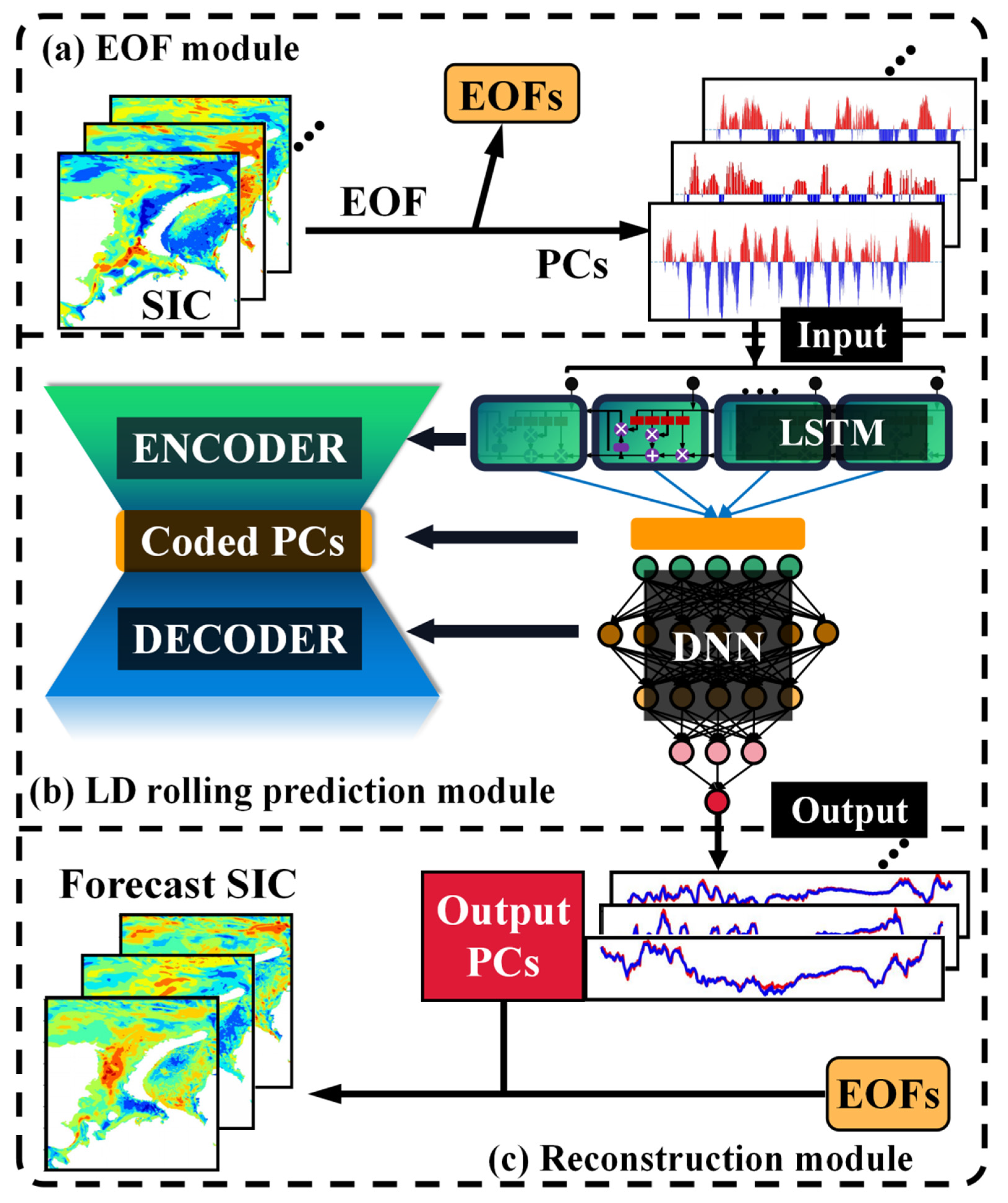
The ELD model is composed of three parts, namely, the EOF module, the LSTM–DNN (LD) rolling prediction module, and the reconstruction module, as shown in Figure 2. The functions of each module are described as follows:

First, in the EOF module, the original SIC satellite remote sensing dataset was divided into training and validation datasets. The training dataset can be decomposed into orthogonal spatial modes (EOFs) and corresponding principle components (PCs) by EOF analysis; then, the PCs of the validation dataset were obtained by projecting the testing set onto the EOFs obtained above. The details and related algorithm of the EOF decomposition are described in Section 3.2.

Next, in the LD rolling prediction module, a LSTM neural network was used to encode the input PCs, and then a multilayer deep neural network (DNN) was used to decode the encoded PCs to derive the future single-step prediction results. After the single-step prediction was completed, the model integrated the single-step prediction results with the original input to obtain a new input, and used the new input for the next prediction. The above steps were cycled several times to produce the final mid- and long-term prediction results for the PCs. Detailed information about the LSTM–DNN network is explained in Section 3.3.

Finally, the reconstruction module the SIC prediction field can be reconstructed by combining the output PCs in the LD rolling module with the EOFs obtained in the EOF module.

3.2. Empirical Orthogonal Function (EOF) Analysis

EOF decomposition was proposed by Pearson and introduced into the analysis of meteorological problems by Lorenz, which is commonly used to analyze variables [30,31]. It is often used to analyze the characteristics of the temporal and spatial distributions of the field and to separate the temporal and spatial characteristics of the variable field. Thus, the main information of the variable field can be represented by a few typical eigenvectors.

Before conducting EOF analysis, we need to remove the climatology to obtain the anomaly matrix ${\mathbf{X}}_{m\times n}$:

$${\mathbf{X}}_{m\times n}=\left[\begin{array}{cccccc}{x}_{11}& x_{12}& \dots & x_{1j}& \dots & x_{1n}\\ x_{21}& x_{22}& \dots & x_{2j}& \dots & x_{2n}\\ \dots & \dots & & \dots & & \dots \\ x_{i1}& x_{i2}& \dots & x_{ij}& \dots & x_{in}\\ \dots & \dots & & \dots & & \dots \\ x_{m1}& x_{m2}& \dots & x_{mj}& \dots & x_{mn}\end{array}\right]$$

(1)

In the above matrix, $m$ is the number of space observation points, $n$ is the length of the time series, and $x_{ij}$ represents the observation value of the $i\mathbf{th}$ spatial point on the $j\mathbf{th}$ day. Then, the covariance matrix ${\mathbf{C}}_{m\times m}$ of matrix ${\mathbf{X}}_{m\times n}$ can be calculated as:

$${\mathbf{C}}_{m\times m}=\frac{1}{n}{\mathbf{X}}_{m\times n}\times {\mathbf{X}}_{m\times n}^T$$

(2)

The eigenvalues $\left({\mathsf{\lambda }}_1,\dots ,{\mathsf{\lambda }}_m\right)$ and eigenvectors ${\mathbf{V}}_{m\times m}$ of ${\mathbf{C}}_{m\times m}$ can be expressed as follows:

$${\mathbf{C}}_{m\times m}\times {\mathbf{V}}_{m\times m}={\mathbf{V}}_{m\times m}\times {\mathsf{\Lambda }}_{m\times m}$$

(3)

$${\mathsf{\Lambda }}_{m\times m}=\mathrm{diag}({\mathsf{\lambda }}_1,\dots ,{\mathsf{\lambda }}_m)$$

(4)

where ${\mathsf{\lambda }}_i\left(i=1,2,\dots ,m\right)$ are arranged in descending order. Each non-zero eigenvalue corresponds to a column of eigenvectors, also referred to as the spatial pattern. For example, the eigenvector corresponding to ${\mathsf{\lambda }}_1$ is called the first spatial pattern (i.e., the first column of ${\mathbf{V}}_{m\times m}$) and so on. The spatial patterns are projected onto the matrix ${\mathbf{X}}_{m\times n}$ to obtain the PCs corresponding to the eigenvector:

$${\mathbf{PC}}_{m\times n}={\mathbf{V}}_{m\times m}^T\times {\mathbf{X}}_{m\times n}$$

(5)

The data of each row in the ${\mathbf{PC}}_{m\times n}$ corresponds to the PCs of each column of eigenvectors. The PC of the first spatial pattern corresponds to the first row of ${\mathbf{PC}}_{m\times n}$, and so on.

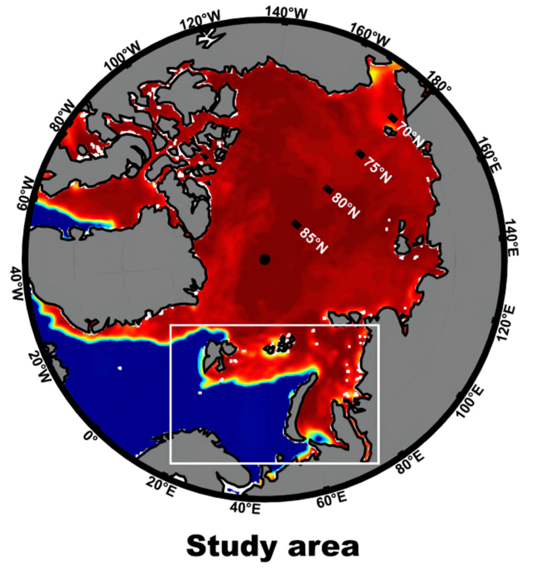
By the EOF analysis, the training datasets of the Arctic SIC are decomposed into EOFs and corresponding PCs. Here, we retain 15 EOFs with a total variance of 92%. Then, the validation dataset is project onto these 15 EOFs to obtain the PCs of the validation dataset. To date, what we need to consider further is how to better analyze and predict these time series (PCs).

3.3. Long Short-Term Memory Network (LSTM) and Deep Neural Network (DNN)

The LSTM network, a variant of RNN, was originally proposed by Hochreiter and Schmidhuber [32], and it is a solution to the vanishing and exploding gradient problem of RNNs. The core of RNN lies in its feature extraction and memorability (sharing of parameters within neurons). The neurons of the traditional RNN contain self-feedback connections, and the output is jointly determined by the input and the previous output, making it capable of remembering information. However, as the time interval increases, information is lost during the flow of neurons by multiplying the decimal points multiple times, resulting in the disappearance of the gradient. The influence of the current output on the subsequent output weakens until it disappears. Therefore, useful information cannot be continuously remembered. LSTM can continuously cycle the information to ensure the storage of information and remember the long-term information of the time series for future predictions. As the data flow though the network, the information can be stored, deleted, and added according to whether it is needed or not, effectively coping with the problem of vanishing gradients [33]. Therefore, LSTM can predict longer sequences and sequences with longer intervals. LSTM has advantages in time-series modeling with strong learning and generalization abilities, and has a good predictive effect on nonstationary data. When it learns the nonlinear features of a sequence, the high-dimensional mapping and evolution of the features does not only depend on the current independent information, but is also determined by the long-term influence mechanism that occurred historically and the current state. It is important to note here that the long-term historical information is actually the default behavior of the LSTM network structure rather than the result of human intervention or deliberate learning, which provides a good objective condition for future integrations with EOF analysis.

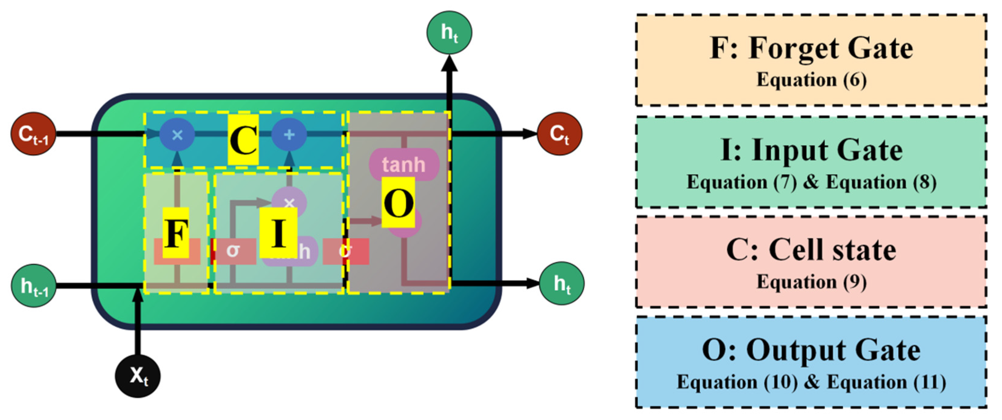
The LSTM is able to combine information learned in the long- and short-terms because its internal feature-processing mechanism is well able to control the unit states, processing, and mining mapping relationships through the information contained in the data itself. This capability is given by a structure called ‘gates’, as shown in Figure 3. These gate units that process and mine the input information realize the long-term learning capability of LSTM. The structure and the process of LSTM is as follows:

$$F_t=\sigma (W_f\cdot [h_{t-1},X_t]+b_f)$$

(6)

$$I_t=\sigma (W_i\cdot [h_{t-1},X_t]+b_i)$$

(7)

$$C_t^{\prime }=\tan h(W_C\cdot [h_{t-1},X_t]+b_C)$$

(8)

$$C_t=F_f\cdot C_{t-1}+I_t\cdot C_t^{\prime }$$

(9)

$$O_t=\sigma (W_O\cdot [h_{t-1},X_t]+b_O)$$

(10)

$$h_t=O_t\cdot \tan h(C_t)$$

(11)

where $\sigma$ is the sigmoid function; $W_f$, $W_i$, $W_C$, and $W_O$ are the weights applied to the concentration of the new input $X_t$ and the output $h_{t-1}$ from the previous cell; and $b_f$, $b_i$, $b_C$, and $b_O$ are the corresponding biases.

DNN is a multilayer feedforward network trained by error back-propagation. It takes the square of the network error as the cost function and uses the gradient descent method to calculate the minimum value of the cost function. The DNN model used in this study, which is presented in Figure 4, consists of five layers: an input layer, three hidden layers, and an output layer. Since there was no accurate rule to determine the number of neurons in the hidden layer, it was generally determined by repeated trial and error. After constantly trying different numbers of neurons during the operation of the model, the number was finally determined to be 41. The input layer consisted of 15 neurons, the number of neurons in the three hidden layers were 10, 10, and 5, and the output layer was 1.

4. Experiment Setup and Results

4.1. Experiment Setup

During the model training process, to make the training results converge more rapidly, we needed to initialize several hyper-parameters of the model. The learning rate (lr) was initialized to 0.0001, epoch was initialized to 200, batch size was initialized to 50, and dropout was initialized to 0.3. In our experiments, we performed the global optimization of the model using the Adam [34] algorithm, and used the mean squared error (MSE) as the evaluation metric for each training round to minimize the loss on the training dataset. To facilitate the experiments, the training dataset was constructed as a tensor of several small samples, where each individual sample contained a string of features for the input (15 steps) and a string of labels corresponding to the model output (100 steps). The output process of the model was divided into two steps: The first step was to directly output the prediction results for 1 time step; the second step was to input the results of 1 time step from the first step into the model as new features for rolling predictions until a total of 100 time steps were completed. Both of these steps were performed within the model. The MSE calculation of the output results and the inverse optimization of the model parameters were also performed in the above two steps. In this process, the MSE is calculated as follows:

$$MSE=\frac{1}{M}{\displaystyle \sum _{i=1}^M{({True}_i-{Predict}_i)}^2}$$

(12)

where $M$ is the number of the training samples; ${True}_i$ and ${Predict}_i$ represent the observation value and the predicted value for the $i\mathbf{th}$ sample, respectively.

4.2. Model Evaluation

To further evaluate the prediction performance of the ELD model, we compared it to a variety of machine learning models and existing numerical models. Here, root-mean-square error (RMSE), Pearson correlation coefficient (PCC), anomaly correlation coefficient (ACC), and mean absolute error (MAE) were used to verify the forecasting ability of different models. The equations used to calculate these performance metrics are as follows:

$$RMSE=\sqrt{\frac{1}{N}{\displaystyle \sum _{i=1}^N{({True}_i-{Predict}_i)}^2}}$$

(13)

$$PCC=\frac{{\displaystyle \sum _{i=1}^N({True}_i-\overline{True})({Predict}_i-\overline{Predict})}}{\sqrt{{\displaystyle \sum _{i=1}^N{({True}_i-\overline{True})}^2{\displaystyle \sum _{i=1}^N{({Predict}_i-\overline{Predict})}^2}}}},\left(\overline{True}=\frac{1}{N}{\displaystyle \sum _{i=1}^N{True}_i},\overline{Predict}=\frac{1}{N}{\displaystyle \sum _{i=1}^N{Predict}_i}\right)$$

(14)

$$ACC=\frac{1}{MM}\left\{{\displaystyle \sum _{\mathrm{j}=1}^{MM}\left[\frac{{\displaystyle \sum _{i=1}^N({AT}_{ij}-\overline{{AT}_j}\left)\right({AP}_{ij}-\overline{{AP}_j})}}{\sqrt{{\displaystyle \sum _{i=1}^N{({AT}_{ij}-\overline{{AT}_j})}^2{\displaystyle \sum _{i=1}^N{({AP}_{ij}-\overline{{AP}_j})}^2}}}}\right]}\right\},\left(\overline{{AT}_j}=\frac{1}{N}{\displaystyle \sum _{i=1}^N{AT}_{ij}},\overline{{AP}_j}=\frac{1}{N}{\displaystyle \sum _{i=1}^N{AP}_{ij}}\right)$$

(15)

$$MAE=\frac{1}{N}{\displaystyle \sum _{i=1}^N\left|{True}_i-{Predict}_i\right|}$$

(16)

$$SS=1-\frac{MSE(Predict,True)}{MSE(Reference,True)}$$

(17)

where $N$ is the number of testing samples, $MM$ is the number of spatial grid points, $Tru{e}_i$ and $Predic{t}_i$ represent the observation and predicted values for the $i\mathbf{th}$ sample, AT (anomaly true) and AP (anomaly prediction) represent the actual and predicted values after deducting climatic states, and $Reference$ is the comparison reference field. In addition, when SS > 0, it means the prediction result is better than the reference field; when SS = 1, it means error-free prediction; and SS < 0 means the prediction result is worse than the reference field.

4.3. Prediction Performance of the Principle Components

In this section, we take the satellite remote sensing of SIC as the observational value and perform the forecast experiment. The purpose of this section is to analyze the error source of the ELD model in the long-term SIC prediction process, as well as to analyze the ability of the ELD model to capture the different temporal evolution scales of Arctic sea ice concentration from the perspective of time series (PCs). In particular, the changes in monthly and seasonal scales are noteworthy.

At the beginning, we validated the proposed prediction model by evaluating the predictive performance of the time series. In evaluating the prediction trends over 100 days, we compared only the variation trend between the start and end moments of the forecast results of time series (PCs). Although such a comparison cannot capture the details of the forecast trends for all individual time steps within 100 days, it is still a valid way to measure the effectiveness of long-term time-series forecasts. Here, we used the validation dataset from 2017 to 2019 to conduct the prediction experiment on PCs, and then the prediction trend could be obtained by subtracting the first results from the 100th. As shown in Figure 5, the ordinate represents the change trend of the 100th day relative to the first day, with positive values representing the increase trend and negative value representing the decrease trend. The results of PC1 to PC3 in this figure show that the prediction trend of the ELD model matches the observational data very well. The RMSEs of the predicted trends for PC1, PC2, and PC3 were 0.018, 0.015, and 0.011, respectively.

The low RMSE of the forecast trend directly demonstrated the excellent long-term forecasting ability of the ELD model for each individual time series (PCs). However, it could effectively reflect the prediction performance of the ELD model on a smaller time scale. Therefore, we intercepted a set of prediction results to analyze the performance from the monthly scale to the seasonal scale. Figure 6 shows a comparison of the predicted PC1 to PC3 with the observational value for a total of 100 days from 1 March to 9 May 2019. As shown in Figure 6a, in the observational series, PC1 shows a decreasing trend from the 40th to 50th days, which contrasts with the trend from the 30th to 40th days. Fortunately, the predicted trend of the ELD model largely matches the trend of the observational series. It is easy to observe from Figure 6 that the ELD model performs well in capturing the overall trend at seasonal and monthly scales. Additionally, from Figure 6, we can observe that the small-scale signal fluctuations of about 10 days can be captured by this ELD model, which indicates its ability to predict multi-scale signals.

To investigate the advantages of the ELD model over the other artificial intelligence models in more depth, we designed a comparison experiment in the same experimental setting. Here, we chose a variety of classical machine learning models widely used in the field of time-series forecasting to compare to the ELD model, including logistic regression (LgR), back-propagation neural network (BPNN), RNN, and LSTM. At the same time, we selected the months with significant seasonal variations in Arctic sea ice concentration for the comparison. This experimental setup of forecasting effects in different months can not only directly reflect the long-term forecasting ability of the ELD model compared with other models, but also effectively compares the forecasting performance of multiple models on different time scales (especially in the month scale).

Table 1. Comparison of forecasting capabilities of multiple models in test datasets (2019).

Methods		Comparison of Three Months for Three Principal Components
		April 2019			August 2019			October 2019
		PC1	PC2	PC3	PC1	PC2	PC3	PC1	PC2	PC3
RMSE	LgR	1.364	0.370	0.638	0.186	0.171	0.454	0.148	0.397	0.477
	BPNN	0.734	0.319	0.581	0.115	0.160	0.382	0.130	0.320	0.437
	RNN	0.685	0.209	0.551	0.130	0.218	0.339	0.264	0.357	0.300
	LSTM	0.710	0.201	0.437	0.146	0.194	0.233	0.258	0.293	0.223
	ELD	0.043	0.129	0.233	0.018	0.192	0.123	0.096	0.262	0.222
MAE	LgR	1.206	0.382	0.596	0.168	0.135	0.409	0.137	0.323	0.387
	BPNN	0.629	0.303	0.545	0.093	0.145	0.342	0.114	0.238	0.355
	RNN	0.568	0.177	0.526	0.128	0.202	0.315	0.229	0.329	0.266
	LSTM	0.577	0.166	0.419	0.141	0.122	0.218	0.127	0.244	0.177
	ELD	0.033	0.099	0.189	0.013	0.125	0.095	0.063	0.218	0.176

shows the comparison results of PC1–PC3 for April, August, and October 2019.

The results presented in Table 1 show that the ELD model has a good prediction performance compared to other machine learning and deep learning models. For example, for the PC1 forecasts in April, August, and October 2019, the RMSE and MAE of the ELD model are 0.043 and 0.033, respectively. Meanwhile, the RMSE of the original LSTM, RNN, BPNN, and LgR models are 0.710, 0.685, 0.734, and 1.364, respectively; the MAE of original LSTM, RNN, BPNN, and LgR models are 0.577, 0.568, 0.629, and 1.206, respectively. As observed in Table 1, the superiority of the ELD model also holds for PC2 and PC3. The experimental results show that both MAE and RMSE can directly reflect the prediction errors of different models on the same validation dataset. However, the square term in RMSE can amplify abnormal results, so the results of RMSE are generally greater than those of MAE. From the above, we can observe that ELD has the lowest prediction error in most cases. The ELD model also performs better and more consistently with the observational values than the other models in the very few forecast cases with high errors. Such results show that the ELD model has the greatest advantage and robustness compared to other models in forecasting tasks at different monthly scales. It is worth noting that the model with higher robustness has a higher practical value and better prediction effect in the operational forecasting application of SIC.

4.4. Predictions and Comparisons of Daily Sea Ice Concentration

The prediction effectiveness of the independent PC is directly related to the prediction accuracy of the sea ice concentration space field, so it is extremely important to fully verify the SIC prediction ability of the ELD model. As shown in the previous section, we evaluated the time-series prediction ability of the ELD model using RMSE and MAE. The evaluation results show that the ELD model outperforms other machine learning models in predicting PCs. Distinct from the time-series prediction results, the results of the SIC spatial field prediction better reflect the evolution of SIC in spatial and temporal terms. In this section, we combined the EOFs stored in the EOF module with the predicted PCs to obtain the 100-day spatial forecasts of the SIC. Here, we used RMSE and PCC to analyze the spatial error and spatial correlation coefficient of the ELD model in the 100-day forecast statistics. Meanwhile, two statistical indicators, RMSE and ACC, were used to measure the forecast performance of the ELD model and the two baseline models.

The RMSE and PCC in Figure 7 show that the forecasts of the ELD model perform very well over the 100-day forecast period. At the end of the 100-day forecast, the RMSE of the ELD model spatial field forecasts is less than 0.24, and the PCC is greater than 0.9. From the spatial distribution of RMSE and PCC in Figure 7, we can observe that the prediction error of the ELD model is relatively large and the correlation coefficient is relatively low in the region with higher SIC values above 80° N. This may be because there are more nonlinear factors controlling the SIC in this area, which leads to the difference between this area and other regions, but the results still have certain reference values.

Then, we used persistent model and optimal climate normal (OCN) methods to further evaluate the performance of the ELD model. The persistence forecast is a forecast baseline model that is widely used in atmospheric and oceanic forecasting. It treats the forecast value as equal to the current value and can be expressed as follows: $X(t+\Delta t)=X(t)$, where $X(t)$ is the current observational value and $X(t+\Delta t)$ is the forecast result at time $t+\Delta t$. The OCN method is also a baseline method for mid- and long-term forecasting, which uses several years of averaged historical data as the forecast for the next year [35]. In this experiment, we used the averaged result from 1989–2013 as the forecast result.

Here, RMSE, PCC, and ACC were used to evaluate the accuracy of the ELD model, persistence prediction, and OCN results. In this experiment, ACC was used to evaluate the prediction performance of the persistence and ELD models, and PCC and RMSE are used to evaluate the performance of the OCN method, persistence prediction, and the ELD model. As shown in Figure 8, over the 100-day forecast period, the RMSE of the ELD model is consistently lower than 0.2, while the PCC and ACC are consistently greater than 0.7. Taking the 100th day as an example, the RMSE, PCC, and ACC of the ELD model are 0.19, 0.77, and 0.74, respectively. Notably, the RMSE of the ELD model increases gently, and the PCC and ACC decrease slowly. In contrast, the RMSE of the persistent forecast has a greater increase, and its ACC is below 0.5 on day 20. The RMSE of the OCN result is relatively stable, remaining at around 0.8, but much larger than the result of the ELD model. The PCC of the OCN results is also relatively stable in the 100-day statistics, remaining at around 0.64. The PCC of the persistent forecast and the ELD model shows a decreasing trend with the forecast time, but the decay rate of the persistent forecast is obviously faster. It can be observed that the ELD model is better than the persistence prediction and OCN methods in the mid- and long-term predictions.

4.5. Case Study and Comparison with Hybrid Coordinate Ocean Model Result

In this section, a comparison of the SIC spatial field forecast results of the ELD model with satellite remote sensing observational data are shown in Figure 9. The 100-day samples in 2019 predicted by the ELD model are compared with the satellite remote sensing data. As shown in this figure, the ELD model captures the evolution of the SIC during the prediction window. In the eastern region (black box) from the 1st to the 30th day, the SIC data of satellite remote sensing and the results of the ELD model show a significant decrease trend, which indicates that the ELD model can predict the spatial evolution trend of SIC well. In the comparison experiments shown in Figure 9, errors between the forecast results of the ELD model and the remote sensing SIC field are inevitable (especially in the forecast after 70 days). There are two main sources of its errors: (1) In the EOF module, we only select 15 EOFs for the final reconstruction. From the previous sections, 15 EOFs can explain 92% of the information in the SIC field, but a part of the information is still directly filtered, which can lead to non-negligible errors; (2) the rolling forecast structure of the ELD model causes the error of each time step to accumulate in the next time step. The above two points together cause the final forecast error, but it can be observed from the statistical results in Section 4.4 that the forecast accuracy of the ELD model is still the best result in all comparative experiments.

In addition, the numerical model-based sea ice forecasting tool is currently the dominant forecasting scheme, and it is widely used in operational sea ice forecasting. Therefore, we compared the performance differences between the ELD and numerical forecast models. It is worth noting that the forecast horizon of HYCOM was 9 days, and we used the HYCOM numerical model forecast results of Arctic sea ice concentration from 4 April to 12 April 2021 (9 days in total) for the experiment.

HYCOM is limited by the numerical calculation of a complex partial differential equation system, which makes it difficult for the HYCOM numerical prediction model to perform daily long-term SIC predictions. Therefore, the main purpose of the comparison experiment in this section was to compare the prediction accuracy of the ELD model and HYCOM at the same time step. Figure 10 shows the truth field, ELD forecast results, and HYCOM results (https://www.hycom.org/hycom, accessed on 4 April 2021), from which it can be observed that the forecast results of the ELD model are in good agreement with the truth field, and the spatial field distribution pattern from days 1 to 9 has a consistent trend. However, the forecast results of HYCOM already show great differences from the real spatial field distribution on day 9, especially in the eastern part of this figure (black box).

Then, we used the HYCOM results as the reference field to calculate the forecast skill score (SS) [36] of the ELD model. As shown in Figure 11, the SS of the ELD model relative to the HYCOM forecasts are all greater than 0, and the average SS of 9 days is 0.7172. This part is only a single-forecast experiment, so there is no obvious trend in the results of the forecast skill scores, but the value of SS can also reflect the forecast performance of the ELD model. It can be observed from the forecast examples and the forecast skill that the ELD model outperforms the HYCOM forecast model.

5. Discussions

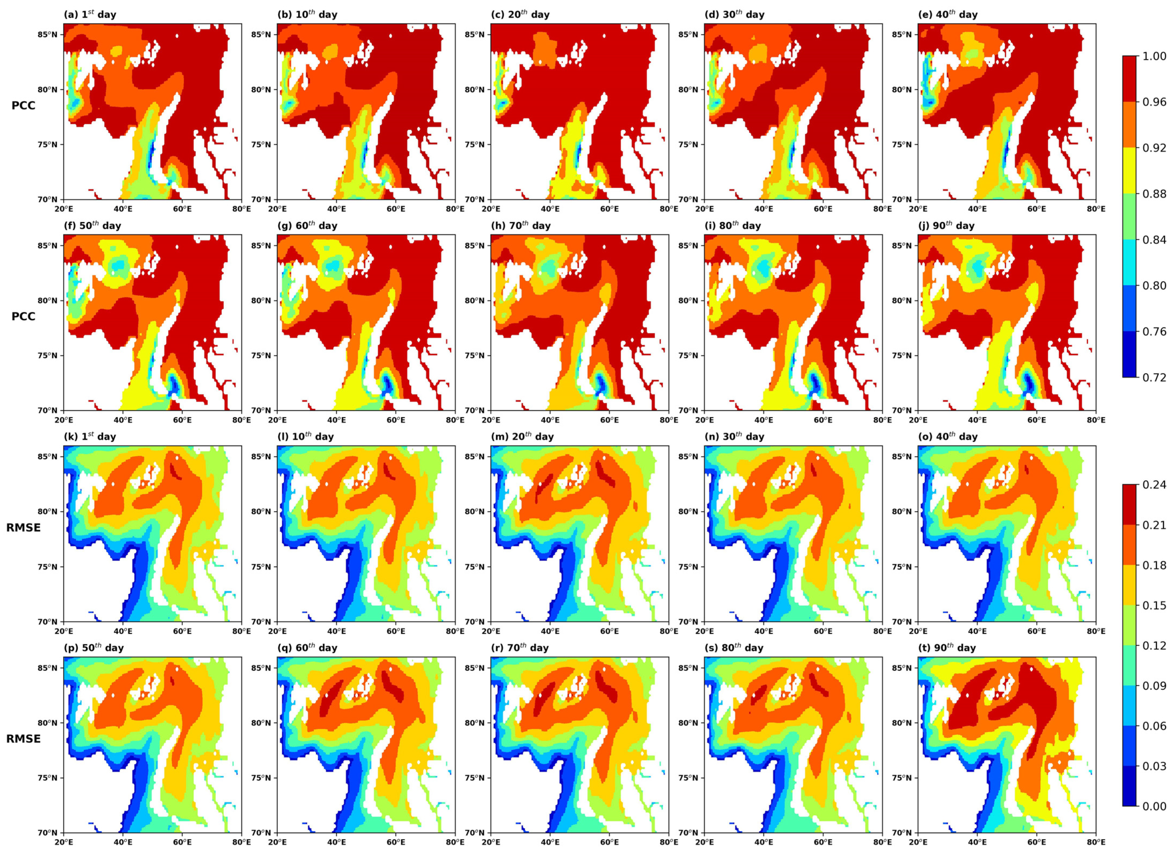
The ELD model makes full use of a large amount of satellite remote sensing SIC data to combine with the deep learning model. The forecast problem of the time–space field is transformed into the time series by the EOF method, which greatly simplifies the forecast difficulty and shortens the forecast time. Extensive experimental results confirm that the ELD model can obtain more accurate SIC 100-day prediction results at the expense of relatively short time consumption. The statistical results of the 100-day forecast of the ELD model show that the forecast RMSE increases with the forecast time. On the one hand, this is because the prediction error of the ELD model accumulates over time steps, which propagates the error from earlier time steps to later time steps, causing the long-term prediction results to be inferior to short-term results. However, the ELD model can effectively reduce the cumulative effect of this error, which is an important reason for its excellent performance in the 100-day forecast. On the other hand, medium- and long-term forecasting based on deep learning models may require sufficient training data and input data. At the same time, the quality of the data used for model learning is also a key factor in improving forecast timeliness. The pre-training of the ELD model is the most time-consuming stage in the whole experiment and the actual operational SIC forecast. The speed of EOF decomposition is slowed down due to the increase in the spatio-temporal resolution of the original data set. Although EOF is very time-consuming, its running results can be stored stably and can be directly called in subsequent prediction stages. It is worth mentioning that, when the dynamic mechanism is unclear or the solution of complex mathematical equations is difficult, the ELD model architecture scheme has wide applicability and flexibility for multi-domain spatio-temporal data mining and forecasting in the ocean and atmosphere.

The ELD model shows strong advantages in the current experimental stage, but we still found that it still had some aspects that could be improved. First, the ELD model has only been used for forecasting studies in a part of the Arctic. When the ELD model is used to study and forecast the entire Arctic region in the future, the computation load of the EOF module increases and the SIC prediction accuracy of the ELD model may decrease. If we want to produce mid- and long-term forecasts of high-resolution SIC in the entire Arctic region, the ELD model may need to be equipped with a high-performance computing platform, such as the GPU cluster. More importantly, the ELD model adopts the supervised learning method commonly used in deep learning. The label data used in the forecast training process greatly limit the forecasting ability of the ELD model to deal with sudden changes. In other words, the parameter results obtained by the ELD model training need to be retrained after having been used for a certain number of times, and need to pay more attention to data with abnormal changes in the SIC as much as possible. Such retraining is necessary to obtain more accurate prediction results. As we all know, the evolution process of SIC contains many dynamic and thermodynamic factors. In this experiment, we only conducted prediction research from the perspective of the SIC single variable, which ignored the influence of some necessary external factors on the evolution of SIC. This also provides new ideas for follow-up research. We can integrate multiple sea ice variables for forecasting, thereby improving forecast accuracy and forecast timeliness.

6. Conclusions

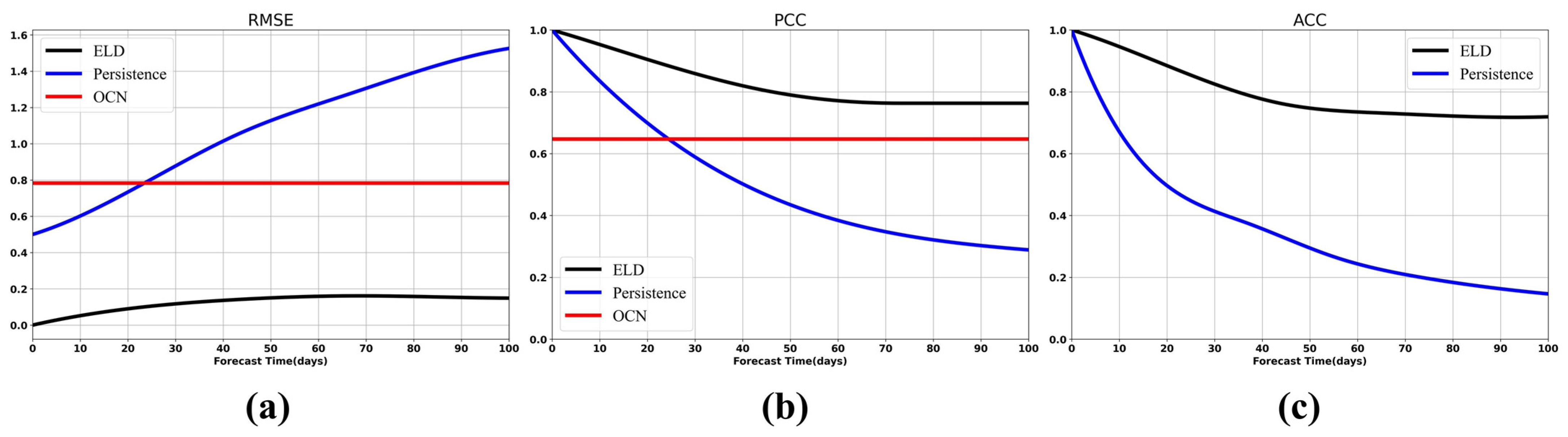
In this study, we proposed an Arctic sea ice concentration (SIC) forecast model (EOF–LSTM–DNN) based on statistical analysis and deep learning, and extend the effective forecast duration of SIC to 100 days. The model was driven by satellite remote sensing SIC data. The ELD model consisted of the empirical orthogonal function (EOF) method, long short-term memory network (LSTM), and deep neural network (DNN). Among them, EOF converts the spatio-temporal data of Arctic sea ice concentration into time series, LSTM encodes the historical time series, and DNN decodes the encoded information to obtain SIC forecast results. Meanwhile, we adopted the persistence prediction and optimal climatic normal (OCN) method as the baseline model to compare its RMSE, PCC, and ACC with the ELD model. The RMSE, PCC, and ACC of the ELD model at the 100th day of forecasts were 0.2, 0.77, and 0.74, respectively. While the RMSE of the persistence prediction and OCN results were 1.5 and 0.8, the ACC of the persistence prediction was 0.1, and the PCC of the persistence prediction and OCN results were 0.28 and 0.64. This shows that the ELD model is significantly better than the two baseline models mentioned above in mid- and long-term forecasting.

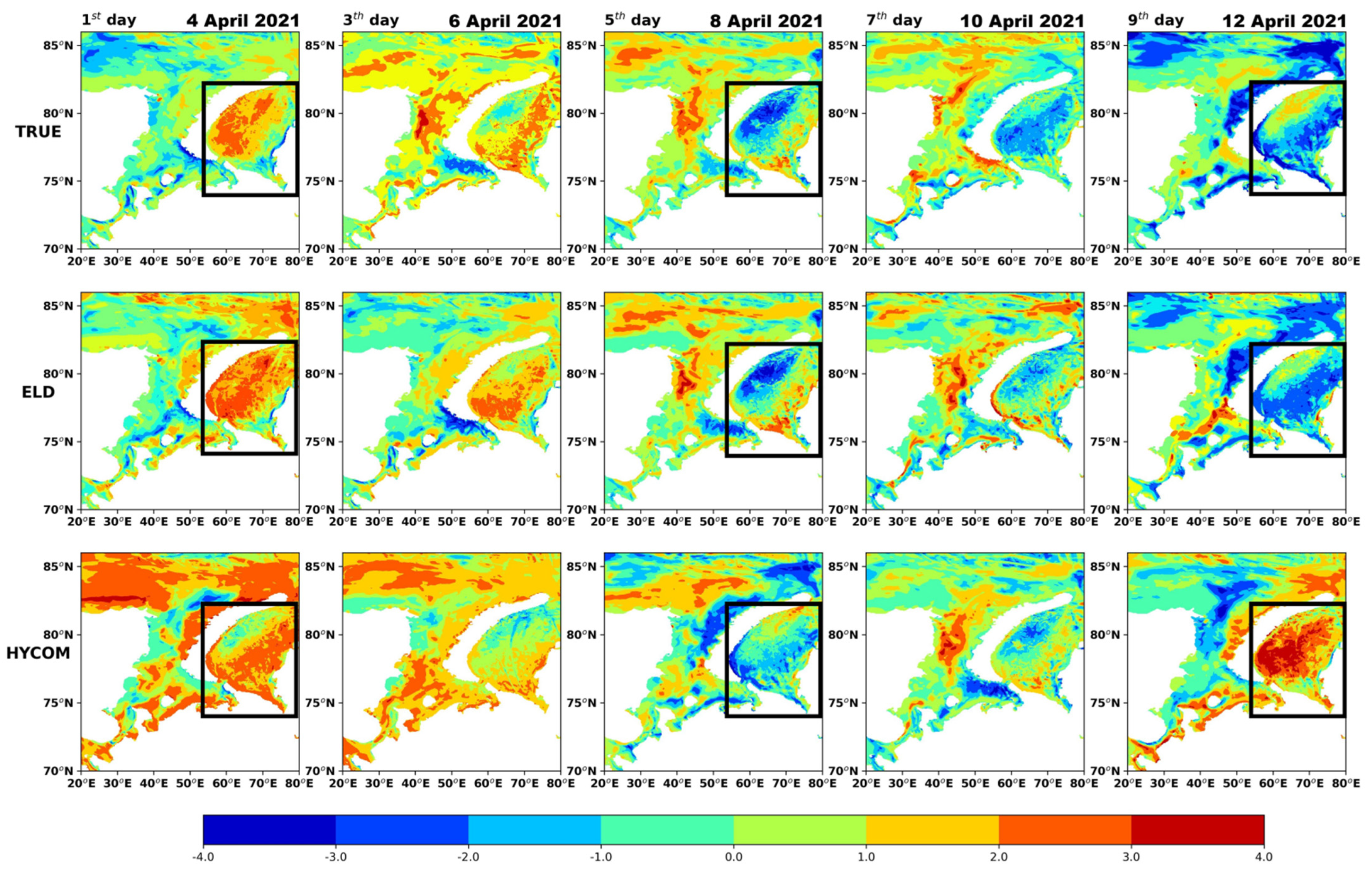
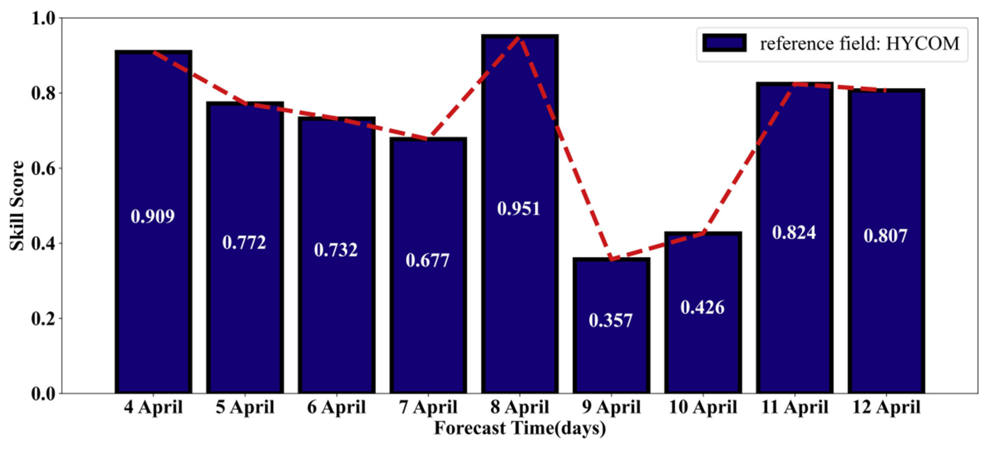
In comparison with the other machine learning models, the RMSE and MAE of the ELD model are significantly lower than those of logistic regression (LgR), back-propagation neural network (BPNN), recurrent neural network (RNN), and LSTM. At the same time, we compared the ELD model with the SIC results of the HYCOM numerical prediction. From the forecast skill score (SS), it can be observed that the SS of the ELD model relative to HYCOM is always greater than 0 (the average SS in 9 days is 0.7172), and the ELD model has obvious advantages in capturing the spatial evolution of SIC. The above experimental results all show that the ELD model has great potential in the mid- and long-term predictions of SIC.

References

1. Guemas, V.; Blanchard-Wrigglesworth, E.; Chevallier, M.; Day, J.J.; Déqué, M.; Doblas-Reyes, F.J.; Fuckar, N.S.; Germe, A.; Hawkins, E.; Keeley, S.; et al. A review on Arctic sea-ice predictability and prediction on seasonal to decadal time-scales. Q. J. R. Meteorol. Soc. 2016, 142, 546–561. [Google Scholar] [CrossRef]
2. Ledley, T.S. A Coupled Energy Balance Climate-Sea Ice Model: Impact of Sea Ice and Leads on Climate. J. Geophys. Res. 1988, 93, 15919–15932. [Google Scholar] [CrossRef]
3. Hwang, B.P.; Aksenov, Y.; Blockley, E.; Tsamados, M.; Brown, T.; Landy, J.; Stevens, D.; Wilkinson, J. Impacts of climate change on Arctic sea ice. MCCIP Sci. Rev. 2020, 2020, 208–227. [Google Scholar] [CrossRef]
4. Galley, R.J.; Key, E.; Barber, D.G.; Hwang, B.J.; Ehn, J.K. Spatial and temporal variability of sea ice in the southern Beaufort Sea and Amundsen Gulf: 1980–2004. J. Geophys. Res. 2008, 113, C05S95. [Google Scholar] [CrossRef]
5. Holland, M.M.; Stroeve, J. Changing seasonal sea ice predictor relationships in a changing Arctic climate. Geophys. Res. Lett. 2011, 38, L18501. [Google Scholar] [CrossRef] [Green Version]
6. Stroeve, J.; Hamilton, L.C.; Bitz, C.M.; Blanchard-Wrigglesworth, E. Predicting September sea ice: Ensemble skill of the SEARCH Sea Ice Outlook 2008–2013. Geophys. Res. Lett. 2014, 41, 2411–2418. [Google Scholar] [CrossRef] [Green Version]
7. Chi, J.; Kima, H.-C.; Leea, S.; Crawford, M.M. Deep learning based retrieval algorithm for Arctic sea ice concentration from AMSR2 passive microwave and MODIS optical data. Remote Sens. Environ. 2019, 231, 111204. [Google Scholar] [CrossRef]
8. Hunke, E.C.; Turner, A.K. Sea-ice models for climate study: Retrospective and new directions. J. Glaciol. 2010, 56, 1162–1172. [Google Scholar] [CrossRef] [Green Version]
9. Smith, G.C.; Roy, F.; Reszka, M.; Colan, D.S.; He, Z.; Deacu, D.; Belanger, J.-M.; Skachko, S.; Liu, Y.; Dupont, F.; et al. Sea ice forecast verification in the Canadian Global Ice Ocean Prediction System. Q. J. R. Meteorol. Soc. 2016, 142, 659–671. [Google Scholar] [CrossRef] [Green Version]
10. Barton, N.; Metzger, E.J.; Reynolds, C.A.; Ruston, B.; Rowley, C.; Smedstad, O.M.; Ridout, J.A.; Wallcraft, A.; Frolov, S.; Hogan, P.; et al. The Navy’s Earth System Prediction Capability: A New Global Coupled Atmosphere-Ocean-Sea Ice Prediction System Designed for Daily to Subseasonal Forecasting. Earth Space Sci. 2021, 8, e2020EA001199. [Google Scholar] [CrossRef]
11. Posey, P.G.; Metzger, E.J.; Wallcraft, A.J.; Hebert, D.A.; Allard, R.A.; Smedstad, O.M.; Phelps, M.W.; Fetterer, F.; Stewart, J.S.; Meier, W.N.; et al. Improving Arctic sea ice edge forecasts by assimilating high horizontal resolution sea ice concentration data into the US Navy’s ice forecast systems. Cryophere 2015, 9, 1735–1745. [Google Scholar] [CrossRef] [Green Version]
12. Sakov, P.; Counillon, F.; Bertino, L.; Lisæter, K.A.; Oke, P.R.; Korablev, A. TOPAZ4: An ocean-sea ice data assimilation system for the North Atlantic and Arctic. Ocean. Sci. Discuss. 2012, 9, 1519–1575. [Google Scholar] [CrossRef] [Green Version]
13. Yang, Q.; Liu, J.; Zhanhai, Z.; Cuijuan, S.; Jianyong, X.; Ming, L.; Chunhua, L.; Jiechen, Z.; Lin, Z. Sensitivity of the Arctic sea ice concentration forecasts to different atmospheric forcing: A case study. Acta Oceanol. Sin. 2014, 33, 15–23. [Google Scholar] [CrossRef]
14. Lins, I.D.; Araujo, M.; Moura, M.C.; Silva, M.A.; Droguett, E.L. Prediction of sea surface temperature in the tropical Atlantic by support vector machines. Comput. Stat. Data Anal. 2013, 61, 187–198. [Google Scholar] [CrossRef]
15. Patil, K.; Deo, M.C. Prediction of daily sea surface temperature using efficient neural networks. Ocean Dyn. 2017, 67, 357–368. [Google Scholar] [CrossRef]
16. Patil, K.; Deo, M.C.; Ravichandran, M. Prediction of Sea Surface Temperature by Combining Numerical and Neural Techniques. J. Atmos. Ocean. Technol. 2016, 33, 1715–1726. [Google Scholar] [CrossRef]
17. Zhang, Q.; Wang, H.; Dong, J.; Zhong, G.; Sun, X. Prediction of Sea Surface Temperature Using Long Short-Term Memory. IEEE Geosci. Remote Sens. Lett. 2017, 14, 1745–1749. [Google Scholar] [CrossRef] [Green Version]
18. Zheng, G.; Li, X.; Zhang, R.-H.; Liu, B. Purely satellite data-driven deep learning forecast of comolicated tropical instability waves. Sci. Adv. 2020, 6, eaba1482. [Google Scholar] [CrossRef]
19. Xiao, C.; Chen, N.; Hu, C.; Wang, K.; Gong, J.; Chen, Z. Short and mid-term sea surface temperature prediction using time-series satellite data and LSTM-AdaBoost combination approach. Remote Sens. Environ. 2019, 233, 111358. [Google Scholar] [CrossRef]
20. Shao, Q.; Li, W.; Hou, G.C.; Han, G.J. Ocean Reanalysis Data-Driven Deep Learning Forecast for Sea Surface Multivariate in the South China Sea. Earth Space Sci. 2021, 8, e2020EA001558. [Google Scholar] [CrossRef]
21. Shao, Q.; Li, W.; Han, G.; Hou, G.; Liu, S.; Gong, Y.; Qu, P. A Deep Learning Model for Forecasting Sea Surface Height Anomalies and Temperatures in the South China Sea. J. Geophys. Res. Ocean. 2021, 126, e2021JC017515. [Google Scholar] [CrossRef]
22. Shao, Q.; Li, W.; Hou, G.C.; Han, G.J. Mid-Term Simultaneous Spatiotemporal Prediction of Sea Surface Height Anomaly and Sea Surface Temperature Using Satellite Data in the South China Sea. IEEE Geosci. Remote Sens. Lett. 2022, 19, 1501705. [Google Scholar] [CrossRef]
23. Yan, Q.; Huang, W. Sea Ice Sensing From GNSS-R Data Using Convolutional Neural Networks. IEEE Geosci. Remote Sens. Lett. 2018, 15, 1510–1514. [Google Scholar] [CrossRef]
24. Wang, L.; Scott, K.A.; Xu, L.; Clausi, D.A. Sea Ice Concentration Estimation During Melt from Dual-Pol SAR Scenes Using Deep Convolutional Neural Networks: A Case Study. IEEE Trans. Geosci. Remote Sens. 2016, 54, 4524–4533. [Google Scholar] [CrossRef]
25. Chi, J.; Kim, H.-c. Prediction of Arctic Sea Ice Concentration Using a Fully Data Driven Deep Neural Network. Remote Sens. 2017, 9, 1305. [Google Scholar] [CrossRef] [Green Version]
26. Wang, L.; Scott, K.A.; Clausi, D.A. Sea Ice Concentration Estimation during Freeze-Up from SAR Imagery Using a Convolutional Neural Network. Remote Sens. 2017, 9, 408. [Google Scholar] [CrossRef]
27. Choi, M.; Silva, L.W.A.D.; Yamaguchi, H. Artificial Neural Network for the Short-Term Prediction of Arctic Sea Ice Concentration. Remote Sens. 2019, 11, 1071. [Google Scholar] [CrossRef] [Green Version]
28. Kim, Y.J.; Kim, H.-C.; Han, D.; Lee, S.; Im, J. Prediction of monthly Arctic sea ice concentrations using satellite and reanalysis data based on convolutional neural networks. Cryosphere 2020, 14, 1083–1104. [Google Scholar] [CrossRef] [Green Version]
29. Liu, Q.; Zhang, R.; Wang, Y.; Yan, H.; Hong, M. Daily Prediction of the Arctic Sea Ice Concentration Using Reanalysis Data Based on a Convolutional LSTM Network. J. Mar. Sci. Eng. 2021, 9, 330. [Google Scholar] [CrossRef]
30. North, G.R.; Bell, T.L.; Cahalan, R.F.; Moeng, F.J. Sampling Errors in the Estimation of Empirical Orthogonal Functions. Mon. Weather. Rev. 1982, 110, 699–706. [Google Scholar] [CrossRef]
31. North, G.R. Empirical Orthogonal Functions and Normal Modes. J. Atmos. Sci. 1984, 41, 879–887. [Google Scholar] [CrossRef] [Green Version]
32. Hochreiter, S.; Schmidhuber, J. Long short-term memory. Neural Comput. 1997, 9, 1735–1780. [Google Scholar] [CrossRef] [PubMed]
33. Shi, B.; Bai, X.; Yao, C. An End-to-End Trainable Neural Network for Image-Based Sequence Recognition and Its Application to Scene Text Recognition. IEEE Trans. Pattern Anal Mach. Intell. 2017, 39, 2298–2304. [Google Scholar] [CrossRef] [PubMed] [Green Version]
34. Zhu, Y.; Iiduka, H. Unified Algorithm Framework for Nonconvex Stochastic Optimization in Deep Neural Networks. IEEE Access 2021, 9, 143807–143823. [Google Scholar] [CrossRef]
35. Huang, J.; Barnston, A.G. Long-Lead Seasonal Temperature Prediction Using Optimal Climate Normals. J. Clim. 1996, 9, 809–817. [Google Scholar] [CrossRef]
36. Tonani, M.; Pinardi, N.; Fratianni1, C.; Pistoia, J.; Dobricic, S.; Pensieri, S.; Alfonso, M.d.; Nittis, K. Mediterranean Forecasting System: Forecast and analysis assessment through skill scores. Ocean Sci. 2009, 5, 649–660. [Google Scholar] [CrossRef] [Green Version]
Figure 1. Study area in this study.
Remotesensing 14 02889 g001
Figure 2. The architecture of the ELD model.
Remotesensing 14 02889 g002
Figure 3. The original model structure and calculation formula of LSTM.
Remotesensing 14 02889 g003
Figure 4. The process of the LSTM–DNN model.
Remotesensing 14 02889 g004
Figure 5. Forecast trend (100th minus first) of PC1 to PC3 by EOF–LSTM–DNN model (red line) compared with the corresponding truth (blue line), also a partial magnified view of the comparison results between the 400th and 800th days.
Remotesensing 14 02889 g005
Figure 6. A snapshot of one of the 100 days (1 March to 9 May 2019) forecasting cycles produced by the ELD model (red line) and the truth principal component (PC1(a)–PC3(c)) (blue line).
Remotesensing 14 02889 g006
Figure 7. Spatial distribution of Pearson correlation coefficient (PCC) (aj) and root-mean-square error (RMSE) (kt) of sea ice concentration (SIC) for the EOF–LSTM–DNN model. Calculated from daily forecasts over a 100-day range for 2017–2019.
Remotesensing 14 02889 g007
Figure 8. Comparison of (a) RMSEs, (b) PCCs, and (c) ACCs from persistence, OCN forecasts, and EOF–LSTM–DNN (ELD) forecasts. Calculated from daily forecasts over a 100-day range for 2017–2019.
Remotesensing 14 02889 g008
Figure 9. Comparison of the SIC spatial field forecast results (aj) of the ELD model with satellite remote sensing observational data (kt), selected for 100 days in 2019 from 1 January to 10 April.
Remotesensing 14 02889 g009
Figure 10. Comparison of forecast results between ELD forecast model and HYCOM numerical forecast model, days 1 to 9 in 2021 from 4 April to 12 April.
Remotesensing 14 02889 g010
Figure 11. The ELD model forecasting skill score (in comparison to HYCOM forecasts).
Remotesensing 14 02889 g011