Abstract
Rapid and accurate mapping of winter wheat using remote sensing technology is essential for ensuring food security. Most of the existing studies have failed to fully characterize the phenological features of winter wheat in mapping, resulting in low classification accuracy. To this end, this study developed a new multiple phenological spectral feature (Mpsf) and then used the generated new features as input data for a one-class classifier (One-Class Support Vector Machine, OCSVM) to map winter wheat. The main steps in this work are as follows: (1) Identifying key phenological periods. The spectral indices temporal profiles of winter wheat (after cloud masking) were drawn separately using different spectral indices, and the key phenological periods of winter wheat were identified with a priori knowledge of phenology. (2) Composition for a new feature. Composited the spectral features of winter wheat for each key phenological period to generate a new feature. (3) Training using a one-class classifier. The new feature was put into OCSVM for training, and the final winter wheat mapping result in the Beijing region was obtained. The cost of this new winter wheat mapping method is low and the accuracy is high. To verify the accuracy of this study, we compared the Mpsf map with three kinds of reference data, and all of them got good results. In comparison, with ground truth samples from Sentinel-2, the total accuracy was overall higher than 97.9%. The relative error of the 2019 winter wheat mapping result was only 0.51%, compared with the data from the Beijing Bureau of Statistics. In comparison, with an up-to-date available winter wheat-mapping product for Beijing (spatial resolution: 30 m), the Mpsf map has significantly fewer misclassifications. To our knowledge, this study produced one of the highest accuracy winter wheat-mapping products in Beijing for 2018 and 2019 to date. In general, we hope that this work can promote the development of winter wheat mapping and provide a reference for sustainable agricultural development and governmental decision-making.
1. Introduction
Due to global climate change and the supply chain disruptions because of COVID-19, people pay extensive attention to food security [1]. As wheat is the most widely grown crop in the world [2], an accurate grasp of its cultivation area is essential for ensuring food security. Winter wheat is one of the most critical crops in Beijing, its acreage and spatial distribution data are the basis for the regional balance of grain and the comprehensive production capacity of agricultural resources. For the sustainable development of Beijing, timely and accurate acquisition of its winter wheat cultivation area is of great significance to optimize agricultural production management. Traditional acquisition of a winter wheat cultivation area relied on human field surveys, which are limited by manpower, material resources, and natural conditions. It is difficult to meet the current demand for rapid monitoring of winter wheat cultivation areas. Remote sensing technology can quickly, accurately, and objectively monitor changes in agricultural production and resource utilization, and has now become one of the important means to monitor the distribution of winter wheat. Mapping winter wheat using remote sensing technology is conducive to grasping agricultural information timely and assisting macro-control.
Remote sensing technology plays a unique role in monitoring winter wheat cultivation areas for in-depth observations in spatial and temporal respects [3]. Nowadays, the three main types of remote-sensing data sources for wheat mapping are: Synthetic Aperture Radar (SAR), the integration of SAR and optical data, and optical remote sensing. SAR can keep working in any weather and at any time. The technology of SAR captures small changes between crops and land, and the surface information of vegetation can be obtained through the penetration of radar satellites [4]. The downside is that the point scatterers contained in the pixels of radar data can cascade into interference and speckle, reducing the accuracy of the mapping [5]. In the extraction of winter wheat using SAR data, since SAR backscatter differs for different plant structures, the backscatter features in different periods were mainly studied to distinguish winter wheat from other crops [6]. However, due to the high overlapping responses of different crops, choosing the appropriate threshold separation method became a challenge, which directly affected the accuracy of the classification results. Previous studies suggested that the combination of optical-SAR integration data could improve winter wheat classification accuracy [7,8]. But the huge imaging difference between SAR and optical data makes it difficult to select an appropriate fusion method [9]. In view of the above-aforementioned limitations of SAR and optical-SAR integration data, the use of optical data is still the dominant trend in winter wheat mapping.
At present, in terms of spatial resolution, the methods for winter wheat mapping using optical data are mainly divided into three groups: very high-resolution data (less than 5 m), fine-resolution data (5–100 m), and medium-resolution data (100–1000 m) [10]. Very high-resolution data can reach the sub-meter level of remote sensing and obtain detailed ground object information, but its high costs limit the application of regional area winter wheat mapping [11,12]. Medium-resolution remote sensing data, represented by Medium Resolution Imaging Spectroradiometer (MODIS), have proven to be of good applicability in many winter wheat mapping studies [13,14,15]. However, because of its severe mixed pixel effect, it produced large misclassifications, and could not meet the requirements of winter wheat refinement extraction. Given the limitations mentioned above of very high-resolution and medium-resolution data, fine-resolution data provide a suitable solution for accurate winter wheat mapping at regional scales.
We can find excellent examples of winter wheat mapping at regional scales using fine-resolution data in many previous studies [16,17,18,19]. In paper [17], it applied Landsat and Sentinel data to map the early-season distribution of winter wheat in 11 Chinese provinces from 2016 to 2018. They used the time window from October to April to compare the similarity of monthly maximum composite NDVI between the collected sample and winter wheat by increasing month by month, so as to extract winter wheat, showing good performance in a large-scale mapping. However, it should be noted that a single phenology cannot represent all the spectral features of the growth stage for winter wheat. Moreover, when there is continuous extreme weather (e.g., prolonged rainfall, snowstorm, hail, fog) within a phenological period, few remote sensing images will be available, which may affect the accuracy of classification results.
Another issue in using phenological features to map winter wheat in fine-resolution images is the selection of vegetation index. In some previous studies, a single vegetation index temporal profile was used to identify winter wheat in multiple phenological periods [16,20,21]. Normalized Difference Vegetation Index (NDVI) was the vegetation index used in the mentioned studies, and its applicability as the most widely used vegetation extraction method at present is beyond doubt. However, if only a single NDVI time series data is used to extract the winter wheat area during the whole phenological period, the classification result will be affected if the spectral index temporal series data profile of other vegetations is similar to winter wheat [20]. To enhance the spectral separation between winter wheat and other vegetation, it is necessary to introduce different vegetation index combinations in multiple phenological periods to improve the accuracy of winter wheat mapping. Therefore, using multiple vegetation indices is the mainstream method of identifying crops in recent studies [22,23,24]. In study [23], it defined four key phenological periods of winter wheat in North China Plain based on the simulated Vegetation Index (VI) time series data. Paper [24] developed a vegetation index–phenological index (VI-PI) classifier to map the interannual change of maize planting area in the Hetao irrigation area of North China from 2003 to 2012.
Based on the above analysis, in order to fully characterize the phenological features of winter wheat in mapping, this study developed a new multiple phenological spectral feature (Mpsf) and then used the generated new features as input data for a one-class classifier (OCSVM) to map winter wheat. This new feature was based on the spectral characteristics of winter wheat in multiple phenological periods. Our objectives: (1) Develop a Mpsf map in the Google Earth Engine (GEE) to fully obtain phenological features in multiple key phenological periods for winter wheat. (2) Produce a high-precision winter wheat-mapping product for the Beijing area. Therefore, we hope that this work can promote the development of winter wheat mapping and provide a reference for sustainable agricultural development and governmental decision-making. The rest of this paper is organized as follows: Section 2 presents the materials and methods, which include the study area, data, and methods. Section 3 describes the results of the mapping and the classification accuracy assessment. Section 4 discusses the main achievements, limitations, and future work. Conclusions are given in Section 5.
2. Materials and Methods
2.1. Study Area
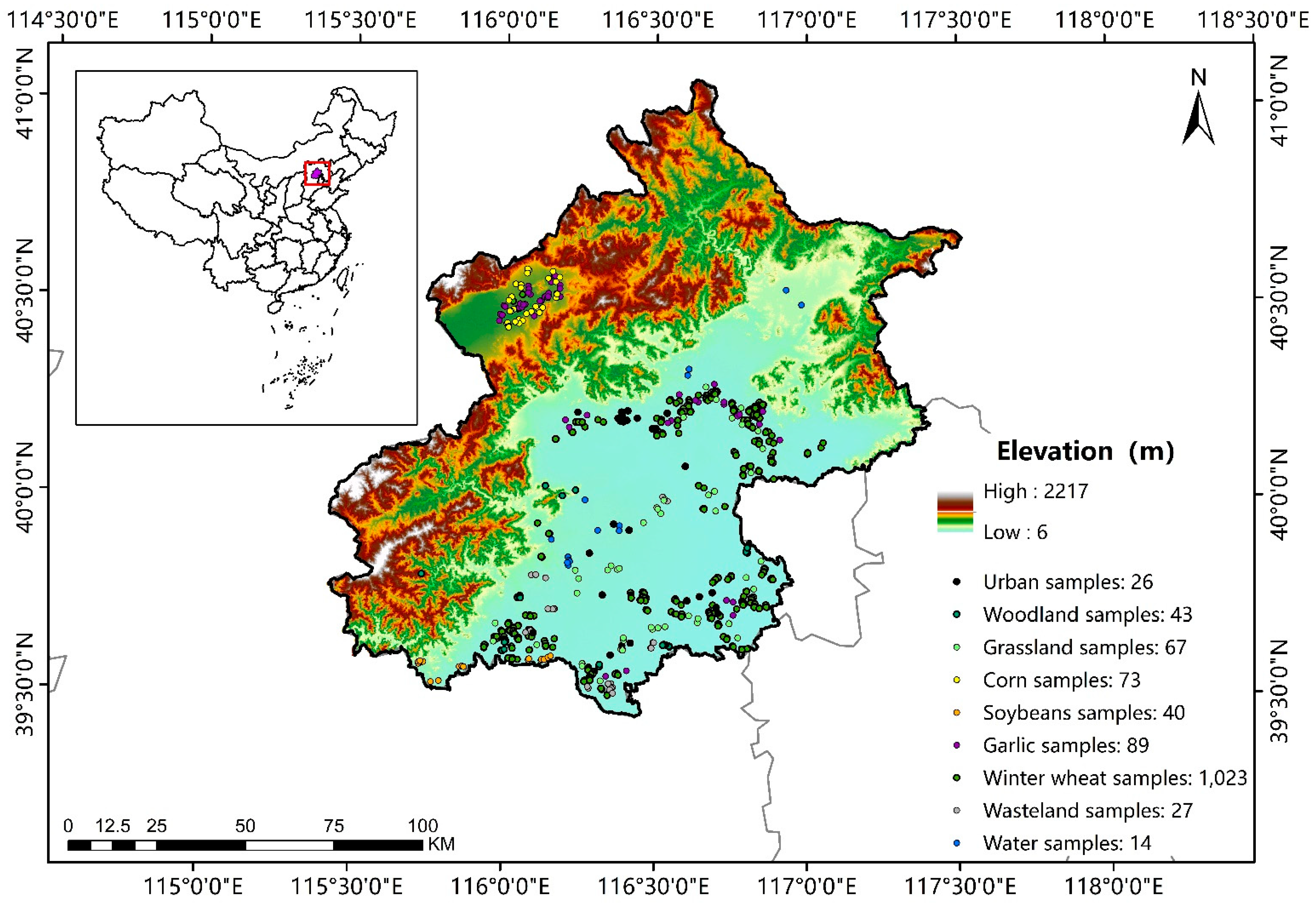
The study area of Beijing is located at the northern end of the North China Plain (39°28′–41°05′N, 115°24′–117°30′E), with the highest elevation of 2217 m and the lowest elevation of 6 m (Figure 1). Beijing is mountainous in the west and north, and plain in the southeast, belonging to the warm temperate semi-humid continental monsoon climate zone. According to the official data of the China Weather Website, the average annual temperature in Beijing’s plain areas is between 11 °C and 13 °C, in mountainous areas below 800 m above sea level it is between 9 °C and 11 °C, and in alpine areas, it is between 3 °C and 5 °C. The annual extreme maximum temperature is generally between 35~40 °C, and the annual extreme minimum temperature is generally between −14~−20 °C. The annual average precipitation is 430.9 mm, which is mainly concentrated in summer. Crops planted in Beijing mainly include winter wheat and corn, among which winter wheat is mainly distributed in plain areas and counties in the east and south of Beijing. Winter wheat in Beijing is usually sown from mid-to-late September to late October of the previous year, turning green in mid-March of the following year, flowering in early May, and harvesting around mid-June.
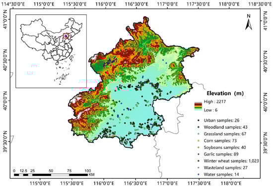
Figure 1.
Geographical location and DEM of Beijing (DEM: Digital Elevation Model, data provided by Shuttle Radar Topography Mission), and distribution map of classes samples that exist in study area. Specifically, a total of 1023 winter wheat samples with the area of 8,658,500 square meters were collected (selection of other classes can be seen in Section 2.2.2).
2.2. Datasets
2.2.1. Sentinel-2 Imagery
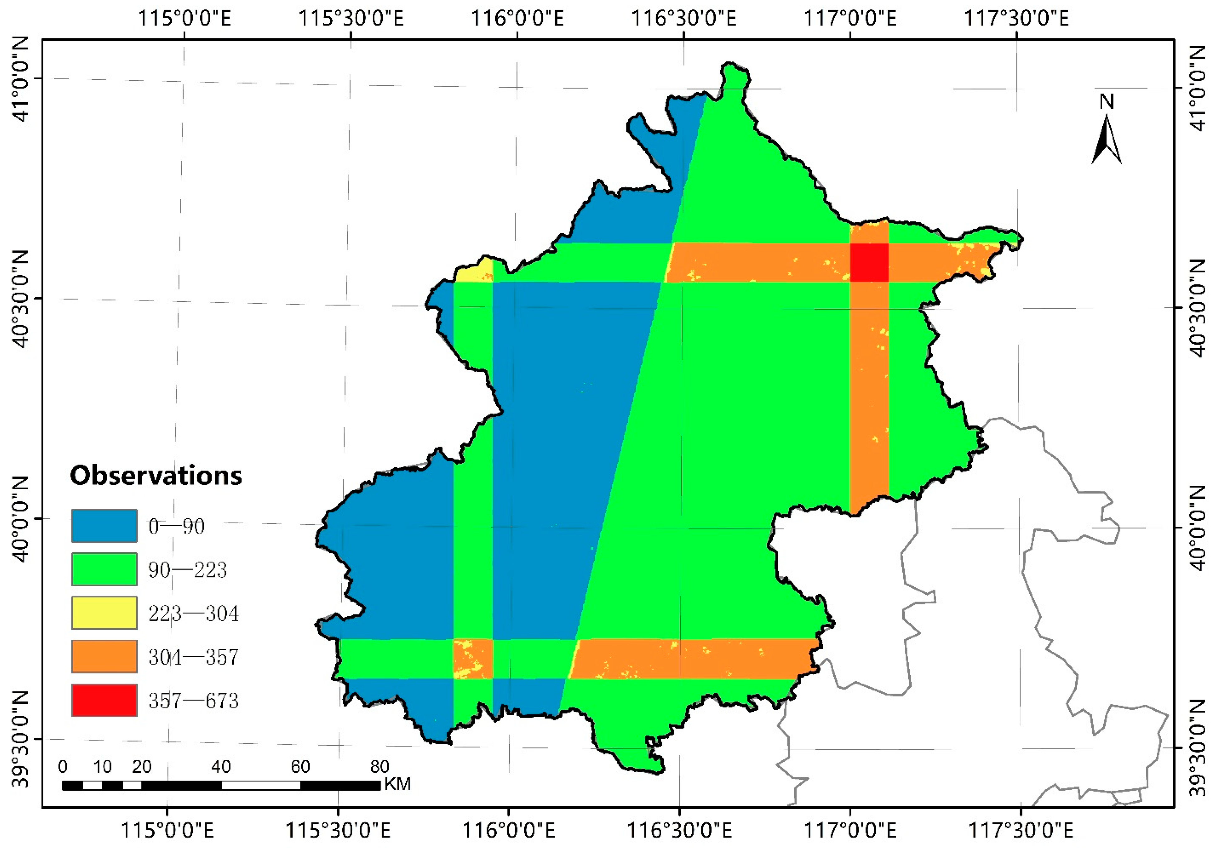
Based on the GEE cloud platform, in this study, we obtained a total of 1720 images of the Beijing region from September 2018 to July 2020 from Sentinel-2 surface reflectance dataset. The Sentinel-2 (S2) global revisit frequency is 5 days, the Multispectral Instrument (MSI) sampled 13 spectral bands: visible and near infrared at 10 m, red edge and SWIR at 20 m, and atmospheric bands at 60 m spatial resolution (illustrated in Google Earth Engine datasets). It provides data suitable for assessing the status and changes in vegetation, soil, and water cover. The surface reflectance dataset used in this work is Level-2A orthorectified. In order to exclude the possible influence of cloud and fog, etc., we filtered all Sentinel-2 images of the Beijing area in the time period (2018–2020) based on cloud percentage, and then applied cloud-free pixels to generate composite images containing rich phenological information. After cloud-percentage filtering, a total of 1235 images were actually applied to the subsequent operation. We counted the number of observations by the images used to the study area at the pixel level, as shown in Figure 2. According to the classification principle of Natural breaks (Jenks), the number of observations was divided into 5 categories. A number between 0 and 90 accounted for 64.68% of the total, and 90-223 accounted for 28.60%.

Figure 2.
The distribution of number of observations in the study area from 2018 to 2020 (after cloud masking).
2.2.2. Reference Data
In order to verify the feasibility and accuracy of the Mpsf winter wheat mapping method of the Beijing area, in this study, we introduced three types of reference data: a visual interpretation of winter wheat samples from very high-resolution images provided by Google Earth (GE), the official investigation of winter wheat provided by the Beijing Bureau of Statistics (BBS), and a winter wheat-mapping product with a spatial resolution of 30 m in Beijing area.
- (1)
- Visual interpreting of winter wheat samples. Due to the spread of COVID-19 and restrictions on epidemic prevention policies, we were unable to obtain the latest field survey data for the study area. Fortunately, Google Earth’s ability to provide very high-resolution data and historical images solved the limitation of lack of samples in the field. Some previous studies have proved that the very high-resolution imagery in GE is an effective data source to collect samples [25,26,27]. A total of 1158 ROIs, including 1023 winter wheat ROIs (155,853 pixels) and 135 non-winter wheat ROIs (389,848 pixels), were obtained through comparison and visual interpretation of multi-phenological images in the study area. Half of the winter wheat samples were used to train one-class classifiers, and the other half of the winter wheat samples and non-winter wheat samples were used to verify mapping accuracy. Non-winter wheat samples included non-vegetation types (e.g., urban (26 ROIs, 45,087 pixels), water (14 ROIs, 25,091 pixels), wasteland (27 ROIs, 46,780 pixels)), and other vegetation types (e.g., other crops (202 ROIs, 136,440 pixels), woodland (43 ROIs, 81,870 pixels), grassland (67 ROIs, 54,580 pixels)). Among the vegetation types, half were agricultural areas and the remaining half were woodland and grassland. The number of training and validation ROIs of the 11 districts that planted winter wheat in Beijing (ranking source: official data from BBS) are listed in Table 1. It should be noted that different ROIs consisted of different numbers of pixels. If samples were collected in a large area, with the same land cover type, it was easy to draw a complete polygon in GE, resulting in the number of ROIs being small, such as the sample selection of mountain areas (e.g., Pinggu, Huairou, Miyun, Yanqing), as well as urban areas (e.g., Haidian, Chaoyang).
 Table 1. Number of ROIs in 11 districts which planted winter wheat in Beijing.
 - (2)
- Winter wheat area statistics from the BBS. The planting area data of winter wheat in each district of Beijing can be accessed from the statistical yearbook published by the Beijing Bureau of Statistics (http://tjj.beijing.gov.cn/ (accessed on 24 July 2022)). Since statistical yearbooks generally report the data of the previous year in the later year, and winter wheat is harvested in the summer of the year after sowing in the autumn of the previous year, according to the time interval for winter wheat in our study (2018–2020), the statistical yearbooks of Beijing in 2019 and 2020 (published in 2020 and 2021, respectively) should be queried.
- (3)
- An open-source 30-m winter wheat-mapping product in the Beijing area. Paper [17] produced a 30-m mapping of the early-season winter wheat in 11 provinces in China, which is one of the most winter wheat-accurate mapping data available in Beijing region. Thus, it was selected as auxiliary data to verify the mapping accuracy for this work.
2.3. Methods
The winter wheat mapping method in this study mainly includes the following 2 steps: (1) The Mpsf was developed to construct a new feature combining 3 distinctive phenological periods (details in Section 2.3.1). (2) Input the Mpsf-based composite image to OCSVM for training, and the final winter wheat mapping result in the Beijing region was obtained. The parameter settings of OCSVM were explained in Section 2.3.3.
2.3.1. Multiple Phenological Spectral Feature (Mpsf) Composite Method
As shown in Figure 3, the method of Mpsf can be mainly divided into three steps: (1) We removed the clouds in Sentinel-2 images by two cloud masking methods at scene-level and pixel-level, respectively (Cloud Masking). (2) By analyzing the time profiles of six spectral indices, three key winter wheat phenological periods were determined (Identifying Key Phenological Periods). (3) Various spectral indices were calculated for each image collected in corresponding phenological periods. Then, we derived six composite images by the median composite method of spectral indices, corresponding to each phenological period. Finally, a new feature image was constructed by stacking the six indices composite images (Image Composite Method for New Feature Based on Key Phenological Periods).
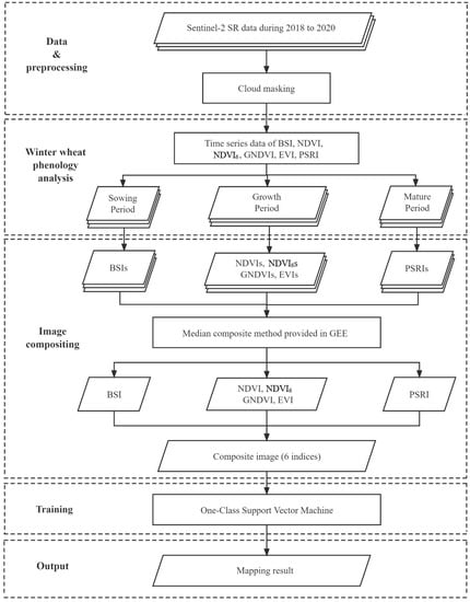
Figure 3.
Flowchart of winter wheat mapping method in this study.
Cloud Masking
The cloud masking methods were used to remove the cloud from the images that consisted of two dimensions: scene-level and pixel-level. Firstly, a parameter of 70% is set as the threshold for filtering the cloud-cover percentage. A Sentinel-2 image was excluded when its cloud percentage was greater than 70%, the setting of this parameter is based on previous studies [9,28,29]. After using the scene-level cloud removal method, the cloud pixels of the remaining images were filtered by a pixel-level method. The pixel-level cloud removal method is widely used in many cases and it’s officially provided by the GEE group for Sentinel-2 images. Specific pixel values in the QA60 band were selected to remove cloud pixels in low-cloud images [30].
Identifying Key Phenological Periods
In this step, six vegetation indices were introduced to highlight the spectral separation between winter wheat and other vegetation, and spectral indices temporal profiles of winter wheat samples were drawn based on three of them (Bare Soil Index (BSI), Normalized Difference Vegetation Index (NDVI), and Plant senescence reflectance Index (PSRI)) to classify 3 key phenological periods (sowing, growing, and mature periods). The reasons for selecting the three vegetation indices are as follows: (1) BSI was used to detect the sowing period, because at this stage (mid to late September to early October), land planted with winter wheat had a low vegetation coverage, while land covered by other vegetations had a high vegetation coverage. BSI has a strong ability to identify bare land [31]. (2) As a widely-used vegetation index, NDVI is very effective for analyzing vegetation dynamics in geographical areas [32], and many previous studies have used NDVI to extract winter wheat successfully [4,14,20,21,32,33]. (3) PSRI was proposed to measure the maturity of winter wheat. Since it is sensitive to carotenoids in senescent leaves [34], it is often used to determine the stages of a crop’s maturity with high accuracy [35].
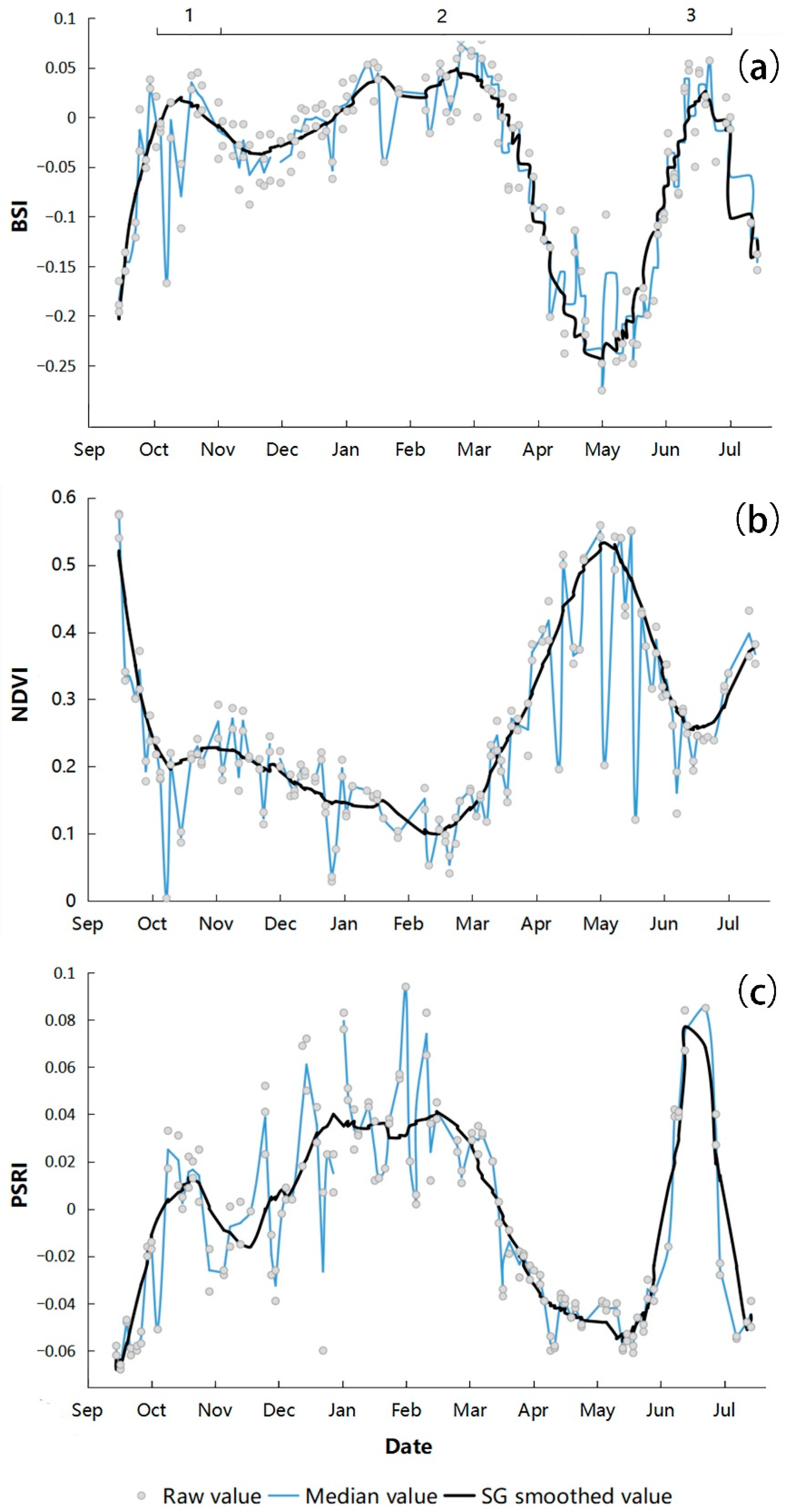
In order to draw accurate spectral indices temporal profiles of winter wheat, we used data from pure winter wheat pixels (150 ROIs, evenly distributed throughout the winter wheat field of the Beijing region) obtained from visual interpretation of very high-resolution images on Google Earth. For each pixel, 3 spectral indices temporal profiles were obtained by calculating BSI, NDVI, and PSRI vegetation indices. As shown in Figure 4, the data in the figure were calculated from all available Sentinel-2 images during the study time range (mid-September 2018 to mid-July 2020) after cloud masking. Grey dots represent the raw indices values, blue lines represent the median values of raw indices on the same day, and black lines are the raw values smoothed by the Savitzky-Golay (SG) filter [36]. In the parameter setting of the SG filter, we combined the actual situation and referred to the method in previous studies [9,33], and set the smoothing window as 10 and the degree of smoothing polynomial as 3.
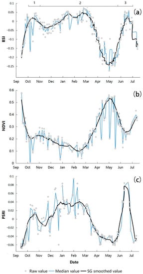
Figure 4.
Spectral indices temporal profiles of winter wheat samples (150 ROIs, evenly distributed throughout the winter wheat field of Beijing region). Subfigure (a–c) are BSI, NDVI, and PSRI, respectively. The digits above the time series profiles denote key phenological periods of winter wheat. 1: sowing (1 October to 31), 2: growth (1 November to 19 May), 3: mature (20 May to 30 June).
After analyzing the spectral indices temporal profiles of Figure 4, and considering the prior phenological knowledge of winter wheat, the following three key phenological periods were determined:
- (1)
- Sowing period. At this stage, the vegetation coverage of the land was low and soil signals emerged. In October, BSI showed a series of high values, while NDVI was at a low value, indicating that the land was not covered by obvious vegetation (Figure 4a).
- (2)
- Growth period. Before the overwintering period (from mid-December to late February of the following year), winter wheat grew slowly. After the overwintering period, winter wheat entered the stage of rapid growth, and its chlorophyll signal increased sharply and reached the peak of the whole phenological period, as shown in the spectral profile of NDVI (Figure 4b). In this period, the values of BSI and PSRI were at their nadir.
- (3)
- Mature period. From late May, winter wheat began to mature. At this time, chlorophyll content decreased sharply while carotenoids increased, and the corresponding spectral index changes were shown in Figure 4b,c. With the harvest of winter wheat, large areas of winter wheat fields were bare (soil signal appeared again), and at the same time, the value of BSI increased significantly (as shown in Figure 4a).
Image Composite Method for New Feature Based on Key Phenological Periods
In this step, we used the median composite method provided by GEE to compute the value of 6 indices (listed in Table 2) in each image, respectively, and finally took each processed image as a single band to stack a new feature image, so that the final image contained the information from three key phenological periods (mentioned in Section 2.3.2) of winter wheat. For example, in the BSI median composite method, all images after cloud masking in the study time range were calculated by BSI index, and then the median of all values was taken for construction, so as to obtain the single band of BSI. The indices used are BSI, NDVI, GNDVI, NDVI6, EVI, and PSRI. Among them, BSI was used in the sowing period, NDVI, GNDVI, NDVI6, and EVI were used in the growth period of winter wheat, and PSRI was used in the mature period.
Table 2.
Formulas of the selected spectral indices with the corresponding phenological periods.
The reasons for using the above six indices to construct a new multiple phenological spectral features for winter wheat are as follows: (1) As analyzed in Section 2.3.2 for BSI, NDVI, and PSRI, these three indices have significant abilities in identifying winter wheat during special phenological periods, so they were selected. (2) In addition, for the growth period of winter wheat, we introduced GNDVI, NDVI6, and EVI to complement NDVI. The winter wheat growth period spends most of its time in its whole phenological period, it can be further subdivided into the seedling stage, tillering stage, over-wintering stage, green returned stage, jointing stage, etc. Many previous studies [7,14,17,19,43,44] indicated that one of the key stages for extracting winter wheat is the growth period, so this period of winter wheat, in accurate identification, is the key to ensuring the mapping accuracy. We tried to use indices combinations to fully reflect the phenological features of winter wheat at this stage. With the change of environment, crop chlorophyll content will also change correspondingly, which has a good correlation with the value of SPAD (Soil and Plant Analyzer Development). In previous studies [45,46], the SPAD value can reflect the chlorophyll content of crop leaves, which is an important indicator to characterize the health status of crops. The multispectral vegetation index with the highest correlation with SPAD value is GNDVI [39], which is why we chose GNDVI as a supplement. Moreover, although NDVI is a vegetation index widely used to detect the growth of crops and has good performance in identification, it still has some limitations. For example, [41] mentioned that NDVI is sensitive to the atmospheric environment, so we introduced EVI to make up for the defects of NDVI. Finally, on account of NDVI’s vulnerability to soil background noise [47], we introduced the NDVI6 index to overcome this limitation. Experiments in a previous study [40] showed that, compared with NDVI, NDVI6 had a better extraction performance for winter wheat.
2.3.2. Spectral Separability Evaluation
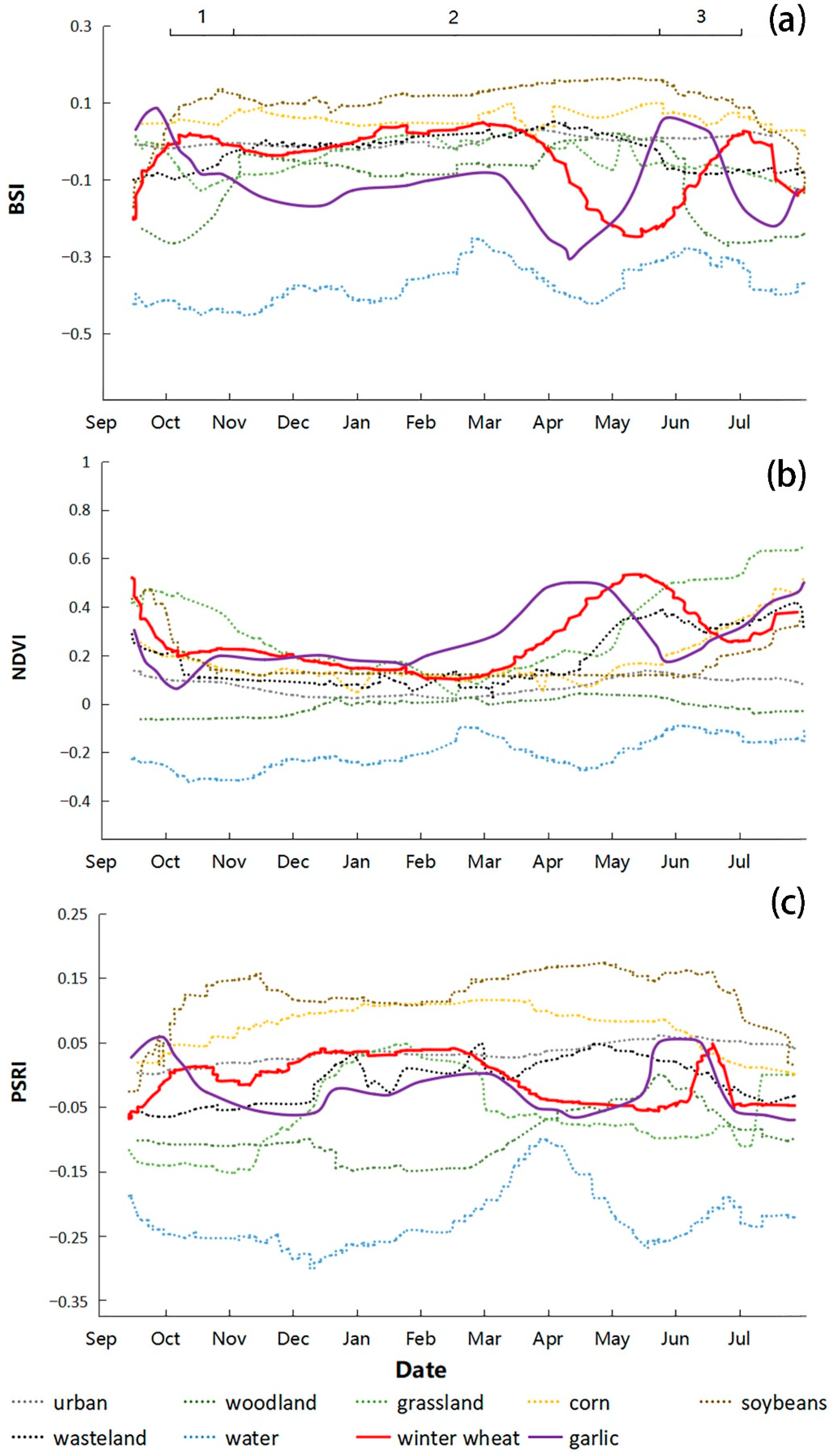
The study area in this work is the whole region of Beijing, the land cover types of it include urban area, woodland, grassland, an agricultural area, wasteland, and water. The urban area occupies the majority of the study area, its spectral profile is gentle without obvious phenological changes. The woodland in Beijing is mostly deciduous broadleaved [48], it begins to grow in spring and withers in winter, as does the grassland. Therefore, the lowest value of NDVI is in winter, it gradually rises in spring to summer, and reaches its peak in summer. The products planted in the Beijing agricultural area include winter wheat, corn, soybeans, and garlic [20,44]. Corn and soybeans are sown after the winter wheat harvest and harvested before the winter wheat sowing. In other words, the phenological characteristics of corn and soybean have complete distinctions from those of winter wheat. They do not grow in the growth cycle of winter wheat, so no matter the spectral profile of BSI, NDVI, or PSRI, they all tend to be stable. However, garlic is sown slightly later and harvested slightly earlier than winter wheat, which is always sown from late September to early October, wintered in December and January, and harvested from late May to early June of the following year [20,49]. Therefore, the phenological characteristic of garlic is similar to that of winter wheat, and it can be clearly seen from the spectral profiles that garlic reached the peak of BSI, NDVI, and PSRI earlier than winter wheat, which affected the classification accuracy of winter wheat to a certain extent. The spectral indices temporal profiles of different land cover types (pure pixels of each type selected from validation data, detailed selection of each validation data can be seen in Section 2.2.2), which were smoothed after SG filter in a full growth period of winter wheat, were drawn in Figure 5. The smoothing window of the SG filter used was 30 and the degree of smoothing polynomial was 3.
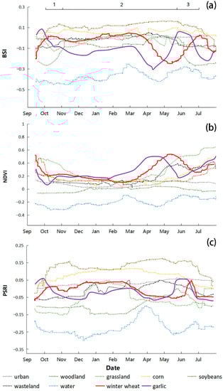
Figure 5.
Spectral indices temporal profiles of different land cover types in study area. Subfigure (a–c) are BSI, NDVI, and PSRI, respectively. The digits above the time series profiles denote key phenological periods of winter wheat. 1: sowing (1 October to 31), 2: growth (1 November to 19 May), 3: mature (20 May to 30 June).
Spectral separability is one of the key factors to determine the accuracy of winter wheat mapping. In this work, we used the Jeffries-Matusita (J-M) distance, which is a widely recognized measure of spectral separability [50], as an indicator to evaluate the spectral separability between winter wheat and other vegetation species. The formula is as below:
where represents the separability measure between winter wheat (represented as i) and garlic (represented as j), is the Bhattacharyya distance, and represent the means, and and represent the variance of two classes, respectively [51]. The range of JM distance is 0 to 2, a larger JM distance indicates a higher separability [52].
In order to display the performance of our classification method between the winter wheat and garlic, we conducted an experiment of classifying winter wheat and garlic classes. In the experiment, we compared the winter wheat map extracted using the Mpsf method mentioned above with the garlic map extracted using the same method. In the step of extracting garlic, we input garlic samples into OCSVM, and the parameter settings of the classifier are the same as those of winter wheat. The result can be seen in Section 3.1.
In order to verify the feasibility of the Mpsf method developed in this paper, we conducted comparative experiments on six spectral indices in three phenological periods. The composite images used in the experiment were constructed by using different spectral indices and phenological period combinations, and the combinations of each composite image are shown in Table 3. In addition, we randomly selected 50% from the validation data of winter wheat and garlic for evaluation. Garlic was selected from the ROI of non-winter wheat (mainly distributed in the suburbs of Shunyi, Miyun, and Huairou). Based on the above phenological analysis and existing studies [53], compared with other vegetation classes, garlic has the most similar spectral characteristics to winter wheat.
Table 3.
Phenological period combinations and their corresponding indices. Representation denotes the sequence number of different phenological periods.
2.3.3. One-Class Classifier
In addition to using the spectral indices temporal profiles of the multiple phenological periods of winter wheat to construct new features, the selection of a classifier is another important part of this mapping work. Since the only extraction species in this experiment was winter wheat, adopting a one-class classifier instead of a traditional multi-class classification method could improve the efficiency. OCSVM is a kind of support vector machine. By training normal data samples, an optimal hyperplane is established in the feature space, and the trained samples and their origin are separated according to the principle of maximizing the interval value [54]. As the training of OCSVM only needs one kind of sample, the time and manpower of collecting samples are greatly reduced. In the previous study [55], OCSVM was used to extract winter wheat with high accuracy. Therefore, the new feature of winter wheat (Mpsf) was put into OCSVM to obtain the mapping results in the Beijing area.
The Google Earth Engine uses LIBSVM for SVM classification [56], and it is an encapsulated function on the GEE platform. Since each GEE user can call it by inputting “ee.Classifier.libsvm” in the online code page to create an empty Support Vector Machine classifier, we can easily use the OCSVM function by setting the parameter “svmType” as “ONE_CLASS”, without the need for writing the algorithm code of OCSVM. In addition, choosing the appropriate kernel type and corresponding parameters is crucial for using an OCSVM classifier. According to the previous research [57], we used Radial Basis Function (RBF) as the kernel type of OCSVM in this work, and “gamma” and “nu” are 2 parameters that need to be set when using RBF as the kernel of OCSVM on the GEE platform. Since we put the composited winter wheat feature (one image) into OCSVM for training, other parameters (e.g., shrinking, degree, cost. Readers can query the specific meaning of each parameter from the GEE API Reference [58]) could be kept as default except for the values of “gamma” and “nu” which needed to be adjusted [9]. Each parameter we used for OCSVM in this method is shown in Table 4. When setting the “gamma” and “nu” parameters, we tried 0.1, 0.5, 1.0, 2.0, 2.5, and 5.0 for the “gamma” respectively, and 0.01, 0.1, 0.25, and 0.5 for the “nu”, respectively. We used the collected winter wheat samples to test the combination of each parameter and compared them with the reference data (see Section 2.2.2) to seek the highest precision parameter combinations. Finally, we found that in the experiments, for the winter wheat extraction in Beijing, the highest accuracy of “gamma” and “nu” were 5.0 and 0.1, respectively.
Table 4.
Parameters used for one-class classifier on Google Earth Engine platform in this paper.
2.4. Accuracy Assessment
In order to verify the accuracy of winter wheat mapping, we used three kinds of data to evaluate and consider the Mpsf mapping results: (1) Visual interpretation of winter wheat samples from Google Earth, (2) The official investigation of winter wheat provided by BBS, and (3) An open-source 30-m winter wheat-mapping product of the Beijing area for 2019 [59].
In comparison with the winter wheat sample data visually interpreted by Google Earth, we used four indicators to evaluate the accuracy of the Mpsf map (see Section 3.2.1): Producer Accuracy (PA), User Accuracy (UA), Overall Accuracy (OA), and kappa. Paper [60] introduced the construction of these four indicators in detail.
In comparison with the winter wheat data provided by BBS, we used two spatial dimension comparison methods: city-level and district-level. In the city-level method, we compared the winter wheat area of the whole of Beijing in an Mpsf map with statistical data from BBS and used the Relative Error (RE, Equation (3)) to measure the accuracy. In the comparison of the district-level, we used the coefficient of determination (R2) and root mean square error (RMSE, Equation (4)) to evaluate the winter wheat area correlation between the Mpsf map and BBS in 11 districts. It should be noted that there are a total of 16 districts in Beijing, but not every district planted winter wheat from 2018 to 2020 (reported from BBS), such as Dongcheng District, Xicheng District, and Fengtai District.
where and represent the data from Mpsf map and BBS, respectively.
where , , represent the mapping result, BBS data, and the number of districts (11) which planted winter wheat in the Beijing area, respectively.
Finally, in comparison with 30-m of mapping product, we firstly compared the whole winter wheat area in Beijing of this product and the Mpsf map with the data provided by BBS. Then, for the purpose of visual interpretation and specific classification results comparison of these two maps, we superimposed them on Sentinel-2 images, respectively.
3. Results
3.1. Spectral Separability
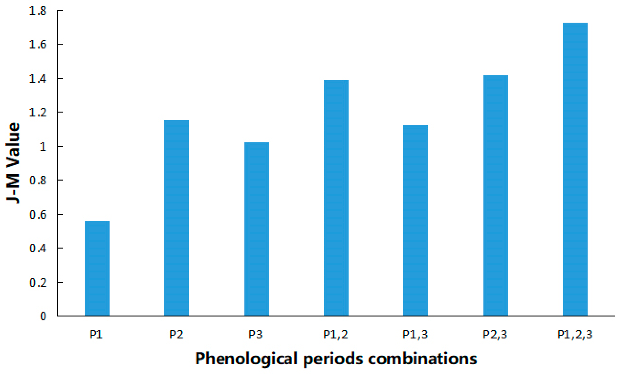
Figure 6 is a statistical histogram of spectral separability between winter wheat and garlic in seven phenological combinations of the study area. Among all of the combinations, the maximum value of J-M was reached (1.73) after using three phenological combinations, followed by two phenological combinations (ranging from 1.13 to 1.42) and, finally, the minimum value of J-M was obtained for a single phenological period (from 0.56 to 1.16). Overall, the J-M value of the Mpsf method, based on the composite of the three phenological periods and the corresponding six spectral indices, was the highest among the seven combinations. Therefore, winter wheat and garlic in the experiment, using the Mpsf method in this paper, had considerable spectral separability. In addition, we expect that the Mpsf method developed in our work may have a wide application for other types of crops in the future.

Figure 6.
J-M statistics of 7 phenological period combinations between winter wheat and garlic in Beijing. Details about the sequence number of different phenological periods is shown in Table 3.
It should be noted that the J-M value which used the phenological period of “growth” was higher than other combinations with the same number of phenological periods. For example, in a single phenological period spectral separability evaluation, P2 is higher than P1 and P3. When two phenological periods were used, the combination of P1,2 and P2,3 were higher than P1,3. Therefore, fully representing the phenological characteristics in a growth period is necessary to identify winter wheat in mapping work.
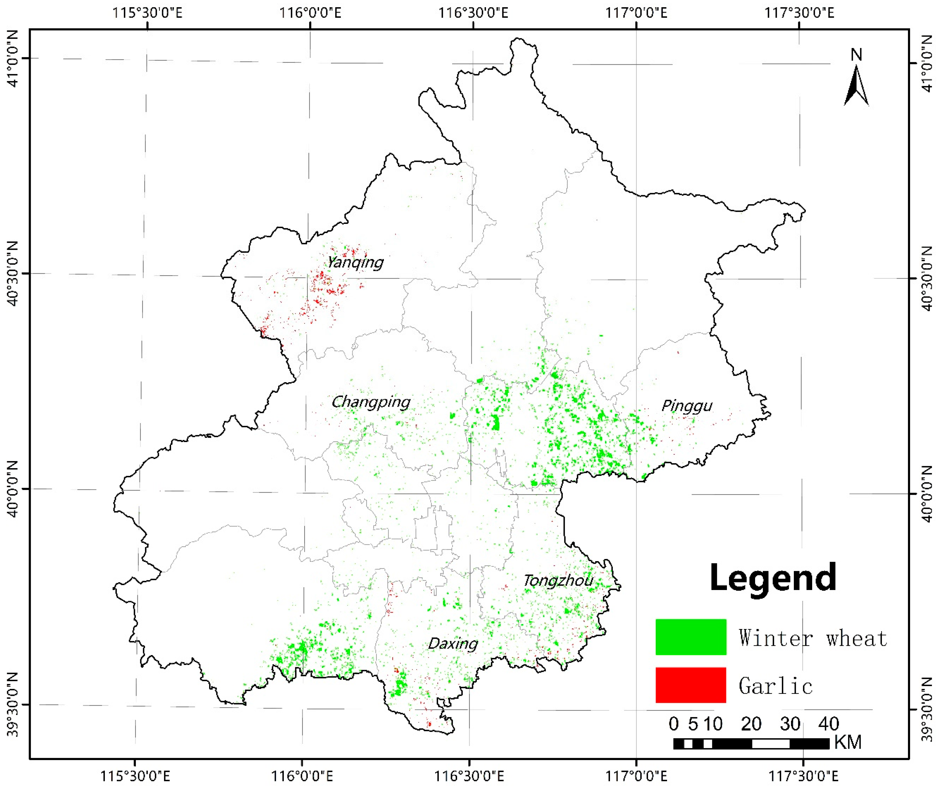
Figure 7 is the spatial winter wheat and garlic distribution of an Mpsf map in Beijing. From the extraction results, garlic was distributed and scattered in Yanqing, Pinggu, Daxing, Changping, and Tongzhou districts. We used the samples visually interpreted on the very high-resolution remote sensing images from Google Earth to evaluate the accuracy of garlic and winter wheat. The results are shown in Table 5.
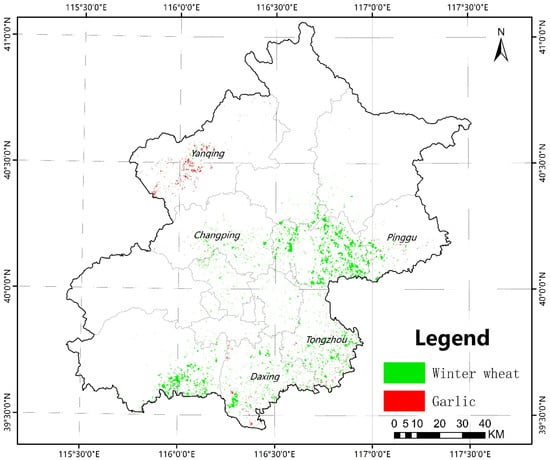
Figure 7.
Spatial winter wheat and garlic distribution of the Mpsf map in Beijing.
Table 5.
Confusion matrix of the winter wheat and garlic accuracy assessment (the 5 districts in which garlic was extracted).
As is shown in Table 5, the overall accuracy between winter wheat and garlic in five districts was not satisfactory. Although we showed the possibility of separating winter wheat and garlic with the J-M distance above, by using features in the entire phenological periods of winter wheat, the real classification of them turned out poor. However, it should be noted that in Beijing, the garlic cultivation area is small, and even too small to be considered a major agricultural product, according to the official website of BBS. Therefore, low classification accuracy between winter wheat and garlic will not harm the legitimacy of the entire study, in terms of the proposal of our study being to obtain the mapping product of winter wheat in the Beijing area by a rapid and operable method. Therefore, how to separate winter wheat from garlic accurately will be a challenging task in our future work.
3.2. Classification Accuracy
Based on the GEE cloud platform, we developed a new multiple phenological spectral feature for mapping winter wheat. Taking Beijing as the study area, Sentinel-2 data and the OCSVM classifier were used in this work for the refinement of winter wheat extraction. The mapping result is shown in Figure 8. In May, winter wheat is dark green in the remote sensing image. To fully demonstrate the Mpsf mapping, we superimposed the map results on false and true color composite images of the study area, respectively.
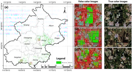
Figure 8.
Spatial winter wheat distribution of Mpsf map in Beijing. Sub-images on the right represent the identification of winter wheat in Fangshan District, Shunyi District, and Daxing District, respectively, and their specific position is indicated by red boxes in (a). The background images of (b–g) are Sentinel-2 data, which were taken on May 12, 2020. The three-band combination in (b–d): NIR, red, green. The three-band combination in (e–g): red, green, blue.
In order to verify the accuracy of the Mpsf map, we used three kinds of data to evaluate and consider the mapping results: (1) Visual interpretation of winter wheat samples from Google Earth. (2) The official investigation of winter wheat provided by BBS. (3) An open-source 30-m winter wheat-mapping product of the Beijing area in 2019.
3.2.1. Compare with Winter Wheat Sample Data
As shown in Table 6, the overall accuracy (OA) of the Mpsf map in the overall Beijing area was higher than 97.9%, and the kappa coefficient was 0.93. In the top three districts of the winter wheat planting area (Fangshan, shunyi, and Daxing), the winter wheat mapping method in this paper exhibited a good classification performance. The producer accuracy and user accuracy of the winter wheat category in the Fangshan district were 92.22% and 99.41% respectively. The producer accuracy and user accuracy in the Shunyi district were 96.98% and 99.68%, respectively. The producer accuracy and user accuracy in the Daxing district were 92.84% and 93.73%, respectively. Shunyi has the highest overall accuracy (OA: 99.05%), followed by Daxing (OA: 98.91%), and finally Fangshan (OA: 98.61%).
Table 6.
Confusion matrix of the winter wheat map accuracy assessment (the whole of Beijing and the 11 districts that planted winter wheat).
Although the overall accuracy of the Mpsf map was considerable in this work, there were still some limitations. Analysis of the uncertainty accuracy of mapping results can be seen in the discussion (Section 4.4).
3.2.2. Compare with Data from BBS
In comparison with the winter wheat data provided by BBS, we used two spatial dimension comparison methods: city-level and district-level. In the city-level method, we compared the winter wheat area of the whole of Beijing in the Mpsf map with statistical data from BBS and used RE to measure the accuracy. In the comparison of the district-level, we used the coefficient of determination (R2) and root mean square error (RMSE) to evaluate the winter wheat area correlation between the Mpsf map and BBS in 11 districts (Figure 9).
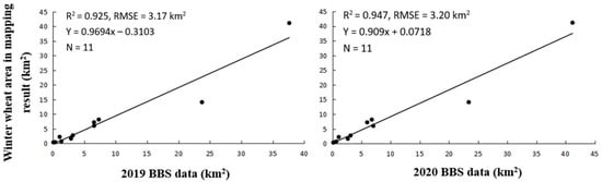
Figure 9.
District-level area comparison of winter wheat between the Mpsf map and data provided by BBS. The value of N represents the number of districts (11) which planted winter wheat in Beijing area (see Section 2.4 for details about the RMSE formula).
In the comparison of the district-level, the 2 years determination coefficient (R2) was 0.925 and 0.947, respectively. With the correlation (N = 11), RMSE was 3.17 km2 and 3.20 km2, respectively. Both results demonstrated that the Mpsf map was highly consistent with the statistical data (shown in Table 7).
Table 7.
Winter wheat area and relative error between mapping result and BBS.
3.2.3. Compare with a 30 m Winter Wheat-Mapping Product
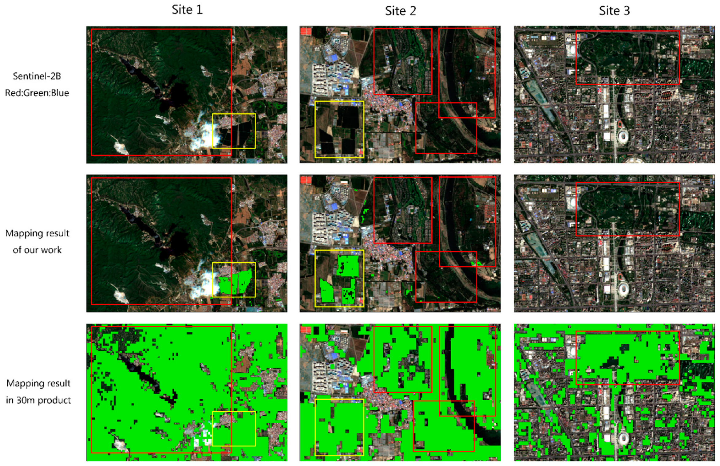
In comparison with a 30-m winter wheat-mapping product, we found that the product had many misclassifications between winter wheat and other surface features. We first compared the winter wheat area of the 30 m product and Mpsf map with the winter wheat data provided by BBS. Since this product only provided winter wheat data up to 2019, we could only use the data report of a single year from BBS (2019) for comparison. According to the statistical data, the area of winter wheat for Beijing in 2019 was 84.42 km2. The area obtained by the Mpsf method was 84.85 km2, while the area of the 30 m products was 1207.72 km2. In addition to the difference in the overall area, the classification of the 30 m product was relatively unsatisfactory. Figure 10 shows the situation of several sites between the Mpsf map and the 30 m product. The image used in the background is Sentinel-2B over Beijing on May 13, 2019, which was obtained in relative orbit 075, and the cloud cover percentage is 1.92%.
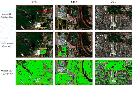
Figure 10.
Comparison between Mpsf map and 30 m product in Beijing. The different rows represent Sentinel-2 images (three-channel composite: red, green, blue), Mpsf map overlapping on Sentinel-2 images, and the 30 m product overlapping on Sentinel-2 images, respectively. The different columns represent different location sites. The yellow and red box regions show the ground truth winter wheat and misclassifications. Site 1: mountainous area. Site 2: rural area. Site 3: urban area.
Since the winter wheat mapping scale of this 30 m product was for the 11 provinces in China, it is understandable that the regional scale mapping accuracy in Beijing was not accurate. In our work, the misclassification of winter wheat has been alleviated. As shown in Figure 10, the comparison of the classification in the Mpsf map and 30 m product was listed. In the first column of Figure 10, the 30 m product classified many mountainous vegetations as winter wheat, while our product eliminated the confusion with the forest. In the second column of Figure 10, on account of the spectral features of other vegetation in the study area being similar to winter wheat, much other vegetation had been misclassified in the 30 m map, while our mapping result maintained a high classification accuracy. In the third column of Figure 10, there were artificial parks and grassland, which were excluded from our work, but the 30 m product classified them as winter wheat.
4. Discussion
4.1. Three Key Phenological Periods
Many previous studies have shown the feasibility of using phenological methods to extract winter wheat [61,62,63,64]. However, most of them used a single phenological period for winter wheat identification. Since there was no full description of the spectral features of the whole growth stages for winter wheat by methods, using a single phenological period to extract winter wheat may easily result in omission or misclassification.
In order to reduce the limitations mentioned above, we developed a Mpsf method, followed by using the generated new features as input data for OCSVM to map winter wheat.
During the sowing period, the vegetation coverage of fields planted with winter wheat was low, and soil information was highlighted. At this time, other vegetation around the winter wheat was in a flourishing state [20], such as woodland and grassland; they showed high values in NDVI temporal profile. So the BSI index was used to easily separate the winter wheat field from others. In the growth period, it took up the largest proportion in the whole growing stage of winter wheat, and the spectral features of winter wheat at this time were quite different from those of most surrounding vegetation. Especially in the spring regreening stage, woodland and grassland wintered during this time, and they showed low values of NDVI temporal profile. Other products planted in the agricultural area of Beijing (e.g., soybeans, corn) displayed stability in the whole growth cycle of winter wheat, in terms of their phenological periods, and were totally different from winter wheat. Therefore, it was one of the significant phenological periods [17] for extracting winter wheat. In the mature period, chlorophyll content of winter wheat decreased while carotenoids increased gradually. PSRI is a vegetation index which is sensitive to the changes in carotenoid and chlorophyll [34]. At the same time, woodland and grassland reached their peak values according to NDVI temporal profile. Thus, winter wheat can be well extracted from other vegetation classes by using the PSRI index [65,66] in its mature period.
4.2. Six Key Spectral Indices
In many previous studies, spectral indices were used to extract winter wheat, which had wide applicability [4,14,16,20]. For example, paper [67] used the NDVI index to extract winter wheat in Xinji City, Hebei Province and achieved good performance with an overall accuracy of 94.00%. Moreover, paper [49] used EVI index time series data to reconstruct the spatial-temporal change process of the winter wheat sown area in the North China Plain from 2001 to 2011. The indices used in the above studies were all for obtaining the spectral features of winter wheat in the growth stage, and they were not applicable to other stages. A single phenology cannot represent all spectral features of the whole growing stage of winter wheat. To remedy the limitation, six spectral indices were introduced to obtain spectral features of winter wheat at three different phenological stages.
The reason for selecting BSI in the sowing period was that BSI performed well in detecting the bare soil information [68]. For the growth period of winter wheat, we introduced GNDVI, NDVI6, and EVI to complement NDVI. With the change in environment, crop chlorophyll content also changes correspondingly, which had a good correlation with the value of SPAD (Soil and Plant Analyzer Development) [45,46]. The multispectral vegetation index with the highest correlation with SPAD value is GNDVI [39], which is why we chose GNDVI as a supplement. Moreover, paper [41] mentioned that NDVI is sensitive to the atmospheric environment, and paper [69] indicated that EVI was more accurate in detecting changes in canopy structure, so we introduced EVI to make up for the defects of NDVI. Finally, on account of NDVI being vulnerable to soil background noise [47], we introduced the NDVI6 index to overcome this limitation. Experiments in a previous study [40] showed that, compared with NDVI, NDVI6 had the better extraction performance for winter wheat. Due to the sensitivity of the PSRI index to carotenoids in senescent leaves [66], we selected it to determine the stages of maturity for winter wheat.
The median composite method has an excellent performance in reducing the influences of clouds, fog, and cloud shadows. Compared with other methods such as minimum, maximum, and mean composite methods, the median composite method can eliminate abnormally low or high values caused by clouds, fog, and cloud shadows in the same period. This is difficult to achieve by other methods. Moreover, the median composite method has been successfully applied in smoothing the spatial variability of crops. Experiments in the existing studies [70,71,72,73] have proved that the use of the median composite method can reduce the effects caused by different spectrums shared with the same plant species. However, it is worth noting that the median composite method still has shortcomings. For example, it cannot detect the peak of crop growth (e.g., winter wheat is at its peak NDVI value at the time of greening). Therefore, exploring a more robust composite method becomes the next step of our work.
From the results and accuracy of mapping in our work (see Section 3), the six spectral indices we selected were reasonable in extracting winter wheat. Each index showed different significant functions in multi-phenological stages of winter wheat. Therefore, we expect that through this Mpsf method, we can improve the shortcomings of traditional methods that cannot make full use of phenological features and need auxiliary data, and promote the development of winter wheat mapping at a regional scale. Therefore, in the future, we will keep up exploring the significance of other combinations of spectral indices with multiple phenological stages to improve the accuracy of winter wheat mapping.
4.3. One-Class Classifier
With the development of remote sensing technology in agriculture, the application of deep learning (DL) techniques in agricultural information detection is increasing. In the classification and monitoring of specific species, most applications still used multi-class classifiers; in these works, it was necessary to collect multiple types of samples and input them into the multi-class trainer, which is challenging and inefficient for classifying a class of interest [74]. In addition, the ratio between samples is not easy to set, which may lead to classification bias. Therefore, for remote sensing applications where the target species is only one class, using a one-class classifier is a better choice. Since these applications have only one class of training data, they can achieve good classification results in a short time by using the one-class classifier. In a previous study, OCSVM was used to extract winter wheat and high accuracy was obtained [75]. But in this study, the phenological information on winter wheat was not fully utilized. Therefore, we input the winter wheat features extracted from multiple phenological periods into OCSVM. From the accuracy of our mapping results, it is highly feasible and has a wide application prospect for the identification of other species. Although OCSVM performed well in the mapping of winter wheat, there is still room for improvement. First, in this experiment, we only tried the feasibility of OCSVM. Aside from OCSVM, one-class classifiers such as maximum entropy (MaxEnt), biased support vector machine (BSVM), and positive unlabeled learning (PUL), algorithms are also available [9]. In future work, we can continue to explore the impact of these other one-class classifiers on the accuracy of winter wheat mapping. Secondly, in recent years, DL methods have increasingly appeared in applications of remote sensing, which is one of the branches of machine learning. It was widely used in image target recognition and detection, and its accuracy and generalization ability were improved more than traditional methods [76]. However, there are still few studies combining DL methods with phenological knowledge for winter wheat mapping.
4.4. Implications and Uncertainty of the Winter Wheat Map
In this study, a 10 m resolution winter wheat-mapping product was produced for the Beijing area. As can be seen from the comparison of the Mpsf map with three reference data (see Section 2.2.2), this product has high accuracy. We believe that this is one of the most accurate winter wheat mapping results for the Beijing area to date, which is remarkable work. Therefore, we hope that this mapping work will contribute to the development of winter wheat mapping and provide a reference for sustainable agricultural development and governmental decision-making.
Although our winter wheat mapping result obtained a high accuracy, there are still some uncertainties. First of all, the reference winter wheat samples for this experiment were obtained from the historical images from GE; although GE provided very high-resolution historical images, there was a lack of images in some areas at specific time periods. Conducting surveys in the field can solve this limitation when conditions permit. Secondly, in some districts, the winter wheat classification accuracy was not satisfactory. As shown in Table 5, the producer accuracy of winter wheat in Haidian, Chaoyang, and Yanqing were 68.82%, 61.33%, and 66.67%, respectively, and the kappa of Chaoyang and Yanqing were 0.71 and 0.76, respectively. This was because the distribution of samples would affect the classification accuracy of OCSVM in a specific area. According to the principles of OCSVM, it constructed an optimal hyperplane in the feature space to maximize the margin between winter wheat and other classes. When we selected winter wheat samples for training, 75% of the winter wheat samples were from Fangshan, Shunyi, and Daxing, and the remaining 25% were from the rest of the eight districts. This proportion was set based on the data of winter wheat sown area from BBS, that is, the winter wheat sown area in Fangshan, Shunyi, and Daxing accounted for 75% of the total Beijing area. Therefore, fewer samples result in lower accuracy. But in terms of the classification accuracy of the whole of Beijing, our Mpsf method had satisfactory accuracy and could meet the needs of rapid and accurate winter wheat mapping. Thirdly, the location where winter wheat was planted is unlikely to remain the same for two years (mid-September 2018 to mid-July 2020). We compared the images of most of the sample areas during the key periods of winter wheat growth and tried to select the winter wheat fields which remain in the same location. However, due to the limitations of satellite revisit periods, we may not be able to check every ROI. Changes in the location of winter wheat planting areas within the study time interval reduced the accuracy of the final mapping results. Therefore, the use of other remote sensing data in combination with Sentinel-2 may solve this problem in future work. Thirdly, other crops or vegetation with the same phenological period as winter wheat in the study area may have affected the classification accuracy. Although the phenological features of winter wheat are different from almost crops and vegetation, there are exceptions. Garlic was the factor affecting the identification of winter wheat mostly in this study because its phenological period is similar to that of winter wheat: it is sown in late September to early October, overwintered in December and January, and ripened in late May to early June in the following year [20,49]. Therefore, the difference between the growth stages of garlic and winter wheat was slight. Although we have conducted spectral separability evaluation and proved that there was a significant spectral distinction between winter wheat and garlic using the Mpsf method, there have still been some misclassifications in winter wheat mapping. Therefore, the extraction of garlic from winter wheat will become the main task in future work. Several studies have explored the separation of winter wheat and garlic, which provide significant references for our future work. Due to the need for mulching after sowing, according to garlic cultivation, at the seedling stage, the vegetation index of garlic was lower than that of winter wheat, which is a characteristic point to distinguish between winter wheat and garlic [77]. Moreover, winter wheat showed up dark green, while garlic showed up bright green on the remote sensing images, because the blue, green, and red band reflectance of winter wheat are lower than garlic, and the reflectance value of the green band is higher than that of the blue and red band [49]. Therefore, we can use the mentioned methods to mask garlic to produce more accurate winter wheat-mapping products in the future. Finally, in this experiment, only the spectral features of pixels were used in the trainer. This method was simple and had strong feasibility, but it did not take into account the geospatial contextual information. Therefore, some noise points appeared in the mapping results. Thus, in future works, the combination of object-based image processing methods and Mpsf methods should be considered.
5. Conclusions
In this study, a new multiple phenological spectral feature for mapping winter wheat was developed, followed by the generation of new features as input data for a one-class of classifiers (OCSVM) to map winter wheat in the Beijing region. The Mpsf method maximized the spectral separability between winter wheat and other classes by combining three key phenological periods and calculating six spectral indices for the corresponding phenological periods to fully characterize the complete spectral characteristics of winter wheat in its lifespan. Since the data acquisition, processing, and analysis are implemented on the Google Earth Engine (GEE), this study has the potential to be migratory for monitoring and analysis. The cloud-based platform allows for rapid migration to other regions or other species, which has a higher potential for application than traditional local computing. In addition, we found good performance in extracting winter wheat using the Mpsf method. One of the most accurate winter wheat maps for 2019 and 2020 was obtained in this study at a spatial resolution of 10 m in the Beijing area, to date. We hope that this mapping work can contribute to the development of winter wheat mapping for sustainable agricultural development and governmental decision-making.
Author Contributions
Conceptualization, J.T.; methodology, W.C. and J.T.; software, W.C.; formal analysis, J.T. and W.C.; resources, J.T., X.L., L.Z. and B.C.; writing—original draft preparation, W.C.; writing—review and editing, W.C. and J.T. funding acquisition, X.L., L.Z. and B.C. All authors have read and agreed to the published version of the manuscript.
Funding
This research was funded by the National Natural Science Foundation of China (No. 42171330) and the Beijing Outstanding Young Scientist Program (No. BJJWZYJH01201910028032).
Data Availability Statement
Data sources were mentioned in the text, the code of the Mpsf method developed in our work, and the 10 m winter wheat-mapping product in Beijing area are available in a repository online. URL: https://github.com/EstherCai0330/A-new-multiple-phenological-spectral-feature-for-mapping-winter-wheat (accessed on 24 July 2022).
Acknowledgments
We sincerely thank the GEE team for providing free Sentinel-2 data and the computational platform. We also sincerely thank internal and external reviewers for their insights, which help improve the manuscript.
Conflicts of Interest
The authors declare no conflict of interest.
References
- Han, N.A.; Zhang, B.Z.; Liu, Y.; Peng, Z.G.; Zhou, Q.Y.; Wei, Z. Rapid Diagnosis of Nitrogen Nutrition Status in Summer Maize over Its Life Cycle by a Multi-Index Synergy Model Using Ground Hyperspectral and UAV Multispectral Sensor Data. Atmosphere 2022, 13, 122. [Google Scholar] [CrossRef]
- Fan, M.; Miao, F.; Jia, H.; Li, G.; Powers, C.; Nagarajan, R.; Alderman, P.D.; Carver, B.F.; Ma, Z.; Yan, L. O-linked N-acetylglucosamine transferase is involved in fine regulation of flowering time in winter wheat. Nat. Commun. 2021, 12, 2303. [Google Scholar] [CrossRef] [PubMed]
- Dong, Q.; Chen, X.; Chen, J.; Zhang, C.; Liu, L.; Cao, X.; Zang, Y.; Zhu, X.; Cui, X. Mapping Winter Wheat in North China Using Sentinel 2A/B Data: A Method Based on Phenology-Time Weighted Dynamic Time Warping. Remote Sens. 2020, 12, 1274. [Google Scholar] [CrossRef]
- Li, C.; Chen, W.; Wang, Y.; Wang, Y.; Ma, C.; Li, Y.; Li, J.; Zhai, W. Mapping Winter Wheat with Optical and SAR Images Based on Google Earth Engine in Henan Province, China. Remote Sens. 2022, 14, 284. [Google Scholar] [CrossRef]
- Useya, J.; Chen, S. Exploring the Potential of Mapping Cropping Patterns on Smallholder Scale Croplands Using Sentinel-1 SAR Data. Chin. Geogr. Sci. 2019, 29, 626–639. [Google Scholar] [CrossRef]
- Tiwari, V.; Matin, M.A.; Qamer, F.M.; Ellenburg, W.L.; Bajracharya, B.; Vadrevu, K.; Rushi, B.R.; Yusafi, W. Wheat Area Mapping in Afghanistan Based on Optical and SAR Time-Series Images in Google Earth Engine Cloud Environment. Front. Environ. Sci. 2020, 8, 77. [Google Scholar] [CrossRef]
- Mercier, A.; Betbeder, J.; Baudry, J.; Le Roux, V.; Spicher, F.; Lacoux, J.; Roger, D.; Hubert-Moy, L. Evaluation of Sentinel-1 & 2 time series for predicting wheat and rapeseed phenological stages. ISPRS J. Photogramm. Remote Sens. 2020, 163, 231–256. [Google Scholar] [CrossRef]
- Zhou, T.; Pan, J.; Zhang, P.; Wei, S.; Han, T. Mapping Winter Wheat with Multi-Temporal SAR and Optical Images in an Urban Agricultural Region. Sensors 2017, 17, 1210. [Google Scholar] [CrossRef]
- Ni, R.; Tian, J.; Li, X.; Yin, D.; Li, J.; Gong, H.; Zhang, J.; Zhu, L.; Wu, D. An enhanced pixel-based phenological feature for accurate paddy rice mapping with Sentinel-2 imagery in Google Earth Engine. ISPRS J. Photogramm. Remote Sens. 2021, 178, 282–296. [Google Scholar] [CrossRef]
- Liang, S.; Wang, J.; Jiang, B. Chapter 1—A systematic view of remote sensing. In Advanced Remote Sensing, 2nd ed.; Liang, S., Wang, J., Eds.; Academic Press: Cambridge, MA, USA, 2020; pp. 1–57. [Google Scholar]
- Liu, W.; Huang, J.; Wei, C.; Wang, X.; Mansaray, L.R.; Han, J.; Zhang, D.; Chen, Y. Mapping water-logging damage on winter wheat at parcel level using high spatial resolution satellite data. ISPRS J. Photogramm. Remote Sens. 2018, 142, 243–256. [Google Scholar] [CrossRef]
- Yuan, L.; Zhang, J.; Shi, Y.; Nie, C.; Wei, L.; Wang, J. Damage Mapping of Powdery Mildew in Winter Wheat with High-Resolution Satellite Image. Remote Sens. 2014, 6, 3611–3623. [Google Scholar] [CrossRef]
- Yang, Y.; Tao, B.; Ren, W.; Zourarakis, D.P.; El Masri, B.; Sun, Z.; Tian, Q. An Improved Approach Considering Intraclass Variability for Mapping Winter Wheat Using Multitemporal MODIS EVI Images. Remote Sens. 2019, 11, 1191. [Google Scholar] [CrossRef]
- Tao, J.-B.; Wu, W.-B.; Zhou, Y.; Wang, Y.; Jiang, Y. Mapping winter wheat using phenological feature of peak before winter on the North China Plain based on time-series MODIS data. J. Integr. Agric. 2017, 16, 348–359. [Google Scholar] [CrossRef]
- Ren, S.; Guo, B.; Wu, X.; Zhang, L.; Ji, M.; Wang, J. Winter wheat planted area monitoring and yield modeling using MODIS data in the Huang-Huai-Hai Plain, China. Comput. Electron. Agric. 2021, 182, 106049. [Google Scholar] [CrossRef]
- Li, F.; Ren, J.; Wu, S.; Zhao, H.; Zhang, N. Comparison of Regional Winter Wheat Mapping Results from Different Similarity Measurement Indicators of NDVI Time Series and Their Optimized Thresholds. Remote Sens. 2021, 13, 1162. [Google Scholar] [CrossRef]
- Dong, J.; Fu, Y.; Wang, J.; Tian, H.; Fu, S.; Niu, Z.; Han, W.; Zheng, Y.; Huang, J.; Yuan, W. Early-season mapping of winter wheat in China based on Landsat and Sentinel images. Earth Syst. Sci. Data 2020, 12, 3081–3095. [Google Scholar] [CrossRef]
- Meng, S.; Zhong, Y.; Luo, C.; Hu, X.; Wang, X.; Huang, S. Optimal Temporal Window Selection for Winter Wheat and Rapeseed Mapping with Sentinel-2 Images: A Case Study of Zhongxiang in China. Remote Sens. 2020, 12, 226. [Google Scholar] [CrossRef]
- Hunt, M.L.; Blackburn, G.A.; Carrasco, L.; Redhead, J.W.; Rowland, C.S. High resolution wheat yield mapping using Sentinel-2. Remote Sens. Environ. 2019, 233, 111410. [Google Scholar] [CrossRef]
- Qu, C.; Li, P.; Zhang, C. A spectral index for winter wheat mapping using multi-temporal Landsat NDVI data of key growth stages. ISPRS J. Photogramm. Remote Sens. 2021, 175, 431–447. [Google Scholar] [CrossRef]
- Wang, C.; Zhang, H.; Wu, X.; Yang, W.; Shen, Y.; Lu, B.; Wang, J. AUTS: A Novel Approach to Mapping Winter Wheat by Automatically Updating Training Samples Based on NDVI Time Series. Agriculture 2022, 12, 817. [Google Scholar] [CrossRef]
- Pan, L.; Xia, H.; Zhao, X.; Guo, Y.; Qin, Y. Mapping Winter Crops Using a Phenology Algorithm, Time-Series Sentinel-2 and Landsat-7/8 Images, and Google Earth Engine. Remote Sens. 2021, 13, 2510. [Google Scholar] [CrossRef]
- Liu, L.; Cao, R.; Chen, J.; Shen, M.; Wang, S.; Zhou, J.; He, B. Detecting crop phenology from vegetation index time-series data by improved shape model fitting in each phenological stage. Remote Sens. Environ. 2022, 277, 113060. [Google Scholar] [CrossRef]
- Jiang, L.; Shang, S.; Yang, Y.; Guan, H. Mapping interannual variability of maize cover in a large irrigation district using a vegetation index—Phenological index classifier. Comput. Electron. Agric. 2016, 123, 351–361. [Google Scholar] [CrossRef]
- Zhang, X.; Xiao, X.; Wang, X.; Xu, X.; Chen, B.; Wang, J.; Ma, J.; Zhao, B.; Li, B. Quantifying expansion and removal of Spartina alterniflora on Chongming island, China, using time series Landsat images during 1995–2018. Remote Sens. Environ. 2020, 247, 111916. [Google Scholar] [CrossRef] [PubMed]
- Kennedy, R.E.; Yang, Z.; Cohen, W.B. Detecting trends in forest disturbance and recovery using yearly Landsat time series: 1. LandTrendr—Temporal segmentation algorithms. Remote Sens. Environ. 2010, 114, 2897–2910. [Google Scholar] [CrossRef]
- Huang, C.; Goward, S.N.; Masek, J.G.; Thomas, N.; Zhu, Z.; Vogelmann, J.E. An automated approach for reconstructing recent forest disturbance history using dense Landsat time series stacks. Remote Sens. Environ. 2010, 114, 183–198. [Google Scholar] [CrossRef]
- Hermosilla, T.; Wulder, M.; White, J.; Coops, N.C.; Hobart, G.W.; Campbell, L.B. Mass data processing of time series Landsat imagery: Pixels to data products for forest monitoring. Int. J. Digit. Earth 2016, 9, 1035–1054. [Google Scholar] [CrossRef]
- Tian, J.; Wang, L.; Yin, D.; Li, X.; Diao, C.; Gong, H.; Shi, C.; Menenti, M.; Ge, Y.; Nie, S.; et al. Development of spectral-phenological features for deep learning to understand Spartina alterniflora invasion. Remote Sens. Environ. 2020, 242, 111745. [Google Scholar] [CrossRef]
- Weigand, M.; Staab, J.; Wurm, M.; Taubenböck, H. Spatial and semantic effects of LUCAS samples on fully automated land use/land cover classification in high-resolution Sentinel-2 data. Int. J. Appl. Earth Obs. Geoinf. 2020, 88, 102065. [Google Scholar] [CrossRef]
- Polykretis, C.; Grillakis, M.; Alexakis, D. Exploring the Impact of Various Spectral Indices on Land Cover Change Detection Using Change Vector Analysis: A Case Study of Crete Island, Greece. Remote Sens. 2020, 12, 319. [Google Scholar] [CrossRef] [Green Version]
- Chu, H.; Venevsky, S.; Wu, C.; Wang, M. NDVI-based vegetation dynamics and its response to climate changes at Amur-Heilongjiang River Basin from 1982 to 2015. Sci. Total Environ. 2018, 650, 2051–2062. [Google Scholar] [CrossRef]
- De Castro, A.I.; Six, J.; Plant, R.E.; Peña, J.M. Mapping Crop Calendar Events and Phenology-Related Metrics at the Parcel Level by Object-Based Image Analysis (OBIA) of MODIS-NDVI Time-Series: A Case Study in Central California. Remote Sens. 2018, 10, 1745. [Google Scholar] [CrossRef]
- Merzlyak, M.N.; Gitelson, A.A.; Chivkunova, O.B.; Rakitin, V.Y. Non-destructive optical detection of pigment changes during leaf senescence and fruit ripening. Physiol. Plant. 1999, 106, 135–141. [Google Scholar] [CrossRef]
- Ren, S.; Chen, X.; An, S. Assessing plant senescence reflectance index-retrieved vegetation phenology and its spatiotemporal response to climate change in the Inner Mongolian Grassland. Int. J. Biometeorol. 2016, 61, 601–612. [Google Scholar] [CrossRef]
- Chen, J.; Jönsson, P.; Tamura, M.; Gu, Z.; Matsushita, B.; Eklundh, L. A simple method for reconstructing a high-quality NDVI time-series data set based on the Savitzky–Golay filter. Remote Sens. Environ. 2004, 91, 332–344. [Google Scholar] [CrossRef]
- Bera, B.; Saha, S.; Bhattacharjee, S. Forest cover dynamics (1998 to 2019) and prediction of deforestation probability using binary logistic regression (BLR) model of Silabati watershed, India. Trees For. People 2020, 2, 100034. [Google Scholar] [CrossRef]
- Tucker, C.J. Red and photographic infrared linear combinations for monitoring vegetation. Remote Sens. Environ. 1979, 8, 127–150. [Google Scholar] [CrossRef]
- Niu, Q.L.; Feng, H.K.; Zhou, X.G.; Zhu, J.Q.; Yong, B.B.; Li, H.Z. Combining UAV Visible Light and Multispectral Vegetation Indices for Estimating SPAD Value of Winter Wheat. Trans. Chin. Soc. Agric. Mach. 2021, 52, 183–194. [Google Scholar]
- Chen, S.X.; Xu, X.G.; Xu, L.J.; Yang, G.J.; Xing, H.M.; He, P. Estimating Vegetation Coverage of Winter Wheat Based on New Vegetation Index. J. Triticeae Crops 2016, 36, 939–944. [Google Scholar]
- Huete, A.; Didan, K.; Miura, T.; Rodriguez, E.P.; Gao, X.; Ferreira, L.G. Overview of the radiometric and biophysical performance of the MODIS vegetation indices. Remote Sens. Environ. 2002, 83, 195–213. [Google Scholar] [CrossRef]
- Huete, A.R.; Liu, H.Q.; Batchily, K.V.; van Leeuwen, W. A comparison of vegetation indices over a global set of TM images for EOS-MODIS. Remote Sens. Environ. 1997, 59, 440–451. [Google Scholar] [CrossRef]
- Khan, A.; Hansen, M.C.; Potapov, P.V.; Adusei, B.; Pickens, A.; Krylov, A.; Stehman, S.V. Evaluating Landsat and RapidEye Data for Winter Wheat Mapping and Area Estimation in Punjab, Pakistan. Remote Sens. 2018, 10, 489. [Google Scholar] [CrossRef] [Green Version]
- Tian, H.; Pei, J.; Huang, J.; Li, X.; Wang, J.; Zhou, B.; Qin, Y.; Wang, L. Garlic and Winter Wheat Identification Based on Active and Passive Satellite Imagery and the Google Earth Engine in Northern China. Remote Sens. 2020, 12, 3539. [Google Scholar] [CrossRef]
- Darvishzadeh, R.; Skidmore, A.; Schlerf, M.; Atzberger, C.; Corsi, F.; Cho, M. LAI and chlorophyll estimation for a heterogeneous grassland using hyperspectral measurements. ISPRS J. Photogramm. Remote Sens. 2008, 63, 409–426. [Google Scholar] [CrossRef]
- Kawashima, S.; Nakatani, M. An Algorithm for Estimating Chlorophyll Content in Leaves Using a Video Camera. Ann. Bot. 1998, 81, 49–54. [Google Scholar] [CrossRef]
- Wang, Z.X.; Liu, C.; Alfredo, H. From AVHRR-NDVI to MODIS-EVI: Advances in vegetation index research. Acta Ecol. Sin. 2003, 23, 979–987. [Google Scholar]
- Chen, Y.Y. The Main Tree Species in Typital Areas of Beijing Regulate the Air Quality and Ecological Function. Master’s Thesis, University of Agriculture, Beijing, China, 2019. [Google Scholar]
- Li, F.; Xie, L.; Wang, H.; Qin, Q.; Zhao, H. Extraction and annual variation dynamic monitoring of winter wheat area based on GF-1 images. Shandong Agric. Sci. 2017, 49, 139–144. [Google Scholar] [CrossRef]
- Tolpekin, V.A.; Stein, A. Quantification of the Effects of Land-Cover-Class Spectral Separability on the Accuracy of Markov-Random-Field-Based Superresolution Mapping. IEEE Trans. Geosci. Remote Sens. 2009, 47, 3283–3297. [Google Scholar] [CrossRef]
- Wang, Y.; Qi, Q.; Liu, Y. Unsupervised Segmentation Evaluation Using Area-Weighted Variance and Jeffries-Matusita Distance for Remote Sensing Images. Remote Sens. 2018, 10, 1193. [Google Scholar] [CrossRef]
- Schmidt, K.; Skidmore, A. Spectral discrimination of vegetation types in a coastal wetland. Remote Sens. Environ. 2003, 85, 92–108. [Google Scholar] [CrossRef]
- Zhang, H.; Du, H.; Zhang, C.; Zhang, L. An automated early-season method to map winter wheat using time-series Sentinel-2 data: A case study of Shandong, China. Comput. Electron. Agric. 2021, 182, 105962. [Google Scholar] [CrossRef]
- Schölkopf, B.; Platt, J.C.; Shawe-Taylor, J.; Smola, A.J.; Williamson, R.C. Estimating the Support of a High-Dimensional Distribution. Neural Comput. 2001, 13, 1443–1471. [Google Scholar] [CrossRef] [PubMed]
- Yang, G.; Yu, W.; Yao, X.; Zheng, H.; Cao, Q.; Zhu, Y.; Cao, W.; Cheng, T. AGTOC: A novel approach to winter wheat mapping by automatic generation of training samples and one-class classification on Google Earth Engine. Int. J. Appl. Earth Obs. Geoinform. 2021, 102, 102446. [Google Scholar] [CrossRef]
- Chang, C.; Lin, C. LIBSVM: A Library for Support Vector Machines. ACM Trans. Intell. Syst. Technol. 2011, 2, 1–27. [Google Scholar] [CrossRef]
- Xiao, Y.; Wang, H.; Xu, W. Parameter Selection of Gaussian Kernel for One-Class SVM. IEEE Trans. Cybern. 2014, 45, 941–953. [Google Scholar] [CrossRef]
- Gorelick, N.; Hancher, M.; Dixon, M.; Ilyushchenko, S.; Thau, D.; Moore, R. Google Earth Engine: Planetary-scale geospatial analysis for everyone. Remote Sens. Environ. 2017, 202, 18–27. [Google Scholar] [CrossRef]
- Dong, J.; Fu, Y.; Wang, J.; Tian, H.; Fu, S.; Niu, Z.; Han, W.; Zheng, Y.; Huang, J.; Yaun, W. 30 m Winter Wheat Distribution Map of China for Four Years (2016–2019). figshare 2020. [Google Scholar] [CrossRef]
- Foody, G.M. Impacts of ignorance on the accuracy of image classification and thematic mapping. Remote Sens. Environ. 2021, 259, 112367. [Google Scholar] [CrossRef]
- Lu, L.L.; Wang, C.Z.; Guo, H.D.; Li, Q.T. Detecting winter wheat phenology with SPOT-VEGETATION data in the North China Plain. Geocarto Int. 2014, 29, 244–255. [Google Scholar] [CrossRef]
- Tian, J.; Zhu, X.; Shen, Z.; Wu, J.; Xu, S.; Liang, Z.; Wang, J. Investigating the urban-induced microclimate effects on winter wheat spring phenology using Sentinel-2 time series. Agric. For. Meteorol. 2020, 294, 108153. [Google Scholar] [CrossRef]
- Song, Y.; Wang, J. Mapping Winter Wheat Planting Area and Monitoring Its Phenology Using Sentinel-1 Backscatter Time Series. Remote Sens. 2019, 11, 449. [Google Scholar] [CrossRef]
- Qiu, B.; Luo, Y.; Tang, Z.; Chen, C.; Lu, D.; Huang, H.; Chen, Y.; Chen, N.; Xu, W. Winter wheat mapping combining variations before and after estimated heading dates. ISPRS J. Photogramm. Remote Sens. 2017, 123, 35–46. [Google Scholar] [CrossRef]
- Cai, Y.; Lin, H.; Zhang, M. Mapping paddy rice by the object-based random forest method using time series Sentinel-1/Sentinel-2 data. Adv. Space Res. 2019, 64, 2233–2244. [Google Scholar] [CrossRef]
- Anderegg, J.; Yu, K.; Aasen, H.; Walter, A.; Liebisch, F.; Hund, A. Spectral Vegetation Indices to Track Senescence Dynamics in Diverse Wheat Germplasm. Front. Plant Sci. 2020, 10, 1749. [Google Scholar] [CrossRef] [PubMed]
- Wang, D.L.; Zhang, A.B.; Zhao, A.Z.; Li, J. Extraction model of winter wheat planting information based on unsupervised classification. Bull. Surv. Mapp. 2019, 8, 68–71+77. [Google Scholar] [CrossRef]
- Bera, B.; Saha, S.; Bhattacharjee, S. Estimation of Forest Canopy Cover and Forest Fragmentation Mapping Using Landsat Satellite Data of Silabati River Basin (India). KN-J. Cartogr. Geogr. Inf. 2020, 70, 181–197. [Google Scholar] [CrossRef]
- Pastor-Guzman, J.; Dash, J.; Atkinson, P.M. Remote sensing of mangrove forest phenology and its environmental drivers. Remote Sens. Environ. 2018, 205, 71–84. [Google Scholar] [CrossRef]
- Azzari, G.; Lobell, D. Landsat-based classification in the cloud: An opportunity for a paradigm shift in land cover monitoring. Remote Sens. Environ. 2017, 202, 64–74. [Google Scholar] [CrossRef]
- Bey, A.; Jetimane, J.; Lisboa, S.N.; Ribeiro, N.; Sitoe, A.; Meyfroidt, P. Mapping smallholder and large-scale cropland dynamics with a flexible classification system and pixel-based composites in an emerging frontier of Mozambique. Remote Sens. Environ. 2020, 239, 111611. [Google Scholar] [CrossRef]
- Flood, N. Seasonal Composite Landsat TM/ETM+ Images Using the Medoid (a Multi-Dimensional Median). Remote Sens. 2013, 5, 6481–6500. [Google Scholar] [CrossRef]
- Jin, Z.; Azzari, G.; You, C.; Di Tommaso, S.; Aston, S.; Burke, M.; Lobell, D.B. Smallholder maize area and yield mapping at national scales with Google Earth Engine. Remote Sens. Environ. 2019, 228, 115–128. [Google Scholar] [CrossRef]
- Mack, B.; Roscher, R.; Stenzel, S.; Feilhauer, H.; Schmidtlein, S.; Waske, B. Mapping raised bogs with an iterative one-class classification approach. ISPRS J. Photogramm. Remote Sens. 2016, 120, 53–64. [Google Scholar] [CrossRef]
- Zhao, L.; Li, Q.; Zhang, Y.; Du, X.; Wang, H.; Shen, Y. Study on the potential of whitening transformation in improving single crop mapping accuracy. J. Appl. Remote Sens. 2019, 13, 034512. [Google Scholar] [CrossRef]
- Sun, H.; Li, S.; Li, M.Z.; Liu, H.J.; Qiao, L.; Zhang, Y. Research Progress of Image Sensing and Deep Learning in Agriculture. Trans. Chin. Soc. Agric. Mach. 2020, 51, 1–17. [Google Scholar]
- Cai, W. Wheat Identification and Area Estimation Based on Mixed Image Element Decomposition of MODIS Remote Sensing Data. Master’s Thesis, Shandong Normal University, Jinan, China, 2010. [Google Scholar]


Publisher’s Note: MDPI stays neutral with regard to jurisdictional claims in published maps and institutional affiliations. |
© 2022 by the authors. Licensee MDPI, Basel, Switzerland. This article is an open access article distributed under the terms and conditions of the Creative Commons Attribution (CC BY) license (https://creativecommons.org/licenses/by/4.0/).