Article

Modelling and Assessment of a New Triple-Frequency IF1213 PPP with BDS/GPS

1
School of Environmental and Spatial Informatics, China University of Mining and Technology, Xuzhou 221116, China
2
Qianxun Spatial Intelligence Inc., Shanghai 200082, China
3
School of Spatial Information and Geomatics Engineering, Anhui University of Science and Technology, Huainan 232001, China
*
Author to whom correspondence should be addressed.
Remote Sens. 2022, 14(18), 4509; https://doi.org/10.3390/rs14184509
Submission received: 19 July 2022 / Revised: 6 September 2022 / Accepted: 7 September 2022 / Published: 9 September 2022
(This article belongs to the Special Issue BDS/GNSS for Earth Observation)

Abstract

:
The currently available triple-frequency signals give rise to new prospects for precise point positioning (PPP). However, they also bring new bias, such as time-varying parts of the phase bias in the hardware of receivers and satellites due to the fact that dual-frequency precise clock products cannot be directly applied to triple-frequency observation. These parameters generate phase-based inter-frequency clock bias (PIFCB), which impacts the PPP. However, the PIFCBs of satellites are not present in all GNSSs. In this paper, various IF1213 PPP models are constructed for these parts, namely, the triple-frequency PIFCB (TF-C) model with PIFCB estimation, the TF inter-frequency bias (IFB) (TF-F) model ignoring the PIFCB, and the TF-PIFCB-IFB (TF-CF) model with one system PIFCB estimation. Additionally, this study compares these IF1213 PPP models with the dual-frequency ionosphere-free (DF) model. We conducted single system static PPP, dual-system static and kinematic PPP experiments based on BDS/GPS observation data. The GPS static PPP experiment demonstrates the reliability of the TF-C model, as well as the non-negligibility of the GPS PIFCB. The BDS static PPP experiment demonstrates the reliability of the TF-F and TF-CF models, and that the influence of the BDS-2 PIFCB can be neglected in BDS. The BDS/GPS PPP experimental results show that the third frequency does not significantly improve the positioning accuracy but shortens the convergence time. The positioning accuracy of TF-C and TF-CF for static PPP is better than 1.0 cm, while that for kinematic PPP is better than 2.0 cm and 4.0 cm in the horizontal and vertical components, respectively. Compared with the DF model, the convergence time of the TF-C and TF-CF models for static PPP is improved by approximately 23.5%/18.1%, 13.6%/9.7%, and 19.8%/12.1%, while that for kinematic PPP is improved by approximately 46.2%/49.6%, 33.5%/32.4%, and 35.1%/36.1% in the E, N and U directions, respectively. For dual-system PPP based on BDS/GPS observations, the TF-C model is recommended.

Graphical Abstract

1. Introduction

In the late 1990s, precise point positioning (PPP) technology was proposed by Zumberge et al. [1] and implemented [2]. With the modernization of GPS and the completion of BDS, an increasing number of navigation satellites provide signals at three or more frequencies, and the research and application of triple-frequency PPP has become increasingly extensive and in depth [3,4,5,6]. The available triple-frequency signals create new prospects for integrity monitoring [7], for facilitating cycle slip detection and repairing [8,9], for fast ambiguity resolution (AR) [10] and for ionospheric analysis [11]. While triple-frequency signals have many benefits, new bias has also been introduced. Montenbruck et al. [12] first demonstrated the existence of a bias between L1/L2 and L1/L5 in ionosphere-free (IF) combination, including a periodic line bias between the satellite and the signal, based on geometry-free and ionosphere-free (GFIF) phase combination. The inconsistency of L1/L2/L5 was defined as inter-frequency clock bias (IFCB) [13]. Precise clock estimation (PCE) is obtained through dual-frequency IF combination. When using signals of different frequencies for the dual-frequency IF combination PCE, the satellite clock estimation will have a bias, which is the IFCB [14]. The bias consists of the receiver and satellite code hardware bias and phase hardware bias time-varying components, which generate the code-based IFCB (CIFCB) and PIFCB, respectively. The PIFCB consists of a satellite PIFCB and a receiver PIFCB. However, not all satellites of constellations have PIFCB, e.g., BDS-3, Galileo and QZSS constellations could ignore the satellite PIFCB [15,16].
GPS Block IIF satellite PIFCB varies throughout the day, with peak-to-peak amplitudes of a few to several tens of centimeters [13]. Pan et al. [14] proposed a satellite PIFCB estimation method for triple-frequency PPP for GPS and established an uncombined (UC) and IF123 PPP model with satellite PIFCB estimations followed by corrections. The experimental results showed that after GPS satellite PIFCB corrections, the corresponding positioning accuracy of the UC123 and IF123 PPP models could be improved to 5, 4, and 9 mm and 4, 3, and 10 mm in the E, N and U directions, respectively. For BDS-2, there was a small bias in B1I/B2I/B3I, and its satellite PIFCB varied throughout the day with a peak-to-peak amplitude of approximately 2 cm [17,18]. Fan et al. [19] proposed a GNSS IFCB estimation and correction generic model, which was implemented and validated using BDS-2 and BDS-3 data. It was experimentally demonstrated that the BDS-2 satellite PIFCB showed a periodic variation and with some of the satellites corrected by PIFCB, the mean root mean square error (RMS) value of the GFIF phase combination was 5 mm, which was an improvement of 50%. Gong et al. [20] and Pan et al. [21] systematically studied the long-term characteristics of the GNSS satellite PIFCB through GFIF phase combination.
In addition to the study of the characteristics of the satellite PIFCB, a number of researchers have analyzed different triple-frequency PPP models based on the consideration of the satellite PIFCB [3,22]. Guo et al. [23] conducted a systematic study of the UC123, IF1213 and IF123 PPP models based on BDS-2 B1I/B2I/B3I triple-frequency observation data. Pan et al. [24] systematically analyzed different triple-frequency PPP models based on GPS triple-frequency observation data. Different studies have shown that triple-frequency PPP positioning performance considering satellite PIFCB could reach the level of dual-frequency PPP. As GPS, GLONASS, BDS and Galileo continue to improve and modernize, an increasing number of researchers are focusing on multi-constellation combinations [25,26,27,28], while multi-constellation multifrequency PPP is also a new trend. Li et al. [29] investigated the performance of BDS/Galileo for triple-frequency PPP AR, and Li et al. [10] investigated the performance of GPS/Galileo/BDS-2 for triple-frequency PPP AR. Different studies have shown that multi-GNSS positioning performance is not only better than single GNSS, but further improves position estimation and can be applied to complex environmental conditions.
In summary, the short- and long-term characteristics of the satellite PIFCB have been studied, as well as the triple-frequency PPP in the case of satellite PIFCB correction. In this study, we focus on the precision modeling of the dual-system triple-frequency IF1213 PPP and validate it using GPS and BDS observations. First, the IF1213 PPP models with different treatments for the PIFCB are presented, namely, triple-frequency PIFCB (TF-C) with the PIFCB estimation, triple-frequency IFB (TF-F) ignoring the PIFCB, and the triple-frequency PIFCB-IFB (TF-CF) model without the full estimation of PIFCB, which only estimates the PIFCB in one system. Additionally, we also present the IF1213 PPP model using the IGMAS [30] product corrected by the satellite PIFCB, namely, the triple-frequency IFB-product (TF-FP). The relationships between these models are also analyzed. Next, the deduced models are validated using BDS and GPS triple-frequency observations, respectively. GPS triple-frequency observations are also used to validate the influence of GPS PIFCB. BDS triple-frequency observations are also used to validate the influence of BDS-2 PIFCB in BDS. Static and kinematic experiments are then conducted using BDS/GPS triple-frequency data. Finally, the main conclusions are given.

2. Materials and Methods

In this section, the functional models of three IF1213 models (TF-C, TF-F, and TF-CF) are described based on the general observation model. Additionally, the TF–FP model is also presented. For convenience, the three frequencies are numbered 1, 2 and 3. The specific frequencies indicated by the numbers are shown in Table 1, and the values in parentheses are in MHz. For BDS-3, the IF combination of B1I/B1C causes the noise amplification factor to be much larger than that of B3I/B1C. Therefore, the IF13 combination utilizes the IF combination of B3I/B1C; this means that for BDS-3, the IF combination is IF1223 in the experiment, but it is still noted as IF1213 during the derivation of the model below for ease of expression.

2.1. General Observation Model

The code and carrier phase observations on a single frequency are as follows [31]:
{ p r , j s , Q = μ r s , Q x + d t r d t s , Q + m s , Q Z r + γ j I r , 1 s , Q + d r , j d j s , Q + ε r , j s , Q l r , j s , Q = μ r s , Q x + d t r d t s , Q + m s , Q Z r γ j I r , 1 s , Q + N r , j s , Q + φ r , j φ j s , Q + ξ r , j s , Q
where the superscript s , Q and subscript r represent the satellite, constellation and receiver, respectively; in this paper Q can be G, C2, C3 and C for GPS, BDS-2, BDS-3 and BDS, respectively, where BDS means that BDS-2 and BDS-3 are considered as one constellation; p r , j s , Q and l r , j s , Q are the code and phase observed-minus-computed (OMC) values, respectively; j denotes the frequency ( j = 1 , 2 , 3 ); μ r s , Q is the unit vector of direction; x represents the vector of position correction to the a priori position; and d t r and d t s , Q indicate the receiver and satellite clock offsets, respectively. Furthermore, Z r is the wet troposphere delay at zenith; γ j = f 1 2 / f j 2 is the ionospheric factor; f indicates the carrier phase frequency; I r , 1 s , Q denotes the slant ionospheric delay at the first frequency; and N r , j s , Q represents the integer phase ambiguity. The parameters d r , j and d j s , Q are the code hardware delays from the receiver and satellite, respectively. φ r , j and φ j s , Q are the receiver-dependent and satellite-dependent carrier phase hardware delays, respectively. ε r , j s , Q and ξ r , j s , Q are the measurement noise of the code and carrier phase, respectively. Other error items include the phase center offset (PCO) and variation (PCV), dry slant troposphere delay, phase wind-up, and relativistic effect. For simplicity, they are precisely corrected with their corresponding models and are not listed in the equations. It should be noted that in the case of lacking the precise PCO/PCV information of the third frequency, we use the PCO/PCV corrections of the first frequency instead due to the adjacent frequency.
For code and phase hardware bias, the code hardware bias is generally considered to be relatively stable and can be considered constant over the course of a day [32]. The phase hardware bias has a clear time-varying character and can be decomposed into a constant part and a time-varying part [13,14].
{ φ r , j = φ ¯ r , j + δ φ r , j φ j s , Q = φ ¯ j s , Q + δ φ j s , Q
where φ ¯ r , j and φ ¯ j s , Q are the phase hardware bias constant parts of the receiver and satellite, respectively; δ φ r , j and δ φ j s , Q are the corresponding time-varying parts. The constant part can be completely absorbed by the ambiguity N ¯ r , j s , Q = N r , j s , Q + φ ¯ r , j + φ ¯ j s , Q . Moreover, the following variables are defined herein for ease of expression:
{ α i j = f i 2 f i 2 f j 2 β i j = f j 2 f i 2 f j 2 D C B r , i j = d r , i d r , j D C B i j s , Q = d i s , Q d j s , Q D P B r , i j = δ φ r , i δ φ r , j D P B i j s , Q = δ φ i s , Q δ φ j s , Q D C B r , i j s , Q = D C B r , i j D C B i j s , Q D P B r , i j s , Q = D P B r , i j D P B i j s , Q
where i , j are the phase frequencies ( i , j = 1 , 2 , 3 ; i j ) , α i j and β i j are the coefficients of the IF combination; D C B r , i j and D C B i j s , Q are the differential code biases (DCBs) of the receiver and satellite; and D P B r , i j and D P B i j s , Q are the differential phase biases (DPBs) of the receiver and satellite.

2.2. IF1213 Observation Model

The IF combination can eliminate the ionospheric first-order term from the original observation equation. Using the IF combination and ignoring the ionospheric second-order term and above, the number of parameters that need to be estimated in the equation can be effectively reduced. A single-system dual-frequency IF combined observation equation is formed by Equation (1), which can be expressed as follows:
{ p r , I F i j s , Q = α i j p r , i s , Q + β i j p r , j s , Q = μ r s , Q x + d t r d t s , Q + m s , Q Z r + d r , I F i j d I F i j s , Q + ε r , I F i j s , Q l r , I F i j s , Q = α i j l r , i s , Q + β i j l r , j s , Q = μ r s , Q x + d t r d t s , Q + m s , Q Z r + N ¯ r , I F i j s , Q + δ φ r , I F i j δ φ I F i j s , Q + ξ r , I F i j s , Q
where
{ d r , I F i j = α i j d r , i + β i j d r , j d I F i j s , Q = α i j d i s , Q + β i j d j s , Q δ φ r , I F i j = α i j δ φ r , i + β i j δ φ r , j δ φ I F i j s , Q = α i j δ φ i s , Q + β i j δ φ j s , Q N ¯ r , I F i j s , Q = α i j N ¯ r , i s , Q + β i j N ¯ r , j s , Q
and d r , I F i j and d I F i j s , Q are IF combinations of the code hardware bias of the receiver and satellite, respectively. Furthermore, δ φ r , I F i j and δ φ I F i j s , Q are the IF combinations of the phase hardware bias time-varying part of the receiver and satellite, respectively. N ¯ r , I F i j s , Q is the ambiguity IF combination.
The IF1213 observation equation is based on Equation (4), which consists of the IF12 and IF13 observation equations and can be expressed as follows:
{ p r , I F 12 s , Q = μ r s , Q x + d t r d t s , Q + m s , Q Z r + d r , I F 12 d I F 12 s , Q + ε r , I F 12 s , Q l r , I F 12 s , Q = μ r s , Q x + d t r d t s , Q + m s , Q Z r + N ¯ r , I F 12 s , Q + δ φ r , I F 12 δ φ I F 12 s , Q + ξ r , I F 12 s , Q p r , I F 13 s , Q = μ r s , Q x + d t r d t s , Q + m s , Q Z r + d r , I F 13 d I F 13 s , Q + ε r , I F 13 s , Q l r , I F 13 s , Q = μ r s , Q x + d t r d t s , Q + m s , Q Z r + N ¯ r , I F 13 s , Q + δ φ r , I F 13 δ φ I F 13 s , Q + ξ r , I F 13 s , Q

2.3. TF-C: IF1213 PPP Model with PIFCB Estimation

The TF-C model is an IF1213 PPP model that fully considers the time-varying part of the phase hardware bias of the receiver and satellite. The GNSS precise satellite clock products are based on the dual frequency IF combined code and phase observations solved for the first and second frequencies (e.g., GPS L1/L2 and BDS B1I/B3I) [33]. Thus, the precise satellite clock is a linear combination of the time-varying components of the dual-frequency code and phase hardware bias and is expressed as follows:
d t I F 12 s , Q = d t s , Q + d I F 12 s , Q + δ φ I F 12 s , Q
Combining Equation (6) with Equation (7) and considering the consistency of the receiver clock difference, the TF-C model can be deduced after correcting for the satellite clock difference
{ p r , I F 12 s , Q = μ r s , Q x + d t ¯ r + m s , Q Z r + B 12 + ε r , I F 12 s , Q l r , I F 12 s , Q = μ r s , Q x + d t ¯ r + m s , Q Z r + N ¯ r , I F 12 s , Q + ξ r , I F 12 s , Q p r , I F 13 s , Q = μ r s , Q x + d t ¯ r + m s , Q Z r + I F C B r s , Q + B 13 + ε r , I F 13 s , Q l r , I F 13 s , Q = μ r s , Q x + d t ¯ r + m s , Q Z r I F C B r s , Q + N ¯ r , I F 13 s , Q + ξ r , I F 13 s , Q
where
{ d t ¯ r = d t r + d r , I F 12 + δ φ r , I F 12 N ¯ r , I F i j s , Q = α i j N ¯ r , i s , Q + β i j N ¯ r , j s , Q + M 1 j B 1 j = { β 12 D P B r , 12 s , Q δ φ r , 1 s , Q , j = 2 β 13 D P B r , 13 s , Q + 2 β 12 D P B r , 12 s , Q δ φ r , 1 s , Q , j = 3 M 1 j = { β 12 D C B r , 12 s , Q d r , 1 s , Q , j = 2 β 13 D C B r , 13 s , Q + 2 β 12 D C B r , 12 s , Q d r , 1 s , Q , j = 3 C I F C B = β 12 D C B r , 12 s , Q β 13 D C B r , 13 s , Q P I F C B = β 12 D P B r , 12 s , Q β 13 D P B r , 13 s , Q I F C B r s , Q = C I F C B P I F C B
and d t ¯ r and N ¯ r , I F i j s , Q are the reparametrized receiver clock difference and ambiguity parameters, respectively. B 1 j is the combined time-varying part of the receiver and satellite phase hardware bias, which can be absorbed by the code observation residuals, M 1 j is the combined receiver and satellite code hardware bias, which is constant throughout the day and will be completely absorbed by the ambiguity. I F C B r s , Q denotes IFCB, which consists mainly of CIFCB and PIFCB, corresponding to DCB synthesis and DPB synthesis for receivers and satellites, respectively. Additionally, the time-varying part of the hardware bias gives rise to PIFCB.
All the estimated parameters in TF-C PPP models include
X = [ x d t ¯ r Z r I F C B r s , Q N ¯ r , I F 12 s , Q N ¯ r , I F 13 s , Q ]
It is worth noting that the TF-C model does not need to be corrected by DCB, as the CIFCB in IFCB contains the DCB of the satellite and the receiver.

2.4. TF-F: IF1213 PPP Model Ignoring the PIFCB

The TF-F model is an IF1213 PPP model that disregards the time-varying part of the phase hardware bias of the receiver and satellite. The effect of the time-varying part of the phase hardware bias of the receiver can be ignored, owing to its small magnitude [34]. In this case, the precise satellite clock including only the satellite code hardware bias is expressed as follows:
d t I F 12 s , Q = d t s , Q + d I F 12 s , Q
The code and phase hardware delay from the receiver and satellite were fully absorbed by the receiver clock, ionosphere, and ambiguity parameter [35]. Combining Equation (11) with Equation (6) and considering the consistency of the receiver clock difference, the TF-F model was derived by correcting the satellite DCB product p ˜ r , I F 13 s , Q = p r , I F 13 s , Q + β 12 D C B 12 s , Q β 13 D C B 13 s , Q and then correcting the precise satellite clock product. TF-F is expressed as follows:
{ p r , I F 12 s , Q = μ r s , Q x + d t ¯ r + m s , Q Z r + ε r , I F 12 s , Q l r , I F 12 s , Q = μ r s , Q x + d t ¯ r + m s , Q Z r + N ¯ ¯ r , I F 12 s , Q + ξ r , I F 12 s , Q p ˜ r , I F 13 s , Q = μ r s , Q x + d t ¯ r + m s , Q Z r + I F B r + ε r , I F 13 s , Q l r , I F 13 s , Q = μ r s , Q x + d t ¯ r + m s , Q Z r + N ¯ ¯ r , I F 13 s , Q + ξ r , I F 13 s , Q
where
{ I F B r = β 12 D C B r , 12 β 13 D C B r , 13 N ¯ ¯ r , I F 12 s , Q = N ¯ r , I F 12 s , Q + d I F 12 s , Q d r , I F 12 N ¯ ¯ r , I F 13 s , Q = N ¯ r , I F 13 s , Q + d I F 12 s , Q d r , I F 12
and I F B r is the inter-frequency bias (IFB) between IF12 and IF13. All the estimated parameters in the TF-F PPP models include the following:
X = [ x d t ¯ r Z r I F B r N ¯ ¯ r , I F 12 s , Q N ¯ ¯ r , I F 13 s , Q ]

2.5. TF-CF: IF1213 PPP Model without the Full Estimation of PIFCB

The TF-CF model, which is an IF1213 PPP model applied to a dual-system, was constructed by considering that the time-varying part of the phase bias of the first system cannot be ignored and the second one can be ignored. For inter-system bias (ISB), other systems estimate the difference between the receiver clock of that system and the GPS receiver clock used as a reference [36]. The TF-CF model can be expressed as follows:
{ p r , I F 12 s , Q 1 = μ r s , Q 1 x + d t ¯ r + m s , Q 1 Z r + ε r , I F 12 s , Q 1 l r , I F 12 s , Q 1 = μ r s , Q 1 x + d t ¯ r + m s , Q 1 Z r + N ¯ r , I F 12 s , Q 1 + ξ r , I F 12 s , Q 1 p r , I F 13 s , Q 1 = μ r s , Q 1 x + d t ¯ r + m s , Q 1 Z r + I F C B r s , Q 1 + ε r , I F 13 s , Q 1 l r , I F 13 s , Q 1 = μ r s , Q 1 x + d t ¯ r + m s , Q 1 Z r I F C B r s , Q 1 + N ¯ r , I F 13 s , Q 1 + ξ r , I F 13 s , Q 1 p r , I F 12 s , Q 2 = μ r s , Q 2 x + d t ¯ r + m s , Q 2 Z r + ε r , I F 12 s , Q 2 l r , I F 12 s , Q 2 = μ r s , Q 2 x + d t ¯ r + m s , Q 2 Z r + N ¯ ¯ r , I F 12 s , Q 2 + ξ r , I F 12 s , Q 2 p r , I F 13 s , Q 2 = μ r s , Q 2 x + d t ¯ r + m s , Q 2 Z r + I F B r + ε r , I F 13 s , Q 2 l r , I F 13 s , Q 2 = μ r s , Q 2 x + d t ¯ r + m s , Q 2 Z r + N ¯ ¯ r , I F 13 s , Q 2 + ξ r , I F 13 s , Q 2
All the estimated parameters in the TF-CF PPP models include the following:
X = [ x d t ¯ r Z r I F C B r s , Q 1 I F B r N ¯ r , I F 12 s , Q 1 N ¯ r , I F 13 s , Q 1 N ¯ ¯ r , I F 12 s , Q 2 N ¯ ¯ r , I F 13 s , Q 2 ]

2.6. TF-FP: IF1213 PPP Model with IGMAS Product Correction

The TF-FP model, which is an IF1213 PPP model, can be applied to IGMAS PIFCB product correction. In this case, the time-varying part of the phase hardware bias of the receiver is ignored, and the satellite part is not. The precise satellite clock is the same as in Equation (7). Combining Equation (7) with Equation (6) corrects the satellite DCB product and the precise satellite clock. The TF-FP is expressed as follows:
{ p r , I F 12 s , Q = μ r s , Q x + d t ¯ r + m s , Q Z r + ε r , I F 12 s , Q l r , I F 12 s , Q = μ r s , Q x + d t ¯ r + m s , Q Z r + N ¯ ¯ r , I F 12 s , Q + ξ r , I F 12 s , Q p ˜ r , I F 13 s , Q = μ r s , Q x + d t ¯ r + m s , Q Z r + I F B r + ε r , I F 13 s , Q l r , I F 13 s , Q = μ r s , Q x + d t ¯ r + m s , Q Z r p i f c b r , I F 13 s , Q + N ¯ ¯ r , I F 13 s , Q + ξ r , I F 13 s , Q
where p i f c b r , I F 13 s , Q = δ φ r , I F 12 δ φ I F 12 s , Q δ φ r , I F 13 + δ φ I F 13 s , Q is the content of the IGMAS PIFCB product. Other parameters are the same as described above. After correction by IGMAS PIFCB products, Equation (17) is the same as Equation (12) in GPS.

2.7. Relationships in the IF1213 PPP Models

Both the TF-C and TF-F models are derived on the basis of the IF1213 observation model. The TF-CF model is derived from the TF-C and TF-F models. The TF-C model is applied to GNSS with the time-varying part of the phase hardware bias of the satellite, but the TF-F model is not. The TF-C model parameterizes the part of the receiver and the satellite named PIFCB, as well as the code hardware delays of the receiver and the satellite named CIFCB, which contains the components of IFB. The TF-F model is applied to GNSS without the satellite PIFCB and ignores the effect of the receiver PIFCB. The TF-CF model is applied to a dual system, the first with satellite PIFCB and the second without it. The TF-FP model is applied to GPS, which corrects the p i f c b r , I F 13 s , Q in the TF-FP model by means of the IGMAS product. After the correction of the p i f c b r , I F 13 s , Q , it is consistent with the TF-F model.
The three IF1213 PPP models have different parameters to estimate. The TF-C model needs to estimate the IFCB parameters, the TF-F model needs to estimate the IFB parameters, and the TF-CF model needs to estimate both of them. In addition, the three models do not have exactly the same ambiguity parameters to be estimated. The TF-C model does not require the DCB product and IFCB product to correct the corresponding deviation terms. However, an increase in the number of parameters to be estimated may increase the convergence time.

3. Results and Discussion

3.1. Data Processing Strategies

This study used 60 stations provided by the MGEX of the IGS organization and the observation data with a 30 s sample interval for a week-long period of day of the year (DOY) 121–127, 2022. Figure 1 shows the geographical distribution of the selected stations. Table 2 shows the GPS and BDS satellites that can broadcast triple-frequency observations, including some GPS satellites and all BDS satellites, except for the experimental satellites.
Table 3 provides an in-depth summary of the processing strategy of IF1213 PPP models, including the DF PPP model. In static PPP, if the east (E) and north (N) directions are less than 5 cm and the upwards (U) direction is less than 10 cm at the current epoch and the following 20 epochs, the positioning error satisfies convergence. In the kinematic PPP, the E and N directions are less than 10 cm, and the U direction is less than 20 cm. The time taken to reach the first epoch that satisfies the convergence condition is defined as the convergence time.

3.2. Influence of the Satellite PIFCB

In this section, static experiments using single GPS and BDS data with the TF-C, TF-F, and TF-CF models to carry out a comparison with the dual-frequency IF combination PPP model (DF) of the first and second frequency are described. The main validations are the reliability of the models, the influence of the GPS satellite PIFCB and the influence of the BDS-2 PIFCB in BDS.

3.2.1. Influence of the GPS PIFCB

GPS satellites have significant time-varying characteristics of phase hardware bias [14,42]. This section describes the four GPS static PPP models for positioning. Figure 2 shows the static positioning error curves of the stations KOUR and WIND on DOY127. It is observed that the TF-F models perform slightly worse in the convergence process, compared to the other triple-frequency PPP models. After convergence, the positioning error curves of the positioning error curves of the three PPP models, except for the TF-F model, largely overlap. For the PIFCB values throughout the day, the PIFCB estimated by the TF-C model was output, and Figure 3 shows the PIFCB values observed by the KOUR station on DOY121–127, where each color represents a GPS triple-frequency satellite. It is observed that the PIFCB values can reach the decimeter level [43]. Additionally, there are clear time-varying features within each day.
A boxplot of the distribution of positioning accuracy and convergence time for the 60 selected stations for different static PPP models within DOY121–127 is shown in Figure 4. In the boxplot, the upper and lower edge line distributions represent the 99% and 0% quantiles, and the upper and lower end lines of the rectangular box represent the 75% and 25% quantiles, respectively. The inner lines of the rectangular box represent the 50% quantile. The median positioning accuracy and convergence times, representing the positioning performance of this model, are presented in Table 4. From Figure 4, ignoring the GPS PIFCB has a greater impact on the positioning accuracy, and the TF-F and TF-FP models take longer to converge. The TF-FP model has a long convergence time, probably due to the number of stations used by the IGMAS product and the fact that the stations are not exactly the same as in the experiments. The reason for the long convergence time of the TF-F model is that the GPS PIFCB cannot be neglected and also proves that the TF-F model is not applicable to the GPS PPP. As shown in Table 4, the convergence accuracies of DF and TF-C are similar: better than 1.0 cm in the E and U directions and better than 1.5 cm in the U direction. The convergence accuracy of the TF-FP model is slightly worse than that of the TF-C model and better than that of the TF-F model. The convergence time of the TF-FP model is significantly worse than that of the DF and TF-C models.
The PPP convergence accuracy of the DF and TF-C models is largely consistent. This demonstrates that a reliable convergence accuracy can be obtained when the TF-C model is applied to GPS PPP as demonstrated by the PPP results of the TF-FP model. The average convergence time is 20.39 min for the DF model and 24.38 min for the TF-C model, which is consistent with previous studies [43]. This phenomenon prolongs the convergence time, due to the higher number of parameters to be estimated in the TF-C model and fewer degrees of freedom in the observation equation. The inclusion of triple frequency observations did not improve the convergence accuracy, which is consistent with previous studies [3]. However, its increased convergence time may be due to the increase in the number of parameters to be estimated.

3.2.2. Influence of the BDS-2 PIFCB in BDS

BDS-2 satellites have time-varying characteristics of phase hardware bias [19]. However, this section demonstrates that the influence of BDS-2 PIFCB can be ignored when BDS-2 and BDS-3 are used as BDS. The TF-CF model is shown in Table 3 with BDS-2 as the first system and BDS-3 as the second system.
This section describes four BDS static PPP models for positioning. Figure 5 shows the static positioning error curves of stations SUTH and ULAB on DOY127. It is observed that the positioning error curves of the four PPP models largely overlap after convergence. A boxplot of the distribution of positioning accuracy and convergence time for the 60 selected stations for different static PPP models within DOY121–127 is shown in Figure 6. The median positioning accuracy and convergence times, representing the positioning performance of this model, are presented in Table 5. From Figure 6, the positioning performance of the four PPP models is similar. From Table 5, the accuracy of the four static PPP models after convergence is better than 1.0 cm in the horizontal direction and 1.5 cm in the elevation direction. The convergence accuracy of the TF-F, TF-C and TF-CF models deviates from 0.05 cm, and the convergence time deviates from 2 min. The experimental results demonstrate that the influence of BDS-2 PIFCB is negligible when BDS-2 and BDS-3 are used as the BDS.

3.3. BDS/GPS PPP Performance
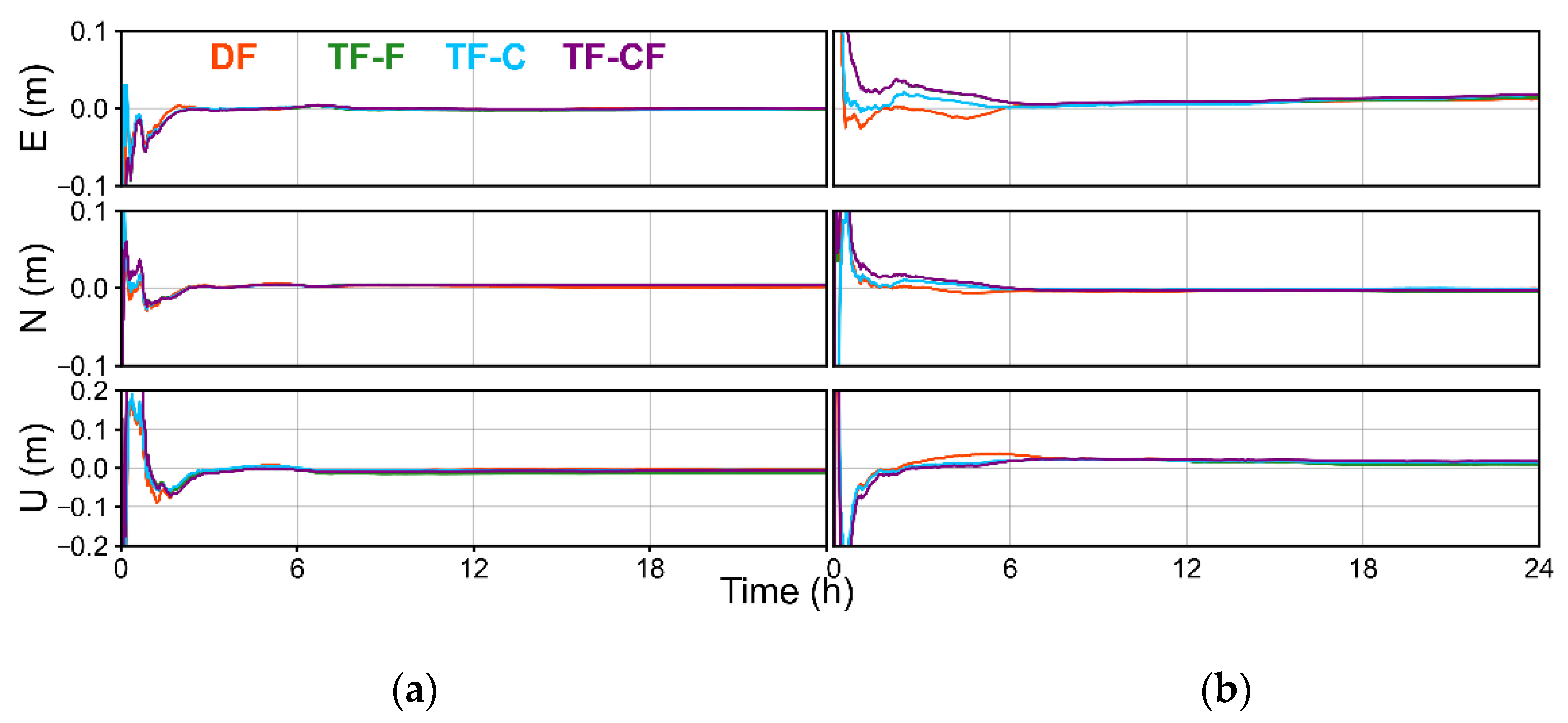
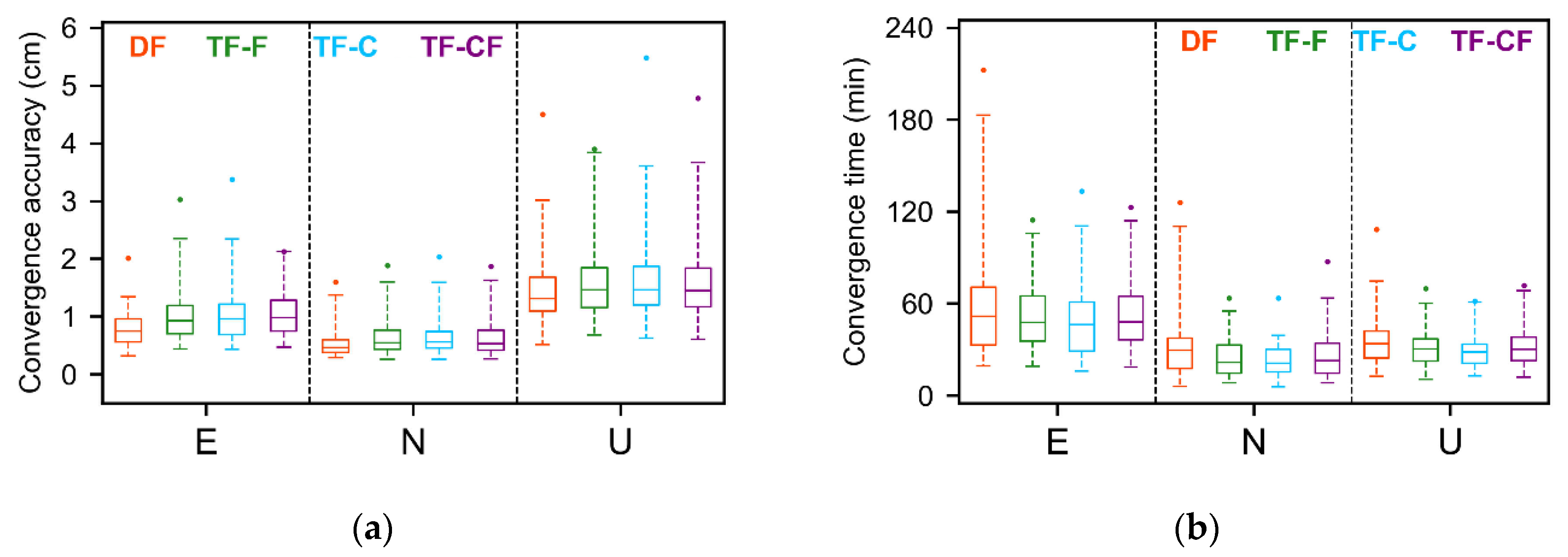
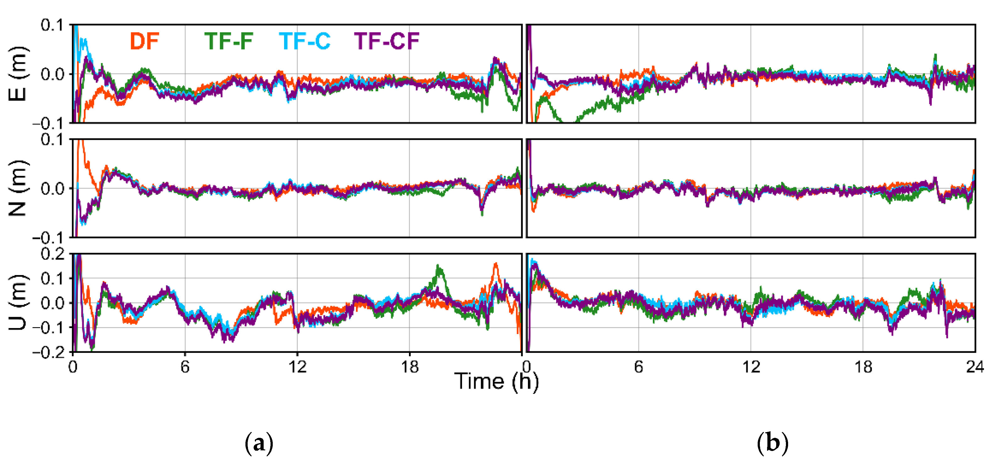
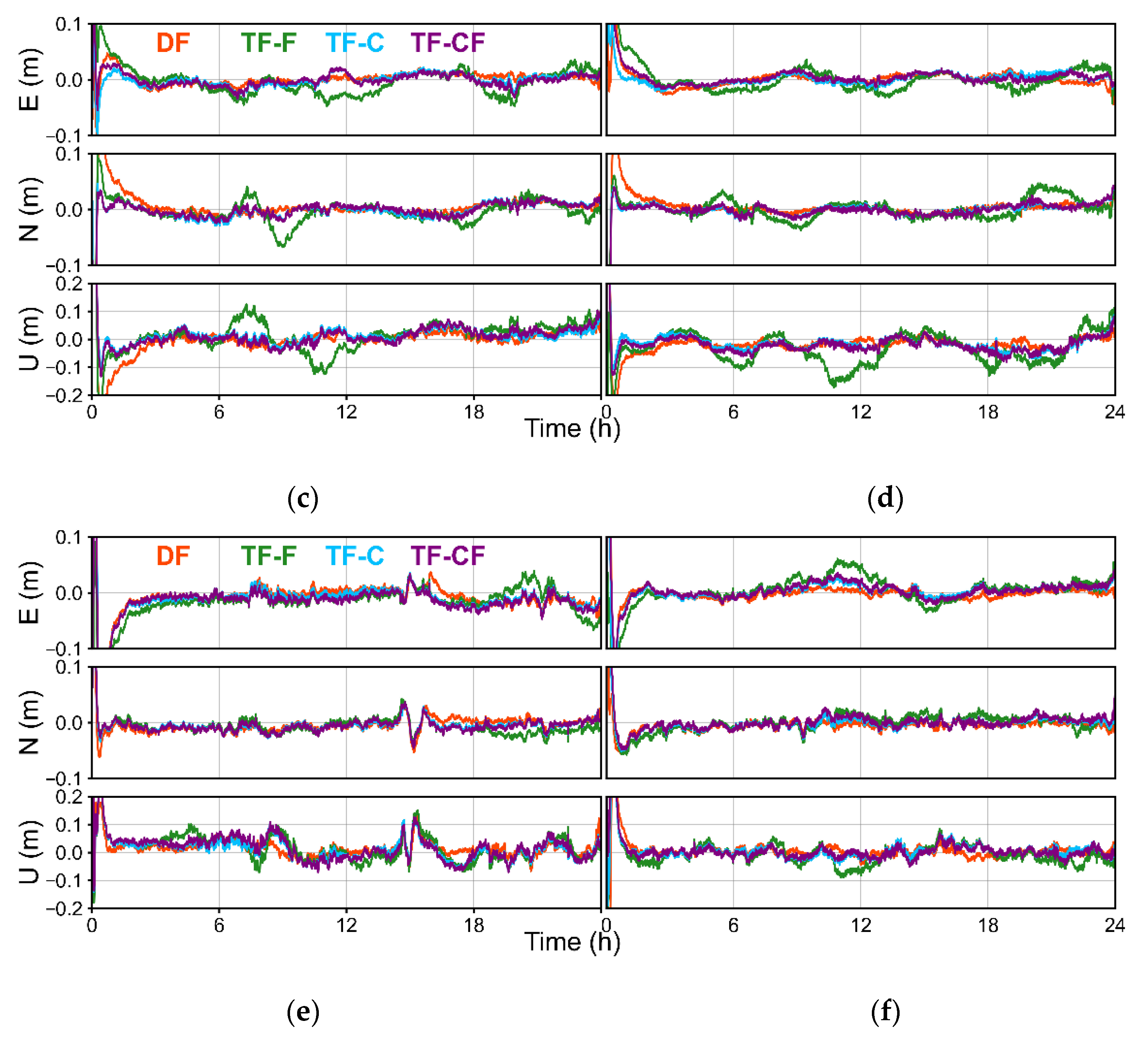
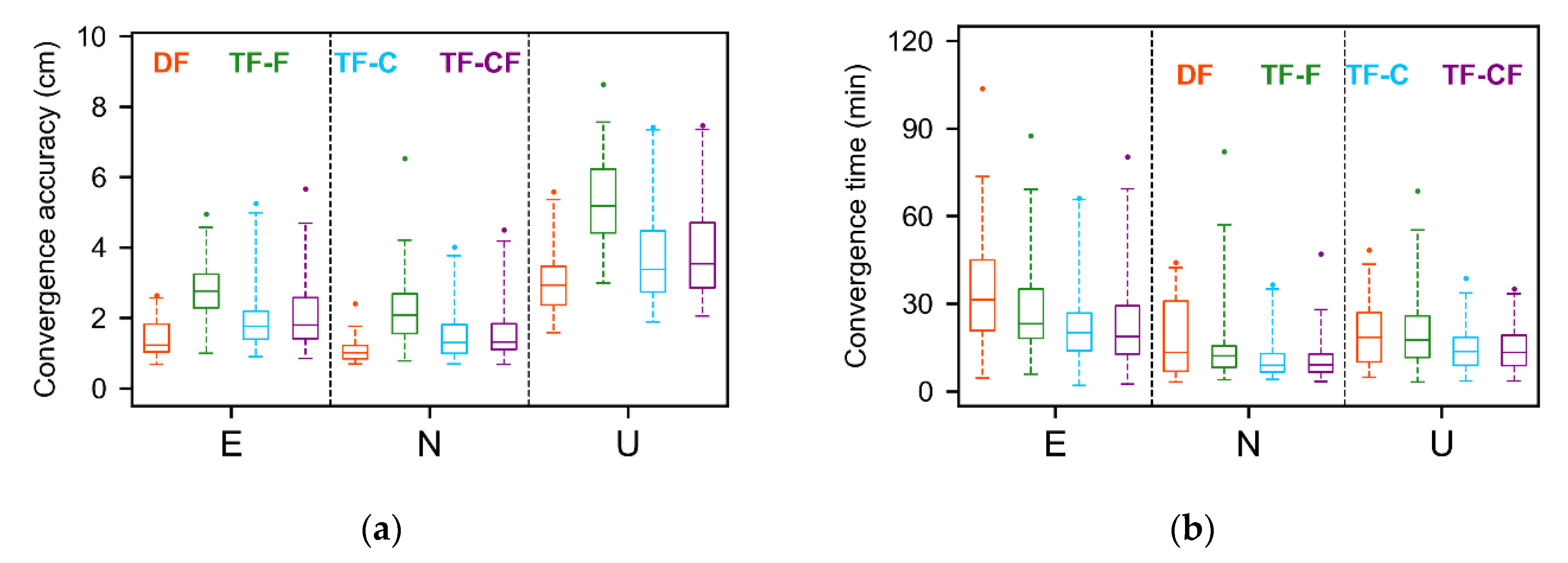
This section describes the BDS/GPS dual-system experiment with the same data sources as described in Section 3.1. The PPP models are the DF, TF-F, TF-C and TF-CF models. In the TF-CF model, the GPS is the first system, and the BDS is the second system. The other data-processing strategies are consistent with those given in Table 3.

3.3.1. Static Mode

This section gives four BDS/GPS static PPP models for positioning. Figure 7 shows the static positioning error curves of stations CUSV, DGAR, GAMG, MIZU, SEYG and MOBS on DOY121. The positioning accuracy of the TF-F model for the CUSV and DGAR stations is less than their median, while it is greater than their median for the GAMG, MIZU, SEYG and MOBS stations. It can be observed that the DF and TF-F models perform slightly worse in the convergence process compared to the other three frequency models. After convergence in the E, N and U directions, the positioning error curves of the four PPP models basically coincide.
Figure 8 shows that, except for the TF-F model, the positioning accuracy of the stations does not improve significantly with the addition of the third frequency [34], but the convergence time is slightly reduced. Table 6 demonstrates that the positioning accuracy is better than 1.0 cm, except for the TF-F model’s U direction, and better than 1.5 cm for the TF-F model’s U direction. In terms of convergence time, the convergence time of the TF-CF model is improved by 18.1%, 9.7% and 12.1% in the E, N and U directions, respectively. The convergence time of TF-C model is the shortest among the triple-frequency PPP models. It is 28.43, 11.61 and 16.68 min in the E, N and U directions with improvements of 23.5%, 13.6% and 19.8%, respectively.
In contrast to the experiment above, in the dual-system static PPP experiment, ignoring the GPS PIFCB had a slight effect on the PPP results; this is because the BDS plays a major role in the PPP process, as the BDS can ignore the PIFCB [43].

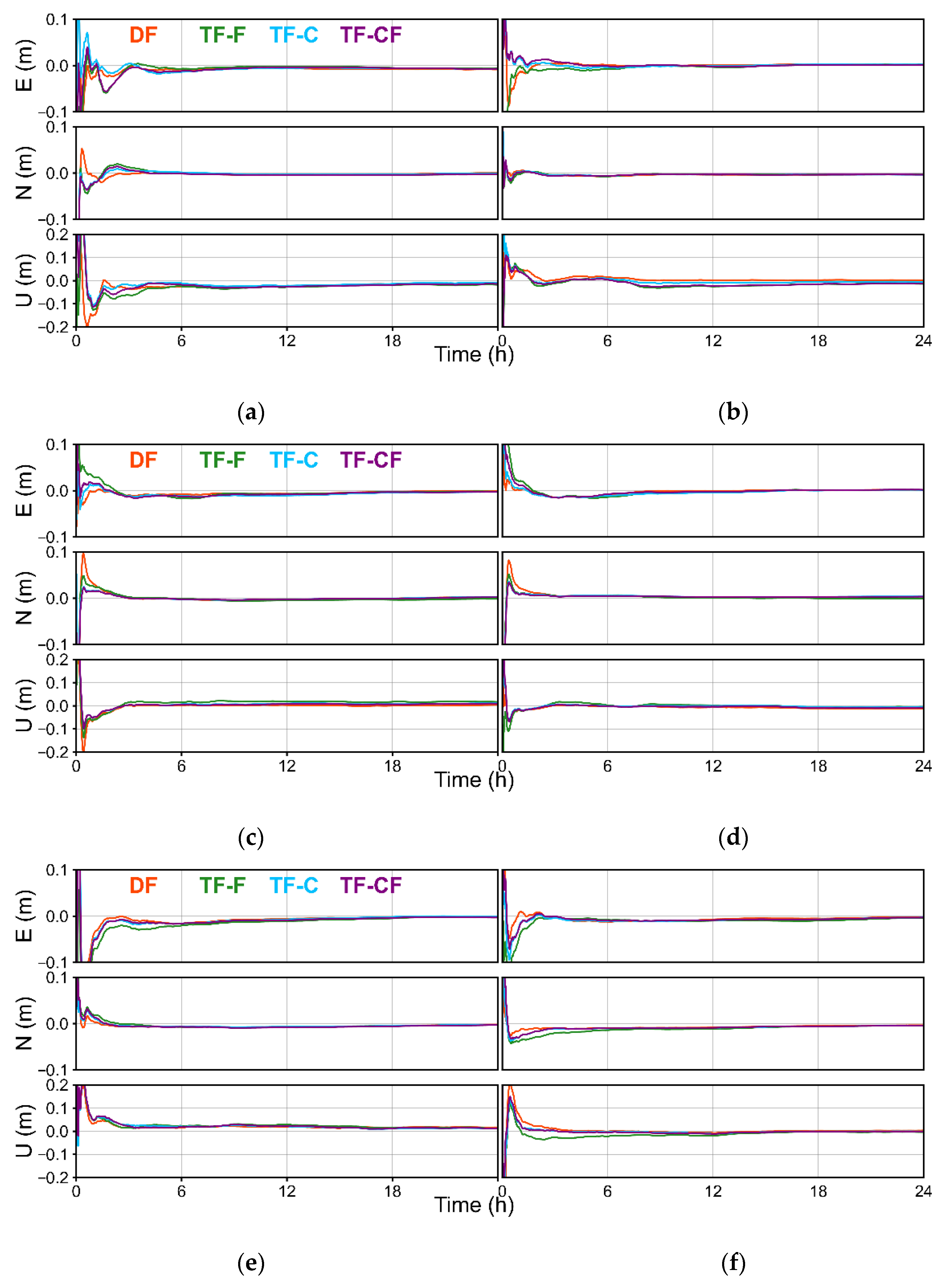
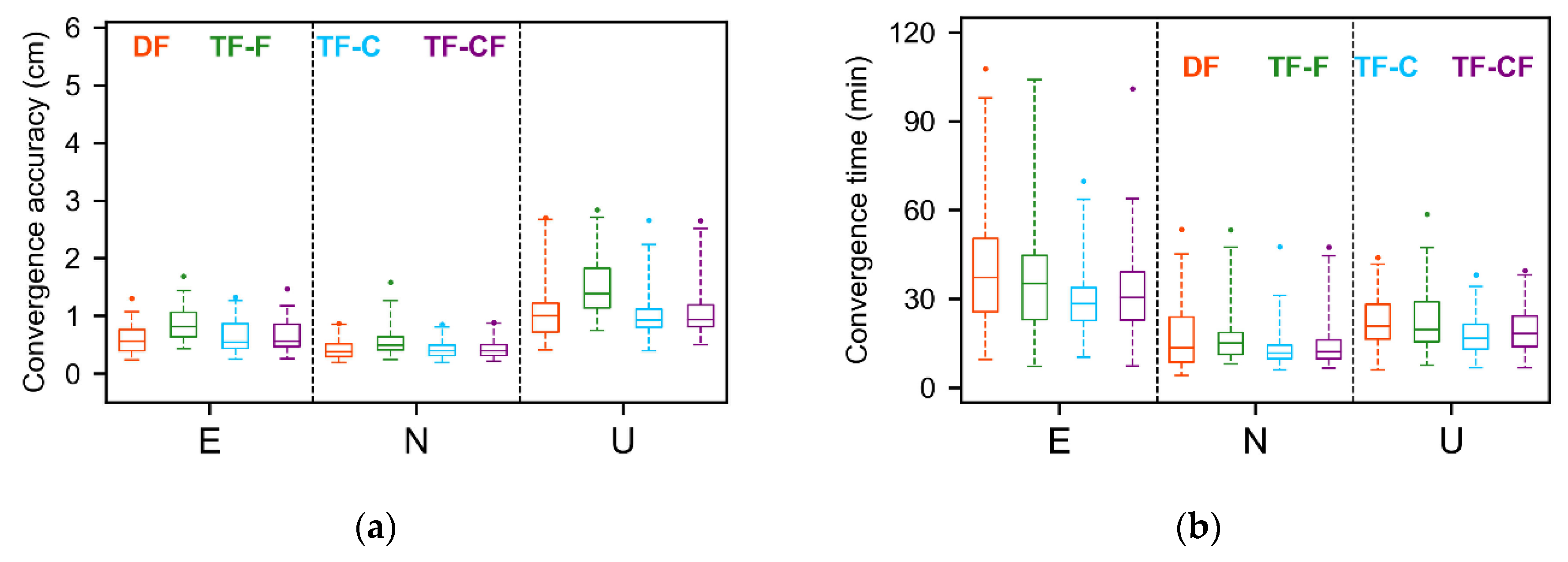
3.3.2. Kinematic Mode

This section describes four BDS/GPS kinematic PPP models for positioning. In Figure 9, the kinematic PPP results differ from the BDS/GPS static PPP results. Ignoring the GPS PIFCB significantly affects the convergence time. Additionally, the triple-frequency PPP models in addition to the TF-F model make the convergence much faster than the DF PPP model.
Figure 10 and Table 7 show that the positioning performance of the models is similar, except for the TF-F model, where the horizontal positioning accuracy is better than 2.0 cm and the U-direction accuracy is better than 4.0 cm. In terms of convergence time, the TF-C model is improved by 46.2%, 33.5% and 35.1% in the E, N and U directions, respectively, and the TF-CF model is improved by 49.6%, 32.4% and 36.1%, respectively.

4. Conclusions

This study focuses on the precision modeling of the dual-system triple-frequency IF1213 PPP based on BDS/GPS triple-frequency observations. The TF-C model is able to estimate the IFCB. This was deduced by considering the time-varying part of the phase hardware bias of the receiver and satellite. The TF-CF model is able to estimate the IFCB of the first GNSS. This was deduced by considering that the time-varying part of the phase bias of the receiver and the satellite in the first system, and the second one can be ignored. The advantage of the TF-C model is that it does not require the DCB product and IFCB product to correct the corresponding deviation terms. The disadvantage is that it has a large number of parameters to be estimated, which can reduce the degrees of freedom of the observation equation and lead to an increased convergence time when applied to GPS. The reliability of the deduced models was demonstrated using static PPP experiments for a single system. GPS PPP experiments demonstrated the reliability of the models, except for the TF-CF model, and the fact that GPS PIFCB has a bad influence on the GPS PPP. The BDS PPP experiments demonstrated the reliability of the TF-CF model and the negligible effect of the BDS-2 PIFCB when BDS-2 and BDS-3 are used as the BDS.
Using one week of observation from 60 stations provided by the MGEX of the IGS organization, we conducted a BDS/GPS dual-system static and kinematic experiment. The results show that the GPS PIFCB had less of an influence in the static experiment, while the influence was greater in the kinematic experiment. The performance of the DF, TF-C and TF-CF models is similar; the positioning accuracy is better than 1.0 cm in the three directions in the static experiment, and in the kinematic experiment, the horizontal positioning accuracy is better than 2.0 cm, while the U directional positioning accuracy is better than 4.0 cm. The addition of third-frequency data does not significantly improve the positioning accuracy [34], but the convergence time is reduced. Compared with the DF model, the TF-C model improves the convergence time by approximately 23.5%, 13.6% and 19.8% in the E, N and U directions, respectively, and the TF-CF model improves by approximately 18.1%, 9.7% and 12.1%, respectively, in the static experiment. In the kinematic experiment, the TF-C model improves by approximately 46.2%, 33.5% and 35.1% in the E, N and U directions, respectively, and the TF-CF model improves by approximately 49.6%, 32.4% and 36.1%, respectively. The positioning performance of the TF-C model is slightly better than that of the TF-CF model, probably because the IFCB parameters in the TF-C model can absorb the residuals. However, one should be aware that the positioning performance of IF1213 PPP models is limited due to the limitations of the float ambiguity solution. Therefore, we will focus on finding a multi-frequency solution to integer ambiguity in the future.
For dual-system PPP based on BDS/GPS observations, the TF-C model is the most rigorous; therefore, the TF-C model is recommended.

Author Contributions

Conceptualization, Z.W. and R.W.; methodology, R.W.; software, R.W.; validation, Z.W., R.W. and Y.W.; formal analysis, R.W.; investigation, Z.W. and Y.W.; resources, Z.W. and C.H.; data curation, C.H. and B.L.; writing—original draft preparation, R.W.; writing—review and editing, Z.W., R.W., Y.W., C.H. and B.L.; visualization, R.W.; supervision, Z.W. and C.H.; project administration, Z.W. and Y.W.; funding acquisition, Z.W. All authors have read and agreed to the published version of the manuscript.

Funding

This research was funded by Natural Science Foundation of Jiangsu Province, No. BK20181361; Natural Science Foundation of Jiangsu Province, No. BK20191342, the Natural Science Foundation of Anhui Colleges (Grant No. KJ2020A0310) and Anhui Natural Science Foundation (Grant No. 2108085QD173).

Data Availability Statement

The observation data and precise products used in the research are available on the FTP of Wuhan University (ftp://igs.gnsswhu.cn/pub/, accessed on 20 May 2022). The GPS satellite PIFCB products were obtained from iGMAS Innovation Application Center (http://igmas.users.sgg.whu.edu.cn/products/download/directory/products/upd/2022/, accessed on 20 May 2022).

Acknowledgments

The authors gratefully acknowledge WUM for providing the observation data, the precise products and iGMAS Innovation Application Center for providing GPS satellite PIFCB products.

Conflicts of Interest

The authors declare no conflict of interest.

References

  1. Zumberge, J.F.; Heflin, M.B.; Jefferson, D.C.; Watkins, M.M.; Webb, F.H. Precise point positioning for the efficient and robust analysis of GPS data from large networks. J. Geophys. Res. Solid Earth 1997, 102, 5005–5017. [Google Scholar] [CrossRef]
  2. Malys, S.; Jensen, P.A. Geodetic point positioning with GPS carrier beat phase data from the CASA UNO Experiment. Geophys. Res. Lett. 1990, 17, 651–654. [Google Scholar] [CrossRef]
  3. Deo, M.; El-Mowafy, A. Triple-frequency GNSS models for PPP with float ambiguity estimation: Performance comparison using GPS. Surv. Rev. 2018, 50, 249–261. [Google Scholar] [CrossRef]
  4. Xiao, G.R.; Li, P.; Gao, Y.; Heck, B. A Unified Model for Multi-Frequency PPP Ambiguity Resolution and Test Results with Galileo and BeiDou Triple-Frequency Observations. Remote Sens. 2019, 11, 116. [Google Scholar] [CrossRef]
  5. Liu, G.; Guo, F.; Wang, J.; Du, M.Y.; Qu, L.Z. Triple-Frequency GPS Un-Differenced and Uncombined PPP Ambiguity Resolution Using Observable-Specific Satellite Signal Biases. Remote Sens. 2020, 12, 2310. [Google Scholar] [CrossRef]
  6. Naciri, N.; Bisnath, S. An uncombined triple-frequency user implementation of the decoupled clock model for PPP-AR. J. Geod. 2021, 95, 1–17. [Google Scholar] [CrossRef]
  7. Tsai, Y.-H.; Yang, W.-C.; Chang, F.-R.; Ma, C.-L. Using multi-frequency for GPS positioning and receiver autonomous integrity monitoring. In Proceedings of the 2004 IEEE International Conference on Control Applications, Taipei, Taiwan, 2–4 September 2004; pp. 205–210. [Google Scholar]
  8. Zhao, Q.L.; Sun, B.Z.; Dai, Z.Q.; Hu, Z.G.; Shi, C.; Liu, J.N. Real-time detection and repair of cycle slips in triple-frequency GNSS measurements. GPS Solut. 2015, 19, 381–391. [Google Scholar] [CrossRef]
  9. Gu, X.Y.; Zhu, B.C. Detection and Correction of Cycle Slip in Triple-Frequency GNSS Positioning. IEEE Access 2017, 5, 12584–12595. [Google Scholar] [CrossRef]
  10. Li, P.; Jiang, X.; Zhang, X.; Ge, M.; Schuh, H. GPS + Galileo + BeiDou precise point positioning with triple-frequency ambiguity resolution. GPS Solut. 2020, 24, 78. [Google Scholar] [CrossRef]
  11. Spits, J.; Warnant, R. Total electron content monitoring using triple frequency GNSS data: A three-step approach. J. Atmos. Sol. Terr. Phys. 2008, 70, 1885–1893. [Google Scholar] [CrossRef]
  12. Montenbruck, O.; Hauschild, A.; Steigenberger, P.; Langley, R. Three’s the challenge: A close look at GPS SVN62 triple-frequency signal combinations finds carrier-phase variations on the new L5. GPS World 2010, 21, 8–19. [Google Scholar]
  13. Montenbruck, O.; Hugentobler, U.; Dach, R.; Steigenberger, P.; Hauschild, A. Apparent clock variations of the Block IIF-1 (SVN62) GPS satellite. GPS Solut. 2012, 16, 303–313. [Google Scholar] [CrossRef]
  14. Pan, L.; Zhang, X.; Guo, F.; Liu, J. GPS inter-frequency clock bias estimation for both uncombined and ionospheric-free combined triple-frequency precise point positioning. J. Geod. 2019, 93, 473–487. [Google Scholar] [CrossRef]
  15. Steigenberger, P.; Hauschild, A.; Montenbruck, O.; Rodriguez-Solano, C.; Hugentobler, U. Orbit and Clock Determination of QZS-1 Based on the CONGO Network. Navigation 2013, 60, 31–40. [Google Scholar] [CrossRef]
  16. Cai, C.S.; He, C.; Santerre, R.; Pan, L.; Cui, X.Q.; Zhu, J.J. A comparative analysis of measurement noise and multipath for four constellations: GPS, BeiDou, GLONASS and Galileo. Surv. Rev. 2016, 48, 287–295. [Google Scholar] [CrossRef]
  17. Montenbruck, O.; Hauschild, A.; Steigenberger, P.; Hugentobler, U.; Teunissen, P.; Nakamura, S. Initial assessment of the COMPASS/BeiDou-2 regional navigation satellite system. GPS Solut. 2013, 17, 211–222. [Google Scholar] [CrossRef]
  18. Zhao, Q.; Wang, G.X.; Liu, Z.Z.; Hu, Z.G.; Dai, Z.Q.; Liu, J.N. Analysis of BeiDou Satellite Measurements with Code Multipath and Geometry-Free Ionosphere-Free Combinations. Sensors 2016, 16, 123. [Google Scholar] [CrossRef]
  19. Fan, L.; Wang, C.; Guo, S.; Fang, X.; Jing, G.; Shi, C. GNSS satellite inter-frequency clock bias estimation and correction based on IGS clock datum: A unified model and result validation using BDS-2 and BDS-3 multi-frequency data. J. Geod. 2021, 95, 135. [Google Scholar] [CrossRef]
  20. Gong, X.; Gu, S.; Lou, Y.; Zheng, F.; Yang, X.; Wang, Z.; Liu, J. Research on empirical correction models of GPS Block IIF and BDS satellite inter-frequency clock bias. J. Geod. 2020, 94, 36. [Google Scholar] [CrossRef]
  21. Pan, L.; Zhang, X.H.; Li, X.X.; Liu, J.N.; Li, X. Characteristics of inter-frequency clock bias for Block IIF satellites and its effect on triple-frequency GPS precise point positioning. GPS Solut. 2017, 21, 811–822. [Google Scholar] [CrossRef]
  22. Lu, X.F.; Zhang, S.L.; Bao, Y.C. A New Method of Ambiguity Resolution for Triple-Frequency GPS PPP. ITM Web Conf. 2016, 7, 01010. [Google Scholar] [CrossRef] [Green Version]
  23. Guo, F.; Zhang, X.H.; Wang, J.L.; Ren, X.D. Modeling and assessment of triple-frequency BDS precise point positioning. J. Geod. 2016, 90, 1223–1235. [Google Scholar] [CrossRef]
  24. Pan, L.; Zhang, X.H.; Liu, J.N. A comparison of three widely used GPS triple-frequency precise point positioning models. GPS Solut. 2019, 23, 1–13. [Google Scholar] [CrossRef]
  25. Cai, C.S.; Gao, Y.; Pan, L.; Zhu, J.J. Precise point positioning with quad-constellations: GPS, BeiDou, GLONASS and Galileo. Adv. Space Res. 2015, 56, 133–143. [Google Scholar] [CrossRef]
  26. Ren, X.D.; Zhang, X.H.; Xie, W.L.; Zhang, K.K.; Yuan, Y.Q.; Li, X.X. Global Ionospheric Modelling using Multi-GNSS: BeiDou, Galileo, GLONASS and GPS. Sci. Rep. 2016, 6, 1–11. [Google Scholar] [CrossRef]
  27. Gao, X.; Dai, W.J.; Song, Z.Y.; Cai, C.S. Reference satellite selection method for GNSS high-precision relative positioning. Geod. Geodyn. 2017, 8, 125–129. [Google Scholar] [CrossRef]
  28. Pan, L.; Zhang, X.H.; Liu, J.N.; Li, X.X.; Li, X. Performance Evaluation of Single-frequency Precise Point Positioning with GPS, GLONASS, BeiDou and Galileo. J. Navig. 2017, 70, 465–482. [Google Scholar] [CrossRef]
  29. Li, X.X.; Li, X.; Liu, G.G.; Feng, G.L.; Yuan, Y.Q.; Zhang, K.K.; Ren, X.D. Triple-frequency PPP ambiguity resolution with multi-constellation GNSS: BDS and Galileo. J. Geod. 2019, 93, 1105–1122. [Google Scholar] [CrossRef]
  30. Hu, C. An Investigation of Key Technologies Related to Combining BDS-2 and BDS-3 Observations in Data Processing; China University of Mining and Technology: Xuzhou, China, 2020. [Google Scholar]
  31. Leick, A.; Rapoport, L.; Tatarnikov, D. GPS Satellite Surveying, 1st ed.; John Wiley & Sons, Ltd.: Hoboken, NJ, USA, 2015. [Google Scholar]
  32. Liu, T.; Zhang, B.; Yuan, Y.; Li, Z.; Wang, N. Multi-GNSS triple-frequency differential code bias (DCB) determination with precise point positioning (PPP). J. Geod. 2019, 93, 765–784. [Google Scholar] [CrossRef]
  33. Chen, L.; Li, M.; Zhao, Y.; Hu, Z.; Zheng, F.; Shi, C. Multi-GNSS real-time precise clock estimation considering the correction of inter-satellite code biases. GPS Solut. 2021, 25, 32. [Google Scholar] [CrossRef]
  34. Zhou, F.; Xu, T. Modeling and assessment of GPS/BDS/Galileo treple-frequency precise point positioning. Acta Geod. Cartogr. Sin. 2021, 50, 61–70. [Google Scholar]
  35. Li, P.; Zhang, X.H.; Ge, M.R.; Schuh, H. Three-frequency BDS precise point positioning ambiguity resolution based on raw observables. J. Geod. 2018, 92, 1357–1369. [Google Scholar] [CrossRef] [Green Version]
  36. Zhou, F.; Dong, D.; Li, P.; Li, X.; Schuh, H. Influence of stochastic modeling for inter-system biases on multi-GNSS undifferenced and uncombined precise point positioning. GPS Solut. 2019, 23, 59. [Google Scholar] [CrossRef]
  37. Schmid, R.; Steigenberger, P.; Gendt, G.; Ge, M.; Rothacher, M. Generation of a consistent absolute phase-center correction model for GPS receiver and satellite antennas. J. Geod. 2007, 81, 781–798. [Google Scholar] [CrossRef]
  38. Wu, J.-T.; Wu, S.-C.; Hajj, G.; Bertiger, W.; Lichten, S.M. Effects of antenna orientation on GPS carrier phase. Astrodynamics 1991 1992, 91–98. [Google Scholar]
  39. Saastamoinen, J. Contributions to the theory of atmospheric refraction. Bulletin Géodésique (1946–1975) 1973, 107, 13–34. [Google Scholar] [CrossRef]
  40. Petit, G.; Luzum, B.; Conventions, I. IERS Conventions (2010); Bundesamts für Kartographie und Geodäsie: Frankfurt am Main, Germany, 2010. [Google Scholar]
  41. Ashby, N. Relativity in the Global Positioning System. Living Rev. Relativ. 2003, 6, 1. [Google Scholar] [CrossRef] [PubMed]
  42. Fan, L.; Shi, C.; Li, M.; Wang, C.; Zheng, F.; Jing, G.; Zhang, J. GPS satellite inter-frequency clock bias estimation using triple-frequency raw observations. J. Geod. 2019, 93, 2465–2479. [Google Scholar] [CrossRef]
  43. Chen, Y.; Mi, J.; Gu, S.; Li, B.; Li, H.; Yang, L.; Pang, Y. GPS, BDS-3, and Galileo Inter-Frequency Clock Bias Deviation Time-Varying Characteristics and Positioning Performance Analysis. Remote Sens. 2022, 14, 3991. [Google Scholar] [CrossRef]
Figure 1. Geographical distribution of the 60 selected MGEX stations.
Remotesensing 14 04509 g001
Figure 2. Positioning error of the four GPS static PPP models (DOY127, 2022). The stations are (a) KOUR and (b) WIND, respectively.
Remotesensing 14 04509 g002
Figure 3. Variation in the PIFCB values from the GPS satellites at the KOUR station.
Remotesensing 14 04509 g003
Figure 4. Positioning accuracy and convergence time distribution of the four GPS static PPP models. (a) Convergence accuracy. (b) Convergence time.
Remotesensing 14 04509 g004
Figure 5. Positioning error of the four BDS static PPP models (DOY127, 2022). The stations are (a) SUTH and (b) ULAB, respectively.
Remotesensing 14 04509 g005
Figure 6. Positioning accuracy and convergence time distribution of the four BDS static PPP models. (a) Convergence accuracy. (b) Convergence time.
Remotesensing 14 04509 g006
Figure 7. Positioning error of the four BDS/GPS static PPP models (DOY121, 2022). The stations are (a) CUSV, (b) DGAR, (c) GAMG, (d) MIZU (e) SEYG and (f) MOBS, respectively.
Remotesensing 14 04509 g007
Figure 8. Positioning accuracy and convergence time distribution of the four BDS/GPS static PPP models. (a) Convergence accuracy. (b) Convergence time.
Remotesensing 14 04509 g008
Figure 9. Positioning error of the four BDS/GPS kinematic PPP models (DOY121, 2022). The stations are (a) CUSV, (b) DGAR, (c) GAMG, (d) MIZU, (e) SEYG and (f) MOBS, respectively.
Remotesensing 14 04509 g009aRemotesensing 14 04509 g009b
Figure 10. Positioning accuracy and convergence time distribution of the four BDS/GPS kinematic PPP models. (a) Convergence accuracy. (b) Convergence time.
Remotesensing 14 04509 g010
Table 1. BDS/GPS frequency number.
NumberGPSBDS-2BDS-3
1L1 (1575.42)B1I (1561.01)B1I (1561.01)
2L2 (1227.60)B3I (1268.52)B3I (1268.52)
3L5 (1176.45)B2I (1207.14)B1C (1575.42)
Table 2. BDS/GPS satellites transmitting triple frequency signals.
SystemPRNOrbit Type
GPSG01, G03, G04, G06, G08, G09, G10, G14, G18, G23, G24, G25, G26, G27, G30, G32.Medium Earth Orbit (MEO)
BDS-2C01, C02, C03, C04, C05;Geostationary Earth Orbit (GEO)
C06, C07, C08, C09, C10, C13, C16;Inclined Geo-Synchronous Orbit (IGSO)
C11, C12, C14;MEO
BDS-3C19, C20, C21, C22, C23, C24, C25, C26, C27, C28, C29, C30, C32, C33, C34, C35, C36, C37, C41, C42, C43, C44, C45, C46;MEO
C38, C39, C40.IGSO
Table 3. Data-processing strategies.
ItemsStrategy
ModelDF, TF-C, TF-F, TF-CF, TF-FP(GPS)
Satellite elevation mask15°
EstimatorKalman filter
Weighting scheme Elevation-dependent weight; 0.003 m and 0.3 m for raw phase and code, respectively
PCO/PCVigs14_2196.atx according to Schmid et al. [37]
Phase windupCorrected [38]
Satellite DCB corrections Corrected with MGEX DCB products except TF-C model
Satellite orbit and clock Products from WUM
Tropospheric delayZenith Hydrostatic Delays (ZHD) are corrected using the Saastamoinen model, and Zenith Wet Delays (ZWD) are estimated using random walk [39]
Tide effectSolid Earth, pole and ocean tide [40]
Relativistic effectCorrected [41]
Station coordinates Static: estimated using constants; kinematic: estimated using white noise process
Receiver clockEstimated using white noises
Receiver inter-frequency biasEstimated using random walk
Inter-frequency clock biasEstimated using random walk
AmbiguityEstimated using a constant
Table 4. Statistics on the positioning results of the four GPS static PPP models.
ModelConvergence Accuracy (CM)Convergence Time (Min)
ENUENU
DF0.610.371.2630.8610.1720.14
TF-F1.560.943.0086.3640.6454.43
TF-C0.660.421.1236.9314.0022.21
TF-FP0.860.452.0184.2538.2151.79
Table 5. Statistics on the positioning results of the four BDS static PPP models.
ModelConvergence Accuracy (CM)Convergence Time (Min)
ENUENU
DF0.740.461.3151.6429.5733.64
TF-F0.930.541.4647.5921.6930.36
TF-C0.960.561.4646.1421.0028.29
TF-CF0.980.531.4447.8922.7529.96
Table 6. Statistics on the positioning results of the four BDS/GPS static PPP models.
ModelConvergence Accuracy (CM)Convergence Time (Min)
ENUENU
DF0.560.381.0037.1813.4320.80
TF-F0.810.491.3935.1815.0419.54
TF-C0.540.390.9328.4311.6116.68
TF-CF0.560.390.9330.4612.1218.29
Table 7. Statistics on the positioning results of the four BDS/GPS kinematic PPP models.
ModelConvergence Accuracy (CM)Convergence Time (Min)
ENUENU
DF1.231.012.9331.2413.3318.39
TF-F2.752.085.1723.0712.1317.47
TF-C1.751.293.3720.028.9313.50
TF-CF1.791.313.5318.749.0813.29
Publisher’s Note: MDPI stays neutral with regard to jurisdictional claims in published maps and institutional affiliations.

