

Evaluating and Analyzing the Potential of the Gaofen-3 SAR Satellite for Landslide Monitoring

 , ,
, ,
Abstract
:
1. Introduction
2. Study Area and Dataset
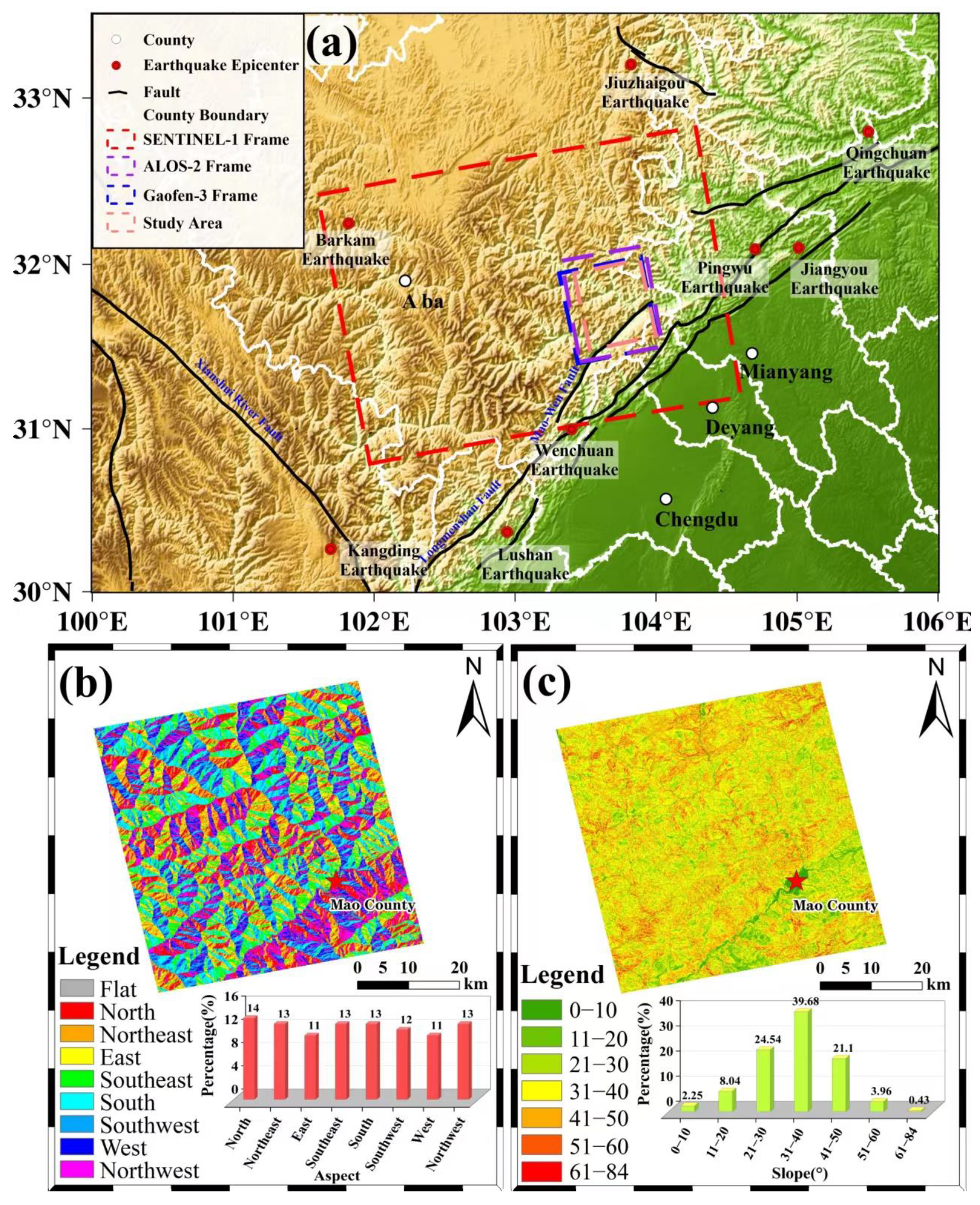
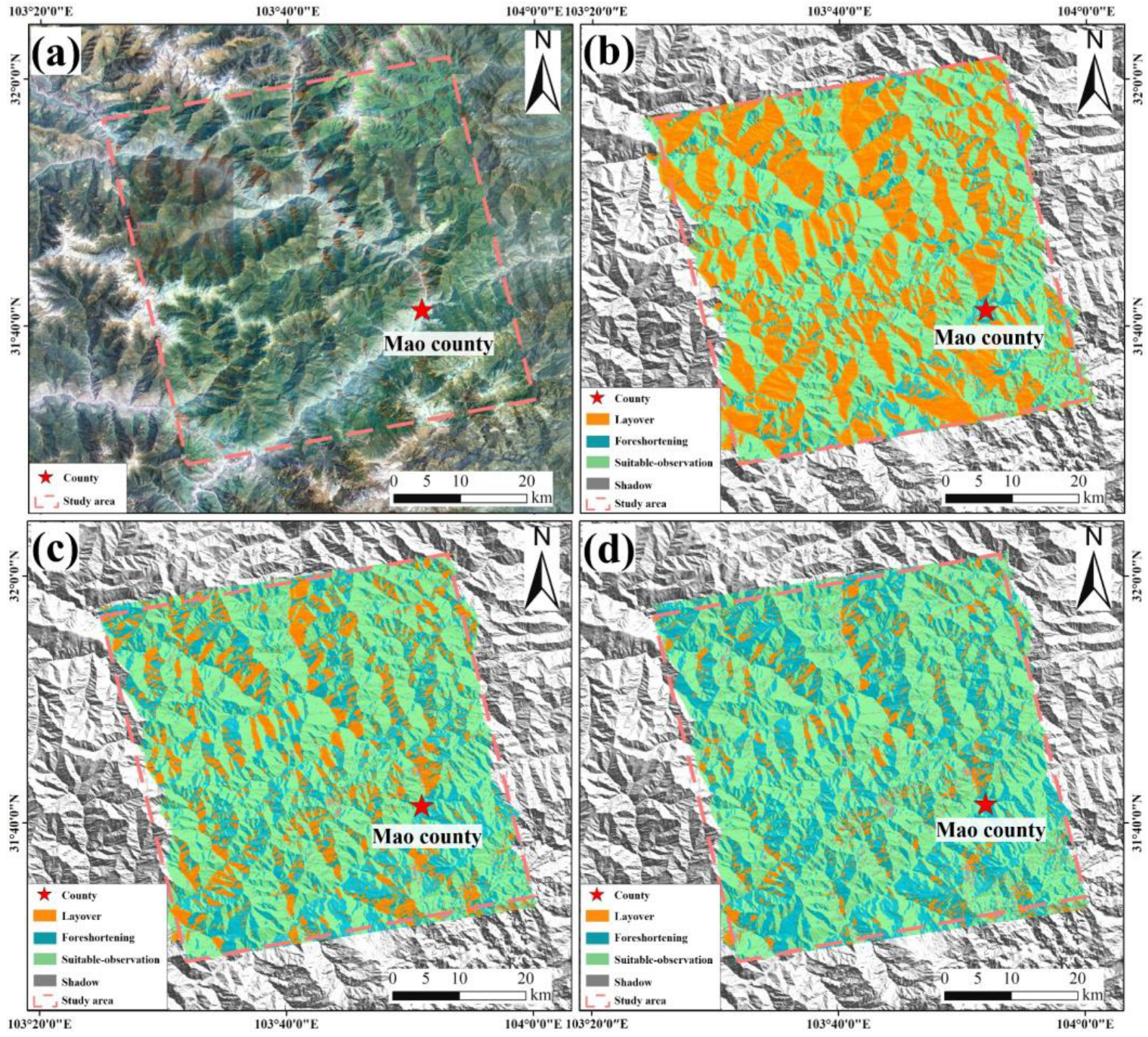
2.1. Overview of the Study Area
2.2. Dataset
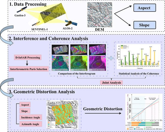
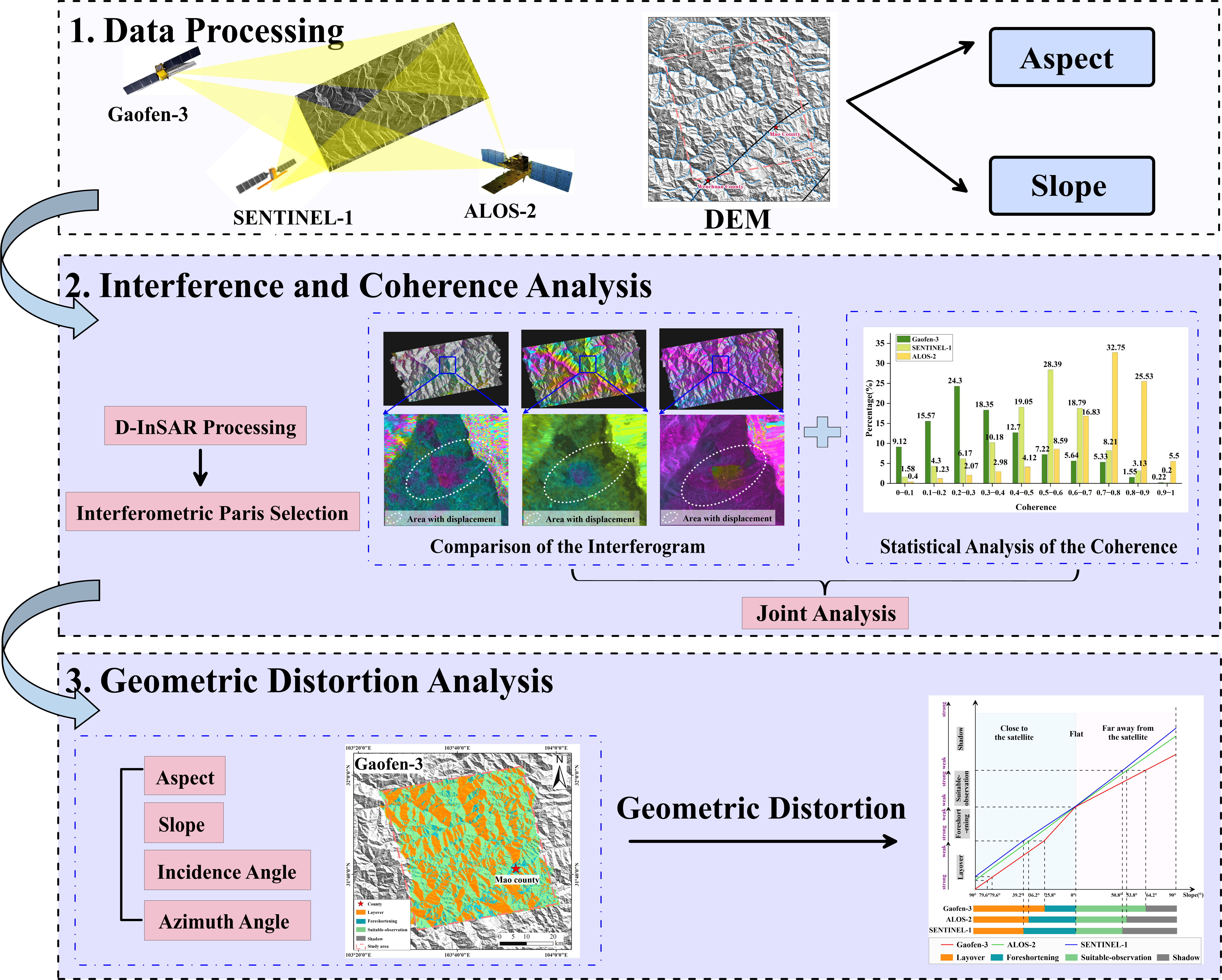
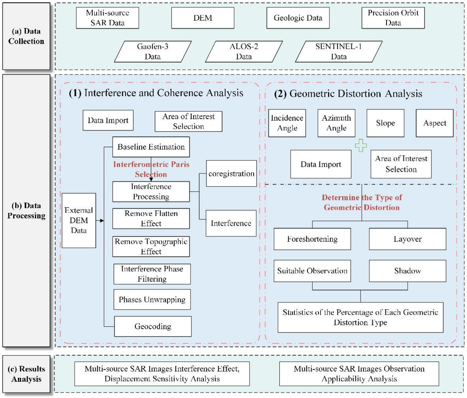
3. Methodology
4. Result and Discussion
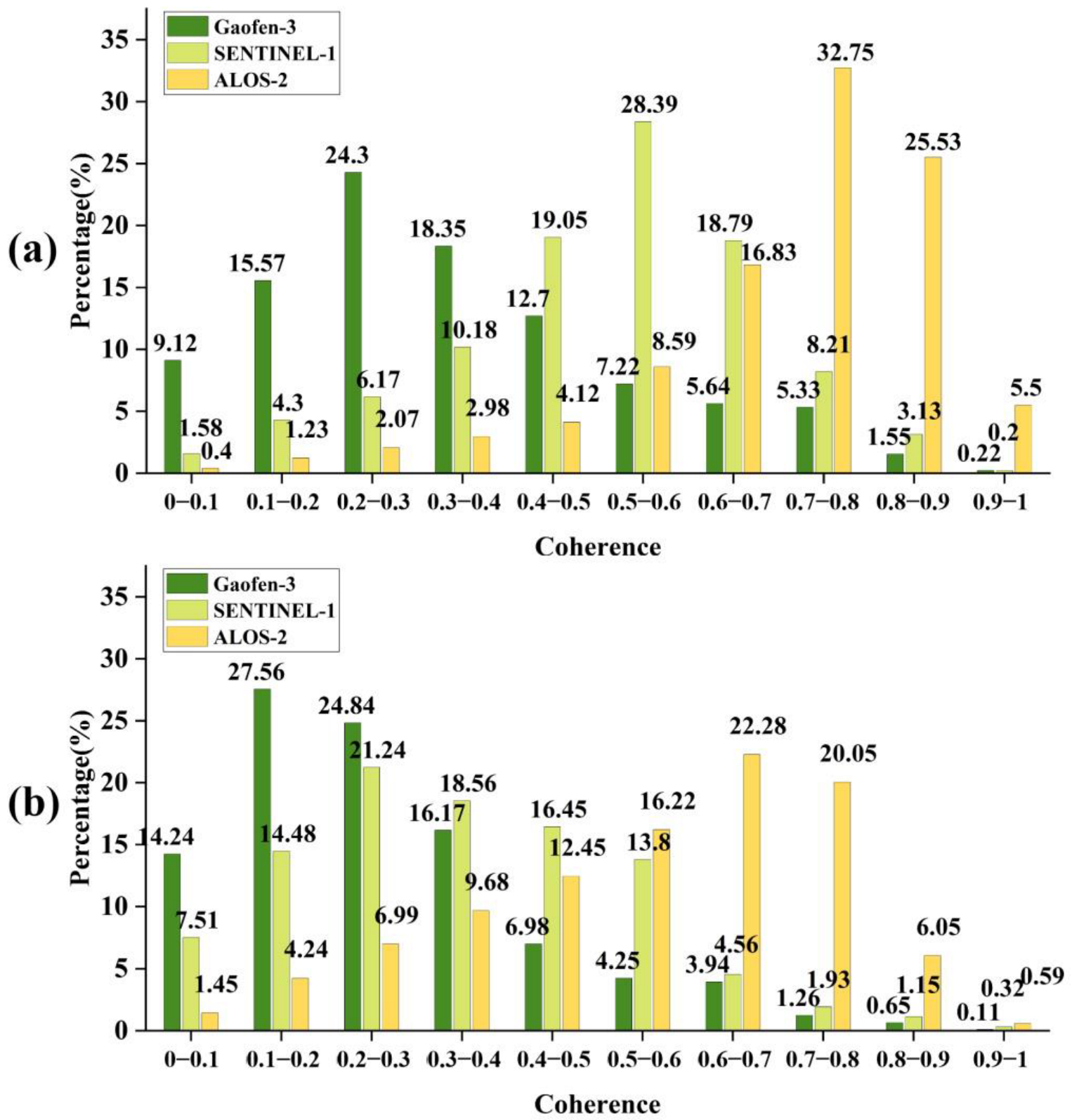
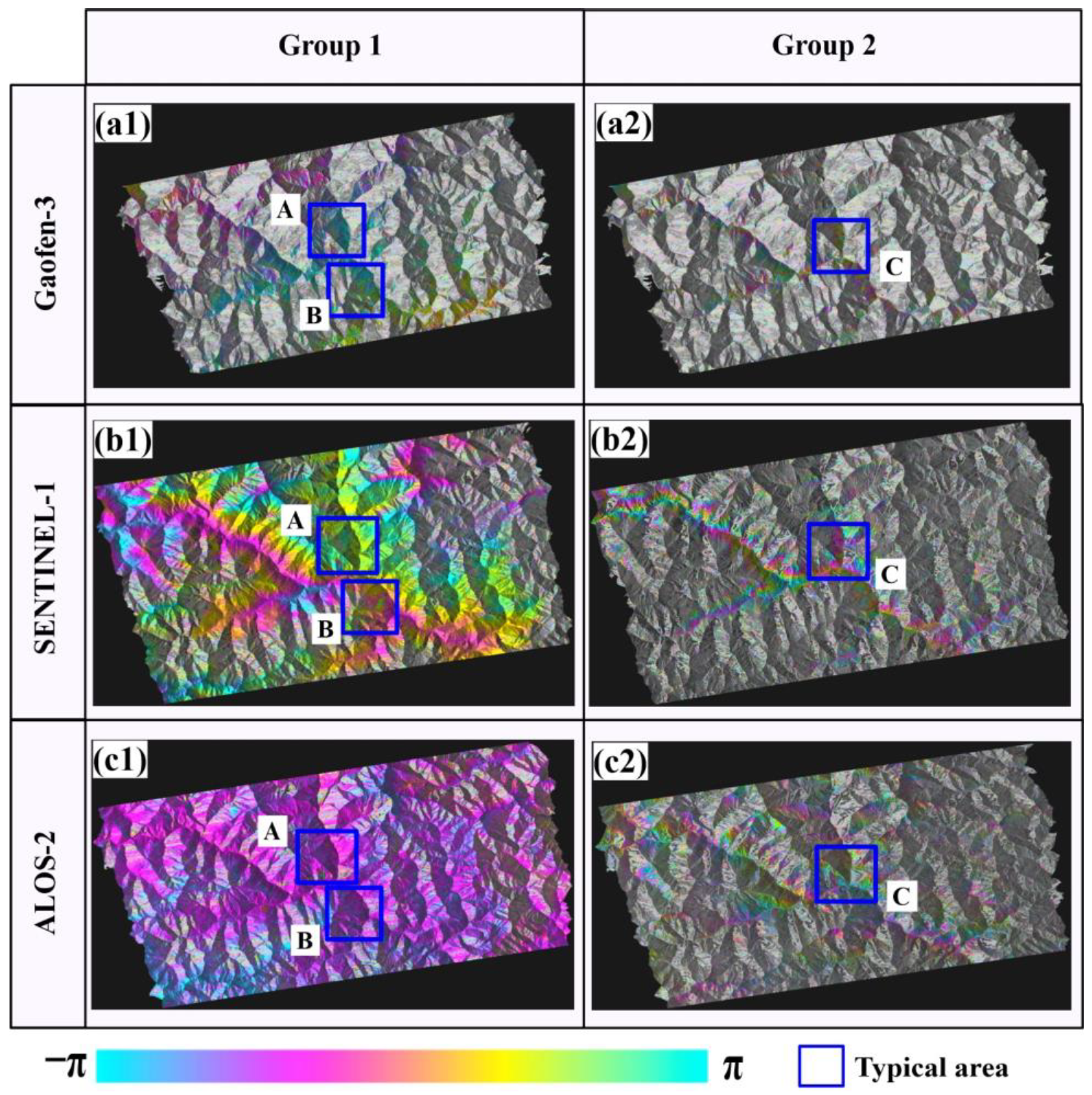
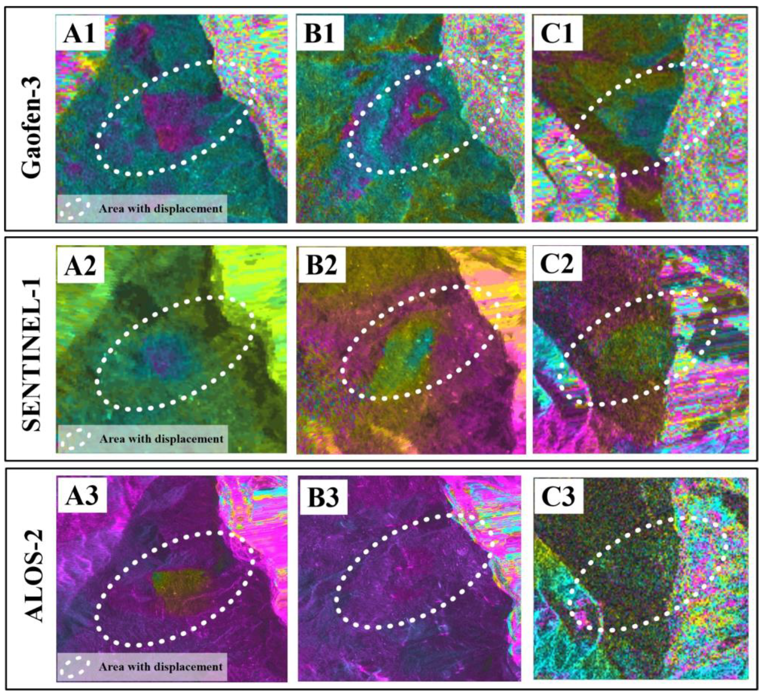
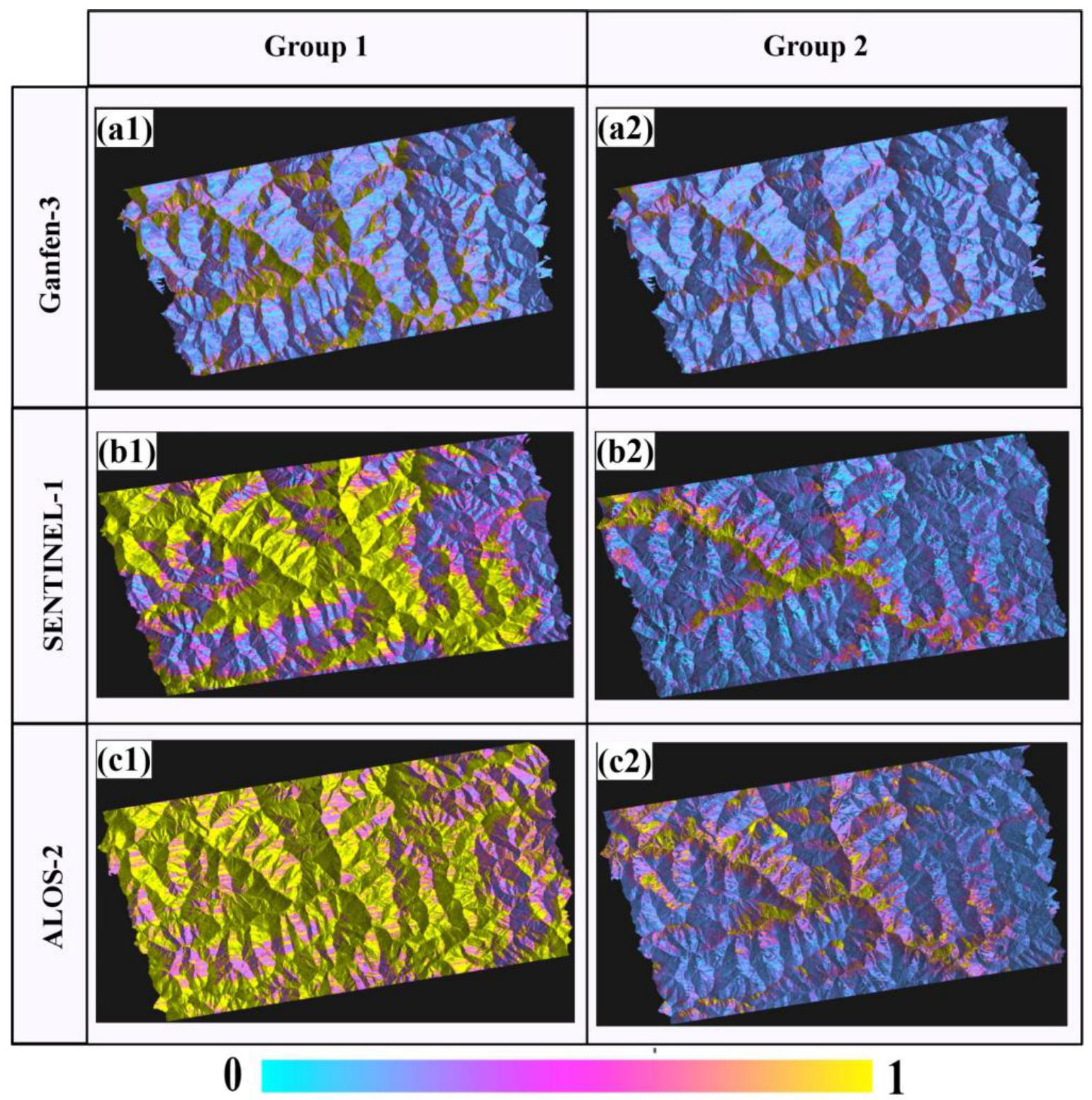
4.1. Analysis of the Interference Effect and Displacement Sensitivity
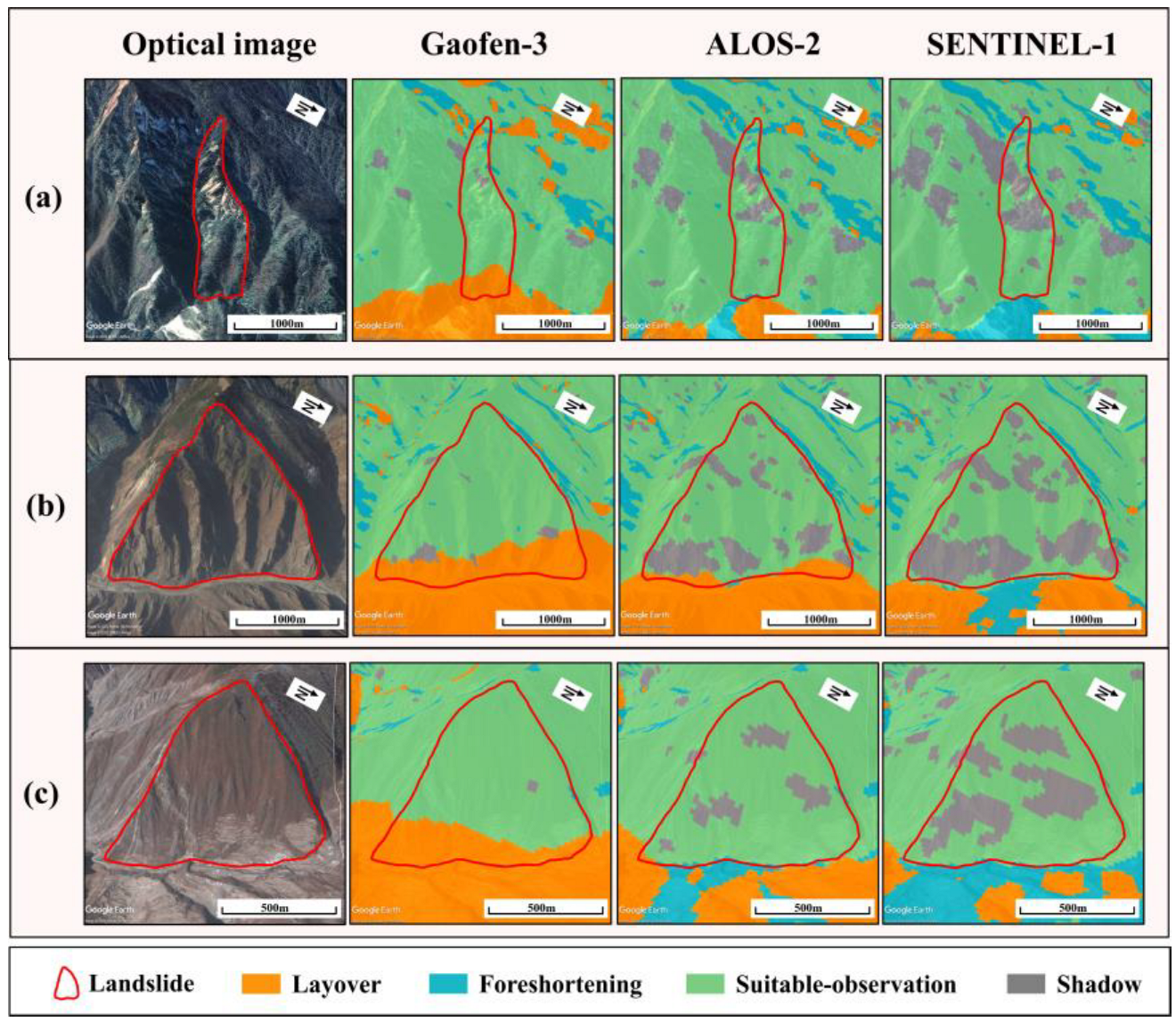
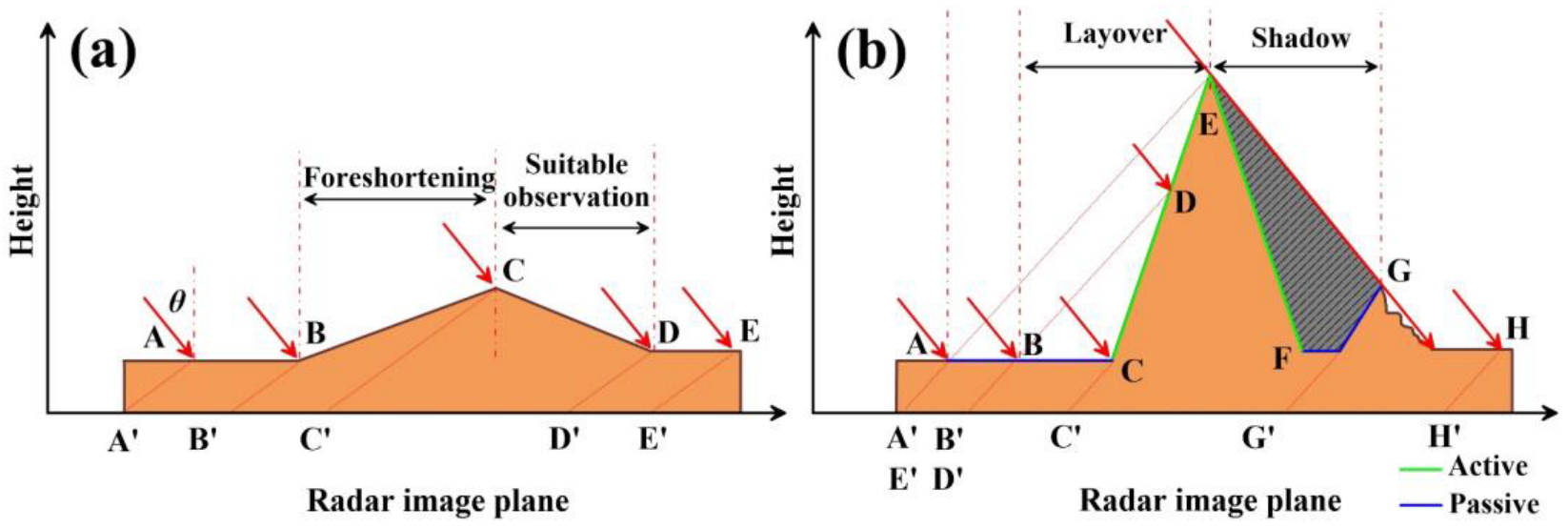
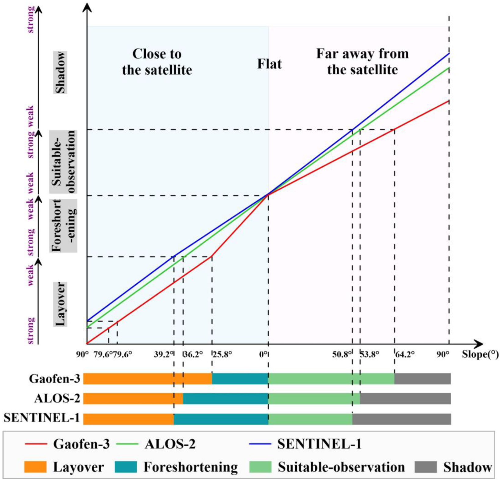
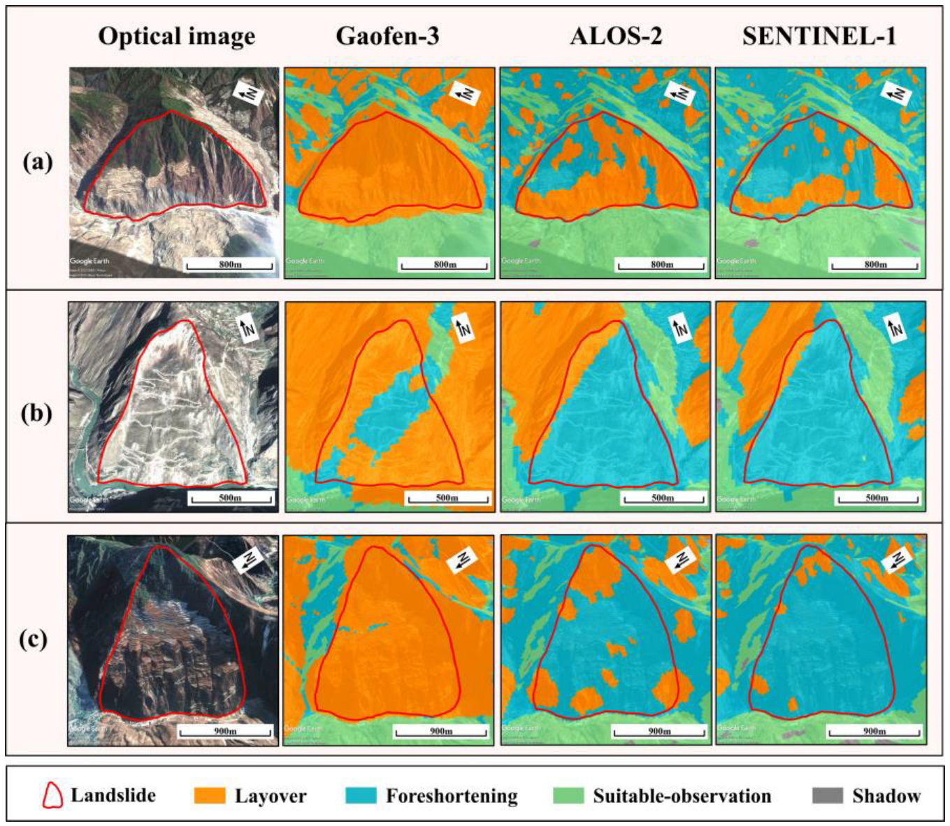
4.2. Observation Applicability Analysis of the SAR Data
5. Conclusions
Author Contributions
Funding
Data Availability Statement
Conflicts of Interest
References
- Dai, K.; Li, Z.; Xu, Q.; Bürgmann, R.; Milledge, D.G.; Tomas, R.; Fan, X.; Zhao, C.; Liu, X.; Peng, J.; et al. Entering the era of Earth-Observation based landslide warning system. IEEE Geosci. Remote Sens. Mag. 2022, 8, 136–153. [Google Scholar] [CrossRef]
- Shi, X.; Xu, Q.; Zhang, L.; Zhao, K.; Dong, J.; Jiang, H.; Liao, M. Surface displacements of the heifangtai terrace in northwest china measured by x and c-band insar observations. Eng. Geol. 2019, 259, 105181. [Google Scholar] [CrossRef]
- Journault, J.; Macciotta, R.; Hendry, M.; Charbonneau, F.; Huntley, D.; Bobrowsky, P. Measuring displacements of the thompson river valley landslides, south of ashcroft, bc, canada, using satellite insar. Landslides 2018, 15, 621–636. [Google Scholar] [CrossRef]
- Tomás, R.; Pagán, J.I.; Navarro, J.A.; Cano, M.; Pastor, J.L.; Riquelme, A.; Cuevas-González, M.; Crosetto, M.; Barra, A.; Monserrat, O. Semi-automatic identification and pre-screening of geological–geotechnical deformational processes using persistent scatterer interferometry datasets. Remote Sens. 2019, 11, 1675. [Google Scholar] [CrossRef]
- Dai, K.; Deng, J.; Xu, Q.; Li, Z.; Shi, X.; Wen, N.; Zhang, L.; Zhuo, G. Interpretation and sensitivity analysis of the LOS displacements from InSAR in landslide measurement. GIScience Remote Sens. 2022, 59, 1226–1242. [Google Scholar] [CrossRef]
- Pirasteh, S.; Li, J. Landslides investigations from geoinformatics perspective: Quality, challenges, and recommendations. Geomatics. Nat. Hazards Risk 2017, 8, 448–465. [Google Scholar] [CrossRef]
- An, M.; Sun, Q.; Hu, J.; Tang, Y.; Zhu, Z. Coastline detection with gaofen-3 sar images using an improved fcm method. Sensors 2018, 18, 1898. [Google Scholar] [CrossRef]
- National Space Administration. Launch of Gaofen-3 Satellite. Available online: http://www.sastind.gov.cn/n152/n6641041/index.html (accessed on 5 July 2022).
- Kang, W.; Xiang, Y.; Wang, F.; Wan, L.; You, H. Flood detection in gaofen-3 sar images via fully convolutional networks. Sensors 2018, 18, 2915. [Google Scholar] [CrossRef]
- Liu, W.; Yang, J.; Zhao, J.; Shi, H.; Yang, L. An unsupervised change detection method using time-series of polsar images from radarsat-2 and gaofen-3. Sensors 2018, 18, 559. [Google Scholar] [CrossRef] [PubMed]
- Zhang, L.; Xia, J. Flood detection using multiple chinese satellite datasets during 2020 china summer floods. Remote Sens. 2021, 14, 51. [Google Scholar] [CrossRef]
- Dong, H.; Xu, X.; Wang, L.; Pu, F. Gaofen-3 polsar image classification via xgboost and polarimetric spatial information. Sensors 2018, 18, 611. [Google Scholar] [CrossRef] [PubMed]
- Fang, Y.; Zhang, H.; Mao, Q.; Li, Z. Land cover classification with gf-3 polarimetric synthetic aperture radar data by random forest classifier and fast super-pixel segmentation. Sensors 2018, 18, 2014. [Google Scholar] [CrossRef] [PubMed]
- Chen, F. Comparing methods for segmenting supra-glacial lakes and surface features in the mount everest region of the himalayas using chinese gaofen-3 sar images. Remote Sens. 2021, 13, 2429. [Google Scholar] [CrossRef]
- Wang, Q.; Zhang, Y.; Fan, J.; Fu, Y. Monitoring the motion of the yiga glacier using gf-3 images. Geomat. Inf. Sci. Wuhan Univ. 2020, 45, 460–466. [Google Scholar]
- Wang, Y.; Wang, C.; Zhang, H.; Dong, Y.; Wei, S. Automatic ship detection based on retinanet using multi-resolution gaofen-3 imagery. Remote Sensing 2019, 11, 531. [Google Scholar] [CrossRef]
- An, Q.; Pan, Z.; You, H. Ship detection in gaofen-3 sar images based on sea clutter distribution analysis and deep convolutional neural network. Sensors 2018, 18, 334. [Google Scholar] [CrossRef]
- Zhang, L.; Meng, Q.; Zeng, J.; Wei, X.; Shi, H. Evaluation of gaofen-3 c-band sar for soil moisture retrieval using different polarimetric decomposition models. IEEE J. Sel. Top. Appl. Earth Obs. Remote Sens. 2021, 14, 5707–5719. [Google Scholar] [CrossRef]
- Zhang, L.; Meng, Q.; Yao, S.; Wang, Q.; Zeng, J.; Zhao, S.; Ma, J. Soil moisture retrieval from the chinese gf-3 satellite and optical data over agricultural fields. Sensors 2018, 18, 2675. [Google Scholar] [CrossRef]
- Han, L.; Wang, C.; Yu, T.; Gu, X.; Liu, Q. High-precision soil moisture mapping based on multi-model coupling and background knowledge, over vegetated areas using chinese gf-3 and gf-1 satellite data. Remote Sens. 2020, 12, 2123. [Google Scholar] [CrossRef]
- Li, N.; Guo, Z.; Zhao, J.; Wu, L.; Guo, Z. Characterizing ancient channel of the yellow river from spaceborne sar: Case study of chinese gaofen-3 satellite. IEEE Geosci. Remote Sens. Lett. 2021, 19, 1–5. [Google Scholar] [CrossRef]
- Ding, Y.; Liu, M.; Li, S.; Jia, D.; Zhou, L.; Wu, B.; Wang, Y. Mountainous landslide recognition based on gaofen-3 polarimetric sar imagery. In Proceedings of the IGARSS 2019–2019 IEEE International Geoscience and Remote Sensing Symposium, Yokohama, Japan, 28 July–2 August 2019; pp. 9634–9637. [Google Scholar]
- Jia, W.; Mengfei, W.; Jiang, D. Detecting recent landslide activities in yigong and surrounding areas in eastern tibet of china based on gf-3 sar amplitude imagery. In Proceedings of the IGARSS 2020-2020 IEEE International Geoscience and Remote Sensing Symposium, Waikoloa, HI, USA, 26 September–2 September 2020; pp. 5151–5154. [Google Scholar]
- Li, Q.; Zhang, J. Investigation on earthquake-induced landslide in jiuzhaigou using full polarimetric gf-3 sar images. J. Remote Sens. 2019, 23, 883–889l. [Google Scholar]
- China Earthquake Network Center. Earthquake. Available online: https://news.ceic.ac.cn/ (accessed on 5 July 2022).
- Intrieri, E.; Raspini, F.; Fumagalli, A.; Lu, P.; Del Conte, S.; Farina, P.; Allievi, J.; Ferretti, A.; Casagli, N. The Maoxian landslide as seen from space: Detecting precursors of failure with Sentinel-1 data. Landslides 2018, 15, 123–133. [Google Scholar]
- Sun, J.; Yu, W.; Deng, Y. The sar payload design and performance for the gf-3 mission. Sensors 2017, 17, 2419. [Google Scholar]
- Shang, M.; Han, B.; Ding, C.; Sun, J.; Zhang, T.; Huang, L.; Meng, D. A high-resolution sar focusing experiment based on gf-3 staring data. Sensors 2018, 18, 943. [Google Scholar] [CrossRef] [PubMed] [Green Version]
- Qingjun, Z. System design and key technologies of the gf-3 satellite. Acta Geod. Cartogr. Sin. 2017, 46, 269. [Google Scholar]
- Han, B.; Ding, C.; Zhong, L.; Liu, J.; Qiu, X.; Hu, Y.; Lei, B. The gf-3 sar data processor. Sensors 2018, 18, 835. [Google Scholar] [CrossRef]
- Zhang, Q.; Xiao, F.; Ding, Z.; Ke, M.; Zeng, T. Sliding spotlight mode imaging with gf-3 spaceborne sar sensor. Sensors 2017, 18, 43. [Google Scholar] [CrossRef]
- Potin, P.; Rosich, B.; Grimont, P.; Miranda, N.; Shurmer, I.; O’Connell, A.; Torres, R.; Krassenburg, M. Sentinel-1 mission status. In Proceedings of the EUSAR 2016: 11th European Conference on Synthetic Aperture Radar, Hamburg, Germany, 6–9 June 2016; pp. 1–6. [Google Scholar]
- Torres, R.; Snoeij, P.; Geudtner, D.; Bibby, D.; Davidson, M.; Attema, E.; Potin, P.; Rommen, B.; Floury, N.; Brown, M. Gmes sentinel-1 mission. Remote Sens. Environ. 2012, 120, 9–24. [Google Scholar]
- Arikawa, Y.; Saruwatari, H.; Hatooka, Y.; Suzuki, S. ALOS-2 launch and early orbit operation result. In Proceedings of the 2014 IEEE geoscience and remote sensing symposium, Quebec City, QC, Canada, 13–18 July 2014; pp. 3406–3409. [Google Scholar]
- Xu, X.; Ma, C.; Shan, X.; Lian, D.; Qu, C.; Bai, J. Monitoring Ground Subsidence in High-intensity Mining Area by lntegrating DInSAR and Offset-tracking Technology. J. Geo-Inf. Sci. 2020, 22, 2425–2435. [Google Scholar]
- Mao, W.; Liu, G.; Wang, X.; Xie, Y.; He, X.; Zhang, B.; Xiang, W.; Wu, S.; Zhang, R.; Fu, Y. Using Range Split-Spectrum Interferometry to Reduce Phase Unwrapping Errors for InSAR-Derived DEM in Large Gradient Region. Remote Sens. 2022, 14, 2607. [Google Scholar] [CrossRef]
- Suganthi, S.; Elango, L.; Subramanian, S. Microwave d-insar technique for assessment of land subsidence in kolkata city, india. Arab. J. Geosci. 2017, 10, 458. [Google Scholar] [CrossRef]
- Poreh, D.; Pirasteh, S. InSAR and Landsat ETM+ incorporating with CGPS and SVM to determine subsidence rates and effects on Mexico City. Geoenvironmental Disasters 2019, 8, 2–19. [Google Scholar] [CrossRef]
- Zhao, L.; Liang, R.; Shi, X.; Dai, K.; Cheng, J.; Cao, J. Detecting and analyzing the displacement of a small-magnitude earthquake cluster in rong county, china by the gacos based insar technology. Remote Sens. 2021, 13, 4137. [Google Scholar] [CrossRef]
- Li, W.; Zhou, Y. Early warning and monitoring of geohazards based on D-InSAR technology. Eng. Surv. Mapp. 2021, 30, 66–70. [Google Scholar]
- Dai, K.; Li, Z.; Tomás, R.; Liu, G.; Yu, B.; Wang, X.; Cheng, H.; Chen, J.; Stockamp, J. Monitoring activity at the daguangbao mega-landslide (China) using sentinel-1 tops time series interferometry. Remote Sens. Environ. 2016, 186, 501–513. [Google Scholar] [CrossRef]
- Dai, K.; Zhang, L.; Song, C.; Li, Z.; Zhuo, G.; Xu, Q. Quantitative Analysis of Sentinel-1 lmagery Geometric Distortion and Their Suitability Along Sichuan-Tibet Railway. Geomat. Inf. Sci. Wuhan Univ. 2021, 46, 1450–1460. [Google Scholar]
- Shi, X.; Dai, K.; Deng, J.; Zhong, D.; Liu, G.; Pirasteh, S.; Zhang, B.; Ali, Y.P.; He, Y.; Liang, R. Spatio-temporal evolutionary characteristics of gongga mountain glaciers and their response to climate. Adv. Space Res. 2021, 68, 1706–1718. [Google Scholar] [CrossRef]


| Gaofen-3 | ALOS-2 | SENTINEL-1 |
|---|---|---|
| 8 March 2020 | 26 November 2017 | 29 December 2020 |
| 8 June 2020 | 24 December 2017 | 10 January 2021 |
| 3 September 2020 | 4 February 2018 | 22 January 2021 |
| 31 October 2020 | 15 April 2018 | 3 February 2021 |
| 28 December 2020 | 13 May 2018 | 15 February 2021 |
| 26 January 2021 | 10 June 2018 | 27 February 2021 |
| 24 February 2021 | 8 July 2018 | 11 March 2021 |
| 25 March 2021 | 5 August 2018 | 23 March 2021 |
| 23 April 2021 | 2 September 2018 | 4 April 2021 |
| 14 October 2018 | 16 April 2021 | |
| 31 March 2019 | 28 April 2021 |
| Parameters | Gaofen-3 | ALOS-2 | SENTINEL-1 |
|---|---|---|---|
| Orbital track | Ascending | Ascending | Ascending |
| Imaging mode | FS1 | UBS | IW |
| Range pixel spacing (m) | 1.12 | 1.43 | 2.33 |
| Azimuth pixel spacing (m) | 2.59 | 2.13 | 13.92 |
| Polarization | HH | HH | VV |
| Incidence angle (°) | 25.8 | 36.2 | 39.2 |
| Interference Pair | Time Baseline (d) | Spatial Baseline (m) |
|---|---|---|
| 3 September 2020–31 October 2020 | 58 | 1608 |
| 3 September 2020–28 December 2020 | 116 | 868 |
| 3 September 2020–26 January 2021 | 145 | 1120 |
| 3 September 2020–24 February 2021 | 174 | −131 |
| 3 September 2020–25 March 2021 | 203 | 306 |
| 31 October 2020–26 January 2021 | 87 | −487 |
| 31 October 2020–24 February 2021 | 116 | −1627 |
| 31 October 2020–25 March 2021 | 145 | −1312 |
| 31 October 2020–23 April 2021 | 174 | −215 |
| 28 December 2020–26 January 2021 | 29 | 265 |
| 28 December 2020–24 February 2021 | 58 | −900 |
| 28 December 2020–25 March 2021 | 87 | −582 |
| 28 December 2020–23 April 2021 | 116 | 556 |
| 26 January 2021–24 February 2021 | 29 | −1142 |
| 26 January 2021–25 March 2021 | 58 | −825 |
| 26 January 2021–23 April 2021 | 87 | 313 |
| 24 February 2021–25 March 2021 | 29 | 318 |
| 24 February 2021–23 April 2021 | 58 | 1450 |
| 25 March 2021–23 April 2021 | 29 | 1132 |
| Data Source | Gaofen-3 | SENTINEL-1 | ALOS-2 | |
|---|---|---|---|---|
| Group 1 | Time | 28 December 2020–26 January 2021 | 29 December 2020–3 February 2021 | 24 December 2017–4 February 2018 |
| Time Baseline (d) | 29 | 36 | 42 | |
| Spatial Baseline (m) | 265 | 87 | −215 | |
| Group 2 | Time | 26 January 2021–23 April 2021 | 22 January 2021–16 April 2021 | 4 February 2018–13 May 2018 |
| Time Baseline (d) | 87 | 84 | 98 | |
| Spatial Baseline (m) | 313 | −93 | 201 |
| Observation Information | Gaofen-3 | ALOS-2 | SENTINEL-1 |
|---|---|---|---|
| Layover | 51.3% | 27.7% | 17.9% |
| Foreshortening | 8.9% | 23.7% | 28.8% |
| Shadow | 0.2% | 1.9% | 5.8% |
| Theoretical suitable observation | 71.3% | 59.8% | 56.4% |
| Actual suitable observation | 39.6% | 46.7% | 47.5% |
Publisher’s Note: MDPI stays neutral with regard to jurisdictional claims in published maps and institutional affiliations. |
© 2022 by the authors. Licensee MDPI, Basel, Switzerland. This article is an open access article distributed under the terms and conditions of the Creative Commons Attribution (CC BY) license (https://creativecommons.org/licenses/by/4.0/).
Share and Cite
Wen, N.; Zeng, F.; Dai, K.; Li, T.; Zhang, X.; Pirasteh, S.; Liu, C.; Xu, Q. Evaluating and Analyzing the Potential of the Gaofen-3 SAR Satellite for Landslide Monitoring. Remote Sens. 2022, 14, 4425. https://doi.org/10.3390/rs14174425
Wen N, Zeng F, Dai K, Li T, Zhang X, Pirasteh S, Liu C, Xu Q. Evaluating and Analyzing the Potential of the Gaofen-3 SAR Satellite for Landslide Monitoring. Remote Sensing. 2022; 14(17):4425. https://doi.org/10.3390/rs14174425
Chicago/Turabian StyleWen, Ningling, Fanru Zeng, Keren Dai, Tao Li, Xi Zhang, Saied Pirasteh, Chen Liu, and Qiang Xu. 2022. "Evaluating and Analyzing the Potential of the Gaofen-3 SAR Satellite for Landslide Monitoring" Remote Sensing 14, no. 17: 4425. https://doi.org/10.3390/rs14174425
APA StyleWen, N., Zeng, F., Dai, K., Li, T., Zhang, X., Pirasteh, S., Liu, C., & Xu, Q. (2022). Evaluating and Analyzing the Potential of the Gaofen-3 SAR Satellite for Landslide Monitoring. Remote Sensing, 14(17), 4425. https://doi.org/10.3390/rs14174425