Calculating Co-Seismic Three-Dimensional Displacements from InSAR Observations with the Dislocation Model-Based Displacement Direction Constraint: Application to the 23 July 2020 Mw6.3 Nima Earthquake, China

Abstract

As one of the most prevailing geodetic tools, the interferometric synthetic aperture radar (InSAR) technique can accurately obtain co-seismic displacements, but is limited to the one-dimensional line-of-sight (LOS) measurement. It is therefore difficult to completely reveal the real three-dimensional (3D) surface displacements with InSAR. By employing azimuth displacement observations from pixel offset tracking (POT) and multiple aperture InSAR (MAI) techniques, 3D displacements of large-magnitude earthquakes can be obtained by integrating the ascending and descending data. However, this method cannot be used to accurately realize the 3D surface displacement measurements of small-magnitude earthquakes due to the low accuracies of the POT/MAI-derived azimuth displacement measurements. In this paper, an alternative method is proposed to calculate co-seismic 3D displacements from ascending and descending InSAR-LOS observations with the dislocation model-based displacement direction constraint. The main contribution lies in the two virtual observation equations that are obtained from the dislocation model-based forward-modeling 3D displacements, which are then combined with the ascending/descending InSAR observations to calculate the 3D displacements. The basis of the two virtual observation equations is that the directions of the 3D displacement vectors are very similar for real and model-based 3D displacements. In addition, the weighted least squares (WLS) method is employed to solve the final 3D displacements, which aims to consider and balance the possible errors in the InSAR observations as well as the dislocation model-based displacement direction constraint. A simulation experiment demonstrates that the proposed method can achieve more accurate 3D displacements compared with the existing methods. The co-seismic 3D displacements of the 2020 Nima earthquake are then accurately obtained by the proposed method. The results show that co-seismic displacements are dominated by the vertical displacement, the magnitude of the horizontal displacement is relatively small, and the overall displacement pattern fits well with the tensile rupture.

1. Introduction

Complete and accurate co-seismic three-dimensional (3D) displacements can provide intuitive data for seismic interpretation and hazard assessment. The global navigation satellite system (GNSS) and interferometric synthetic aperture radar (InSAR) are the most widely used observation tools for constructing the surface displacement recordings. However, it is difficult to obtain sufficient GNSS data for ground motions caused by sudden strong earthquakes occurring in remote areas. In recent years, Synthetic Aperture Radar (SAR) data-based techniques for measuring surface displacements have been well developed, including the differential interferometric SAR (InSAR, DInSAR) [1], pixel offset tracking (POT) [2], multiple aperture InSAR (MAI) [3], and burst overlap InSAR (BOI) [4] methods, providing sufficient displacement observations for measuring co-seismic 3D displacements. Although it is feasible to obtain co-seismic 3D displacements by combining DInSAR-derived line-of-sight (LOS) observations and POT/MAI/BOI-derived azimuth observations from ascending and descending SAR data [5,6,7,8], these kinds of methods are not suitable to calculate 3D displacements for small-magnitude earthquakes since the accuracy of POT/MAI/BOI observations is too low to derive reliable azimuth displacements [3,9,10].

In recent years, several researchers proposed to estimate complete co-seismic 3D displacement measurements by incorporating additional a priori information based on the fault dislocation model [11,12,13,14]. For example, Song et al. [12] generated the initial 3D displacements field based on a small number of GNSS data and the elastic dislocation model, then combined these with InSAR observations to obtain the final 3D displacements of the Wenchuan earthquake based on the robust weighting methods (e.g., the Best Quadratic Unbiased Estimator, BQUE). Similarly, Qu et al. [11] firstly obtained the north–south displacement component by the dislocation forward modeling, then calculated the east–west and vertical components based on the known north–south component and ascending/descending InSAR observations. Recently, Xu et al. [14] demonstrated from a series of experiments that the directions of dislocation forward modeling co-seismic 3D displacement vectors would change very little for different dislocation model parameters in the inversion process. In this sense, the vector direction of the forward modeling co-seismic 3D displacements is used as a constraint to estimate the 3D displacements of the 2008 Wenchuan earthquake based on a single-track InSAR-LOS displacement. Although it is demonstrated that the 3D displacements can be solved by using the displacement vector direction as a constraint [13,14], this method solves the 3D displacements directly through a displacement direction constraint, without considering the effect of observation error. At the same time, the displacement vector direction based on the forward-modeling 3D displacements will inevitably contain errors with respect to the real 3D displacements, therefore degrading the reliability of the final co-seismic 3D displacements.

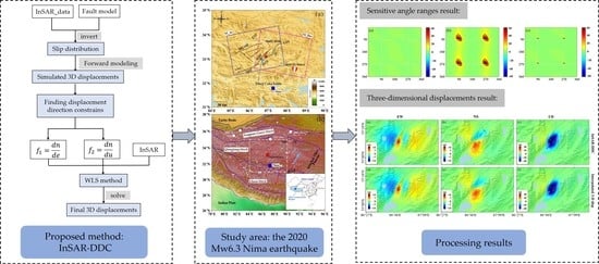
Hence, this paper proposes an alternative method that calculates co-seismic 3D displacements from ascending and descending InSAR observations with the dislocation model-based displacement direction constraint. The proposed method relies on the establishment of two virtual observation equations, which represent the a priori information about the 3D displacement directions based on the dislocation forward-modeling 3D displacements. Then, these two virtual observation equations are combined with the ascending/descending InSAR observations to calculate the co-seismic 3D displacements. Considering that the InSAR observation as well as the direction constraint are both vulnerable to the errors, the weighted least squares (WLS) method is employed to obtain the final co-seismic 3D displacements. Simulation experiments are firstly conducted to validate the proposed method in this paper, and the high-precision co-seismic 3D displacements of the 2020 Nima earthquake are then successfully obtained. The 2020 Mw6.3 Nima earthquake occurred in Nima County, Tibet Autonomous Region, China, with the seismogenic fault being the West Yibug Caka fault (WYF). This earthquake exhibited complex fault kinematic features and significant surface displacements. It is therefore of great significance to map complete 3D displacements for interpreting this seismic event.

2. Study Area

At 04:07:20 a.m. on 23 July 2020 (local time), an Mw6.3 earthquake attacked Nima County, Tibet Autonomous Region, China. This earthquake was located on the Tibetan Plateau, which is one of the regions with the strongest tectonic and seismic activities in China [15]. Around the Tibetan Plateau, these seismic events occur frequently and most of them are shallow earthquakes due to the long-term extrusion and collision between the Indian and Eurasian plates. The Lhasa and Qiangtang blocks are located in the center of the Tibetan Plateau, and their collisional connection is Bangong–Nujiang suture (BNS) zone, where a series of conjugate strike-slip faults and near NS-trending grabens have developed. 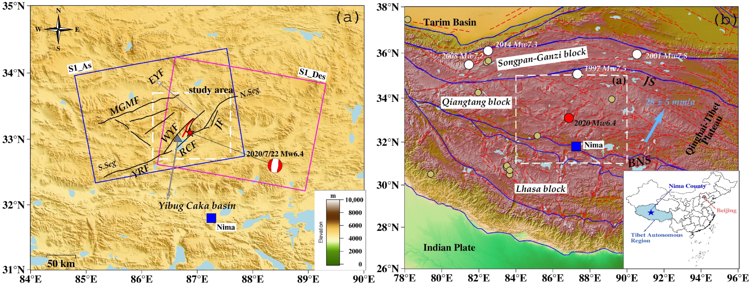Since 1997, a dozen earthquakes of magnitude 6 or higher have occurred around this area (Figure 1), including four destructive earthquakes of magnitude 7 or greater (i.e., the 1997 Mani Mw7.5 earthquake in Tibet, the 2001 Mw7.8 earthquake in southern Qinghai, the 2008 Yutian Mw7.2 earthquake in Xinjiang, and the 2014 Yutian Mw7.3 earthquake in Xinjiang).

The 2020 Mw6.3 Nima earthquake occurred in the core zone of the central uplift of the Qiangtang block, with extremely complex regional tectonics [16]. The Qiangtang block, dominated by NE60° motion with an average velocity of 28 ± 5 mm/a, is located between two major fault zones, i.e., the BNS and the Jinsha River suture (JS) zones, and the active tectonics are more developed in this region [17]. The main active fault system crossing the epicenter of the 2020 Nima earthquake is the Riganpei Co–Yibu Chaka–Jiangai Zangbu fault (RYJF), which shows a NE-striking and belongs to the northern branch of the Dong Co conjugate fault system. The RYJF consists of three fault segments, of which the northern and southern segments are left-lateral strike-slips, and the central segment is dominated by the normal-faulting mechanism [18,19]. The epicenter of the 2020 Nima earthquake was located approximately 4 km east of the northern end of the West Yibug Caka fault (WYF) in the central part of the RYJF [20]. The proximity of the epicenter to the WYF indicates that the fault on which this earthquake occurred is related to the active WYF.

3. Methods

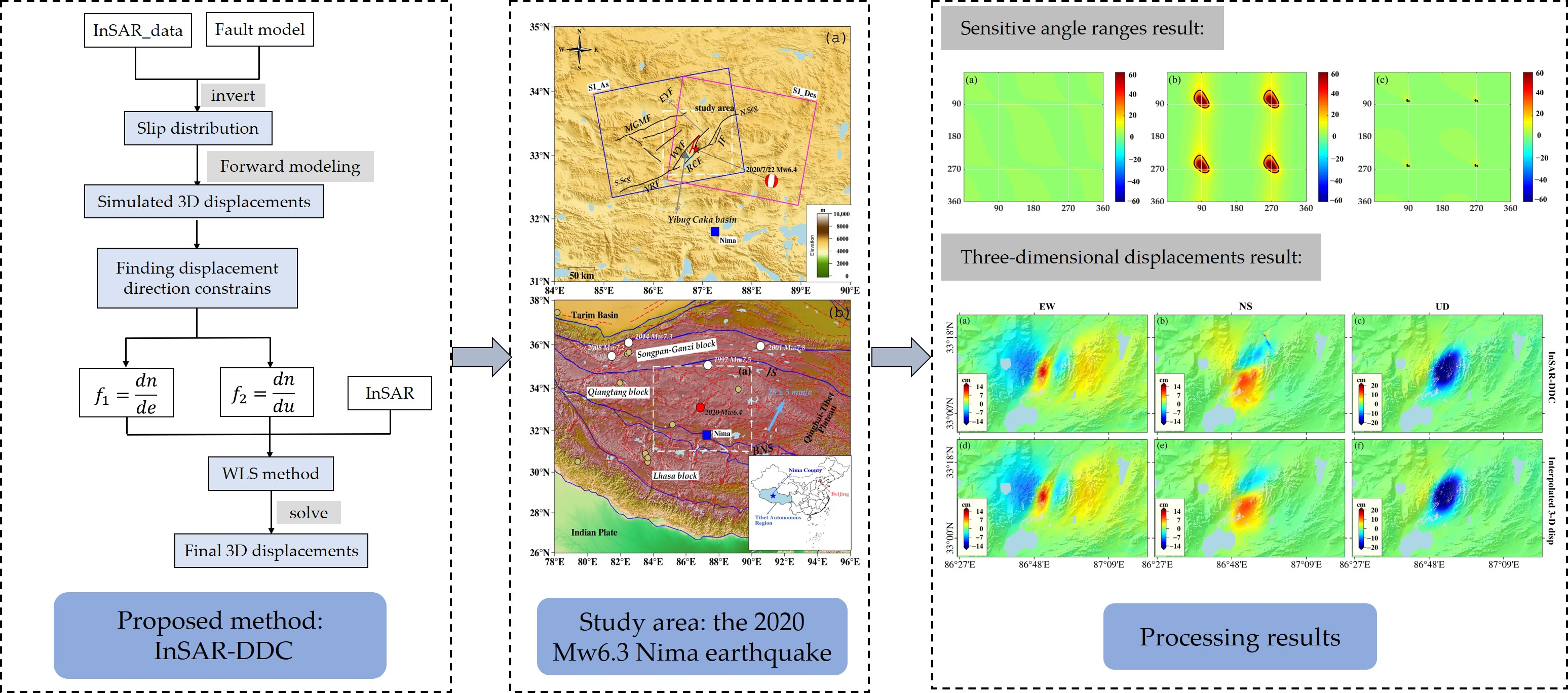
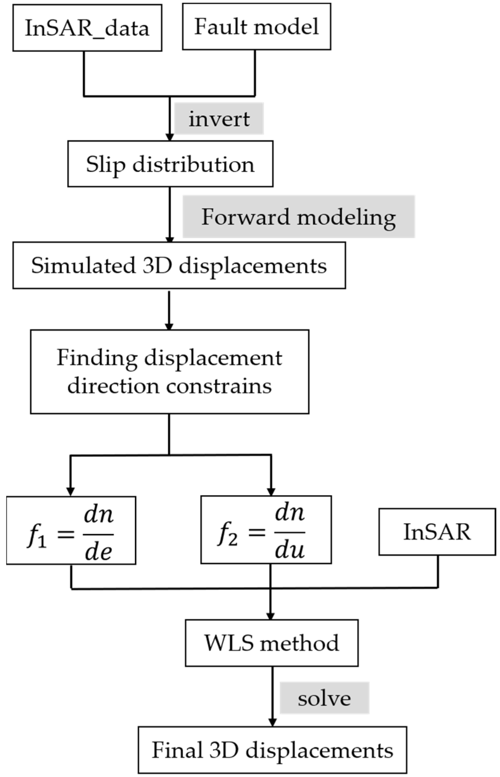
For small-magnitude earthquakes, given that only the two ascending and descending DInSAR displacement observations can be obtained to completely cover the whole study area, it is almost impractical to directly obtain the accurate co-seismic 3D displacements based only on these two observations. Therefore, this paper proposes a method to calculate co-seismic 3D displacements from InSAR observations with the dislocation model-based displacement direction constraint (here referred to as InSAR-DDC method). After obtaining ascending and descending data, the 3D displacements can be solved by this new method. The main steps include the following:

(1)

Based on the fault dislocation model and InSAR observations, we can obtain simulated co-seismic 3D displacements by inversion and forward modeling.

(2)

Based on the simulated co-seismic 3D displacements, two vectors consisting of north–south and east–west components, and north–south and vertical components are formed, respectively, and the directions of these two vectors are used as a priori information to establish two virtual observation equations.

(3)

By combining the InSAR observations and two virtual observation equations, the WLS method is used to calculate the final co-seismic 3D displacements.

The specific implementation process of the proposed method is described in detail in the following, and the flowchart is shown in Figure 2.

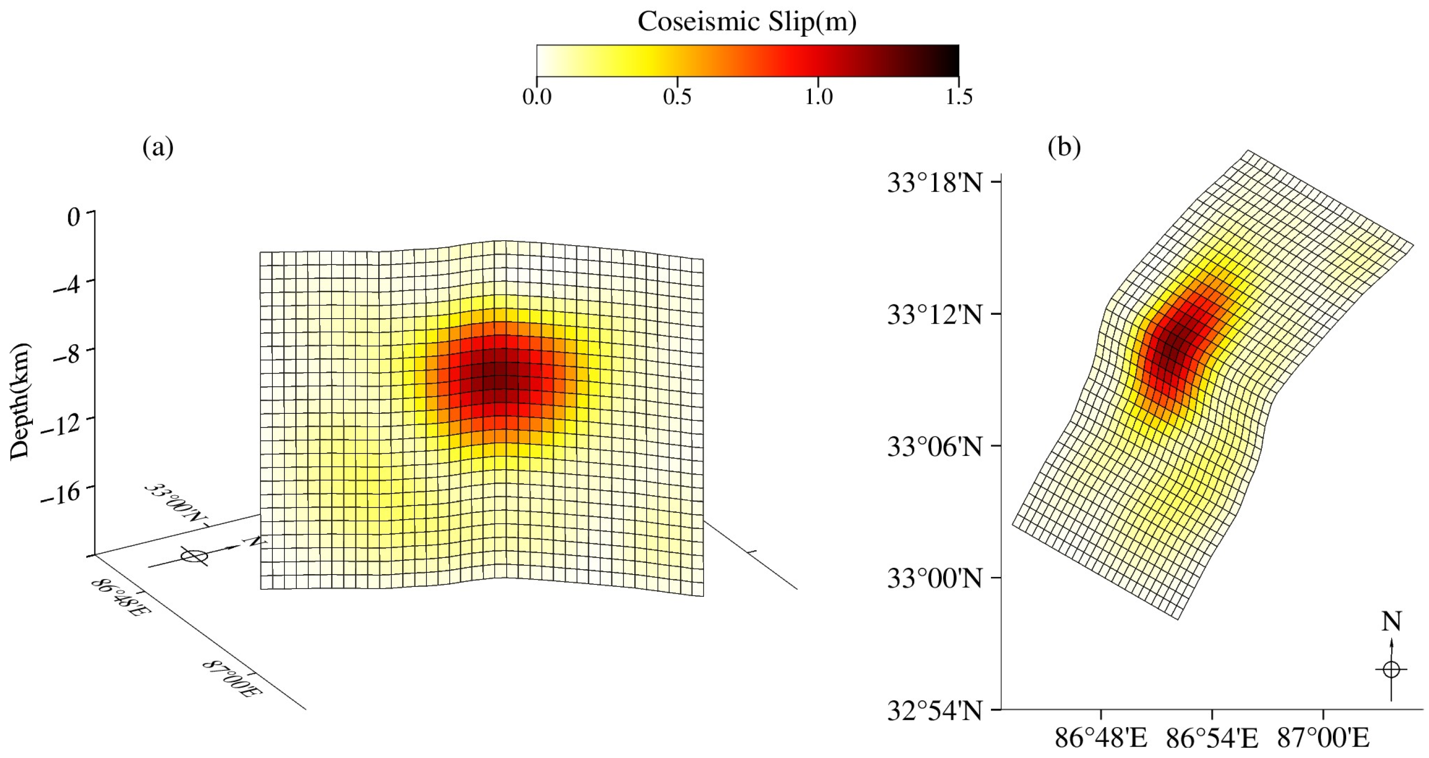
3.1. Simulating Co-Seismic 3D Displacements Based on the Fault Dislocation Model

Before obtaining co-seismic 3D displacement simulations from the dislocation model, it is necessary to derive the fault slip distribution of earthquakes. The relationship between the InSAR observations and the fault slip distribution is [21]

$$\left[\begin{array}{c}G\\ {\alpha }^{2}H\end{array}\right]S=\left[\begin{array}{c}{d}_{LOS}\\ 0\end{array}\right]$$

(1)

where $H$ is the second-order finite-difference operator for estimating the roughness of the slip, $\alpha$ is the smoothing factor to balance the trade-off between the data misfit and the slip roughness [22],$G$ is the Green’s function, $d_{LOS}$ is the InSAR observation, and $\mathit{S}$ is the total slip of m discrete patches in the fault plane.

Before calculating the slip on the fault plane, we need to divide the whole fault plane into $m$ discrete patches, which are independent of each other and may cause the problem of discontinuous slip values. Therefore, a priori information and artificial constraints are needed to ensure that the slip distribution is smooth and physically reasonable. A common approach among various inversion methods is to add a penalty term to the misfit function to minimize the roughness of the slip distribution, as the second-order finite-difference operator $H$ in Equation (1).

After the inversion of the slip distribution, the co-seismic 3D displacements can be obtained by forward modeling based on the fault dislocation model. The linear response relationship between fault slip at a certain depth underground and the surface displacements is shown in Equation (2)

$$S_{E/N/U}={\displaystyle \sum }_{j=1}^m\left(G_{ij}^x{S}_j^x+G_{ij}^y{S}_j^y\right)$$

(2)

where $S_j^x,S_j^y\left(j=1,2....m\right)$ are the strike and dip slip of the jth discrete patch in the fault plane, respectively, $S_E,S_N,S_U$ are the forward-modeling simulated east–west, north–south, and vertical displacements, respectively. Due to the uncertainty and non-uniqueness of the model parameters in the inversion, the accuracy of the simulated 3D displacements obtained from the forward modeling cannot be well guaranteed. The following two steps (i.e., Section 3.2 and Section 3.3) of the proposed method should be conducted to obtain more accurate co-seismic 3D displacements.

3.2. Constructing Two Virtual Observation Equations Based on Simulated Co-Seismic 3D Displacements

For a target point, the relationship between the InSAR-LOS observation $d_{LOS}$ and the 3D displacements $d_e,d_n,d_u$ can be expressed as [23]

$$d_{LOS}=-\mathit{sin}\theta \mathit{cos}\phi \cdot d_e+\mathit{sin}\theta \mathit{sin}\phi \cdot d_n+\mathit{cos}\theta \cdot d_u$$

(3)

where $\phi$ and $\theta$ are the satellite heading angle (clockwise from the north) and the radar incidence angle, respectively. $d_e,d_n,d_u$ are the final east–west, north–south, and vertical displacements, respectively. It is easy to infer from Equation (3) that the 3D displacements cannot be solved by using only two InSAR observations from ascending and descending tracks. In this sense, one of the focuses of the proposed method is how to incorporate the prior information provided by the fault dislocation model to constrain the 3D displacements, thus increasing the number of observation equations and making the 3D displacements solvable.

Xu et al. [14] obtained the simulated 3D displacements $d_N,d_E,d_U$ based on the forward modeling (i.e., Equation (2)), then under the experimental result where the directions of the real and simulated 3D displacements are very similar, the direction of simulated 3D displacement vector is used as a constraint to calculate the co-seismic 3D displacements of the 2008 Wenchuan earthquake by using only one InSAR-LOS observation. However, since no redundant observation is available, this method is highly susceptible to observation errors. In this paper, given the previous conclusion that the simulated 3D displacement directions are very similar to the real ones, we further obtain the following conditions: (i) The direction for the two-dimensional (2D) vector of north–south and east–west displacements is very similar for the simulated and real displacements. (ii) The direction for the 2D vector of north–south and vertical displacements is very similar for the simulated and real displacements. Here, the direction for the 2D vector of east–west and vertical displacements is not considered due to the fact that this vector direction can be deduced from (i) and (ii). Based on the simulated 3D displacements, the corresponding vector directions can be easily calculated, then be used as the a priori constraints to obtain the final co-seismic 3D displacements by combining with the ascending and descending InSAR observations. Assuming the vector directions in (i) and (ii) are angles $\alpha$ and $\beta$, respectively, the following equations can be obtained

$$\{\begin{array}{c}\frac{d_N}{d_E}=\mathit{tan}\alpha =f_1\\ \frac{d_N}{d_U}=\mathit{tan}\beta =f_2\end{array}$$

(4)

where $f_1$ and $f_2$ are the $tan$ value of angles $\alpha$ and $\beta$, respectively. Based on Equation (4), the corresponding virtual observation equations can be obtained as

$$\left[\begin{array}{c}0\\ 0\end{array}\right]=\left[\begin{array}{ccc}{f}_1& -1& 0\\ 0& -1& f_2\end{array}\right]\left[\begin{array}{c}{d}_e\\ d_n\\ d_u\end{array}\right]$$

(5)

Then, the following equation can be obtained by combining Equations (3) and (5)

$$B\cdot d=L$$

(6)

where $B$ is coefficient matrix, $L$ is observation vector, $d$ is unknown vector that includes the final 3D displacements. $B,d,L$ are expressed as follows

$$B=\left[\begin{array}{ccc}-\mathit{sin}{\theta }_1\mathit{cos}{\phi }_1& \mathit{sin}{\theta }_1\mathit{sin}{\phi }_1& \mathit{cos}{\theta }_1\\ -\mathit{sin}{\theta }_2\mathit{cos}{\phi }_2& \mathit{sin}{\theta }_2\mathit{sin}{\phi }_2& \mathit{cos}{\theta }_2\\ f_1& -1& 0\\ 0& -1& f_2\end{array}\right]$$

(7)

$$d={\left[\begin{array}{ccc}{d}_e& d_n& d_u\end{array}\right]}^T$$

(8)

$$L={\left[\begin{array}{cccc}{d}_{los1}& d_{los2}& 0& 0\end{array}\right]}^T$$

(9)

3.3. Calculating Co-Seismic 3D Displacements Based on the Weighted Least Squares

The complete 3D displacements can be directly calculated based on Equation (6) and the weighted least squares (WLS) method [24,25,26,27]. Generally, the level of observation errors can be represented by the variance matrix, and the weighting matrix $P_L$ is employed during the calculation process

$$P_L=diag\left(P_{los1},P_{los2},P_1,P_2\right)$$

(10)

where $P_{los1},P_{los2},P_1,P_2$ are the weights of four observations in $L$. If the real variance of each observation can be obtained, the weights $P_L$ can be easily determined. However, it is impractical to accurately determine the variance of each observation, making it hard to obtain the weights $P_L$.

Here, in order to determine the optimal values of different observations’ weights, a series of simulation experiments are conducted. Firstly, in the real experiment, the slip distribution of the earthquake is obtained by inversion of InSAR data and fault dislocation model, and then forward modeling is used to obtain simulated co-seismic 3D displacements. The simulated co-seismic 3D displacements in the real experiment are used as the true value of 3D displacements in the simulation experiments. To obtain the ascending/descending InSAR observations, the InSAR-LOS displacement signals are obtained based on the simulated 3D displacements, and the atmospheric noise signals are simulated by the fractal function based on the atmospheric noise level of the real data. Here, the real atmospheric noise level can be extracted during the fault inversion process. Based on the above steps, the simulated InSAR observations are obtained. Then, based on the simulated InSAR observations, the simulated co-seismic 3D displacements can be obtained based on the fault dislocation model. Afterwards, two virtual observation equations and two InSAR-LOS observations are combined to calculate the final 3D displacements (InSAR-DDC method). Here, the WLS method is used to solve the unknown parameters. Before solving the 3D displacements, it is necessary to determine the weight of the four observation values. In order to determine the optimal weights of these four observations, different values of $P_{los2},P_1,P_2$ are tested, where $P_{los1}$ is taken as the constant value of 1, and $P_{los2},P_1,P_2$ range from 0.01 to 1000. With traversaling of different values of $P_{los2},P_1,P_2$, the final 3D displacements can be calculated with the WLS method, and the corresponding RMSEs of 3D displacements can also be estimated. Here, the group of weights with the smallest RMSEs of 3D displacements is taken as the optimal value of $P_{los2},P_1,P_2$, which is also used to weight observations in the real experiment. Based on this process, the weights $P_{los1},P_{los2},P_1,P_2$ used in this paper are 1, 0.3162, 1, 0.1, respectively.

Based on the WLS method, the final 3D displacements can be calculated without calculation problems. The calculation equations are as follows

$$d={(B^T{P}_{L}B)}^{-1}{B}^T{P}_{L}L$$

(11)

4. Simulation Experiments

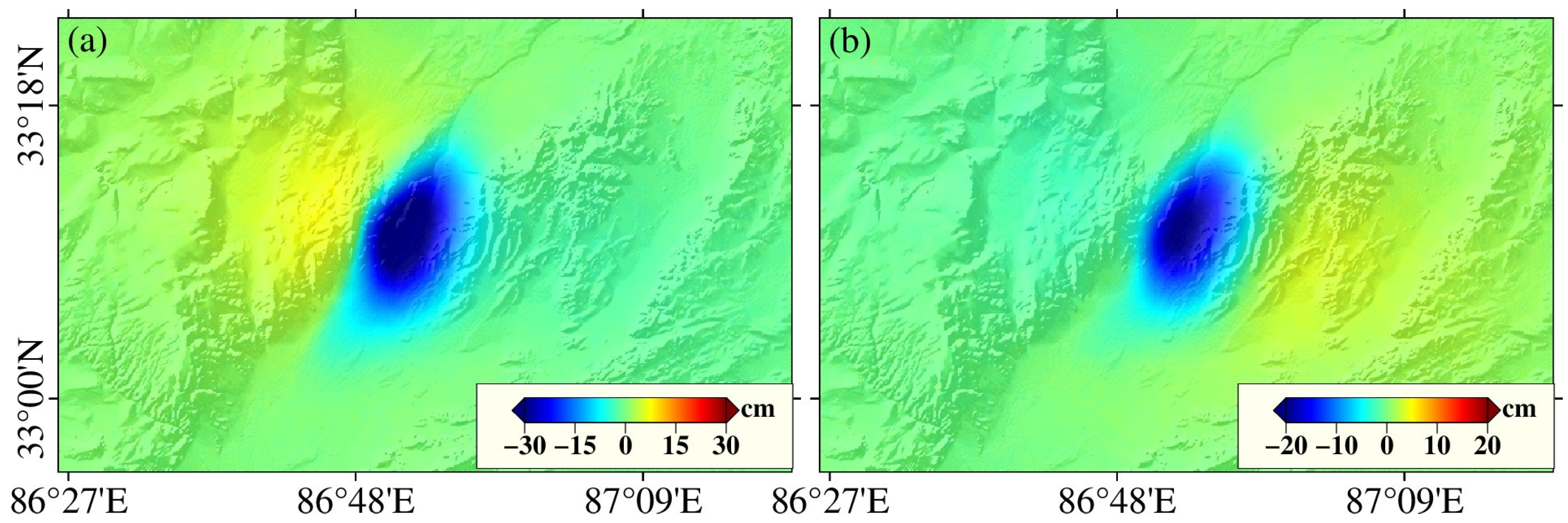
Simulation experiments are first conducted to verify the performance of the proposed method. The simulated co-seismic 3D displacements based on the fault dislocation model in the real experiments are used as the true value of 3D displacements in the simulations. As shown in Figure 3, the InSAR-LOS displacement signals are calculated based on the 3D displacements, and the atmospheric noise signals are simulated by the fractal function with the fractal dimension of 2.2 and the maximum magnitude of 0.66 rad and 0.88 rad for the ascending and descending InSAR observations, respectively. The decorrelation noise is simulated with additive Gaussian noise with zero mean and 1 mm standard deviation. To evaluate the reliability of the simulated data, the RMSEs of the real and simulated data of ascending and descending are calculated as 0.89 cm and 0.83 cm, respectively. To some extent, it can be proved that the simulated data are close to the real LOS observations. Based on this simulation data, the following experiments are feasible. For comparison, both the method in Xu et al. 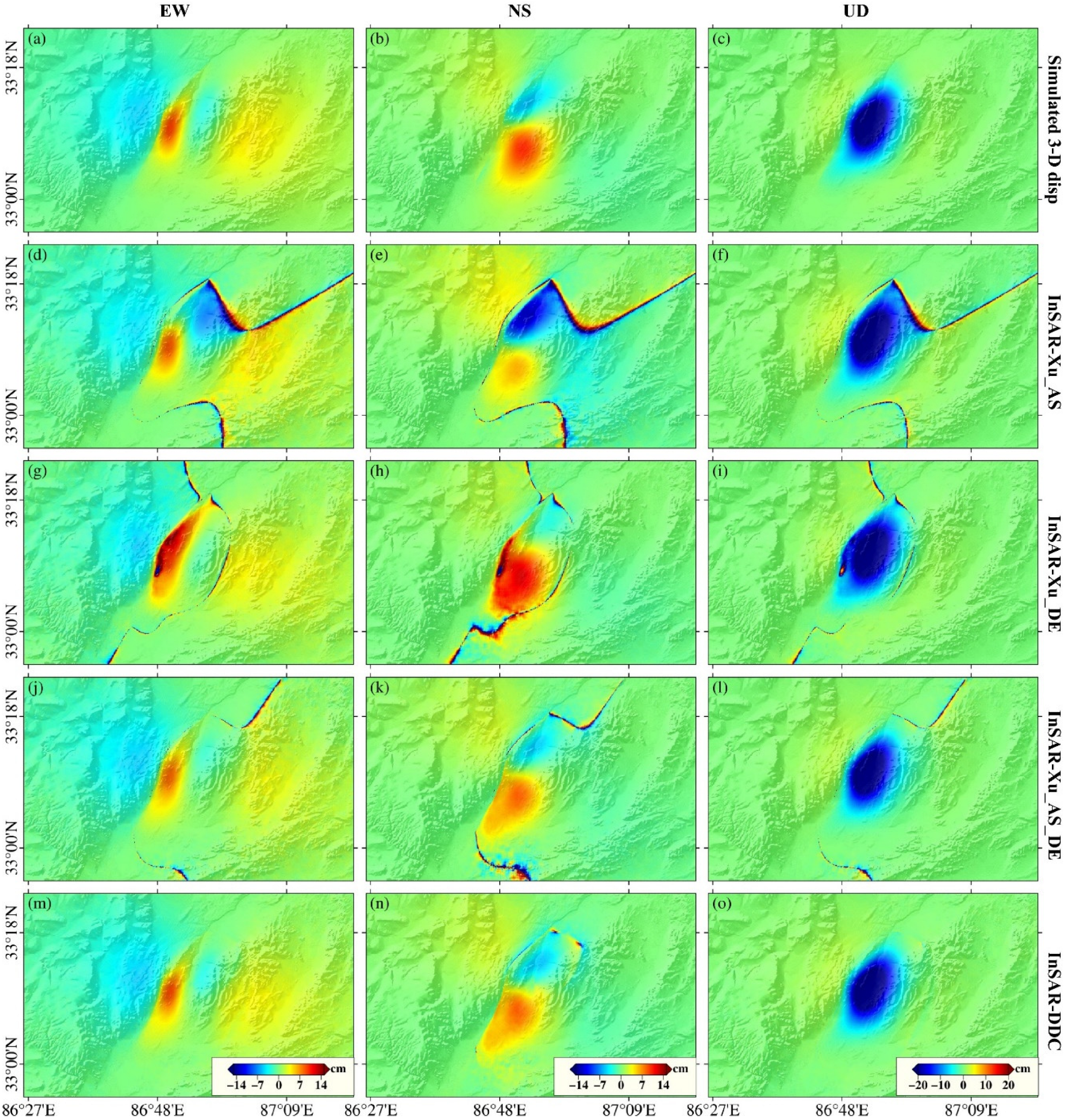[14] (here referred to as the InSAR-Xu method) and the proposed InSAR-DDC method are used to estimate 3D displacements in simulation experiments. Given that one InSAR observation is sufficient to derive co-seismic 3D displacements for the InSAR-Xu method, two 3D displacements can be obtained for the InSAR-Xu method based on ascending (InSAR-Xu_AS) and descending (InSAR-Xu_DE) InSAR observations.

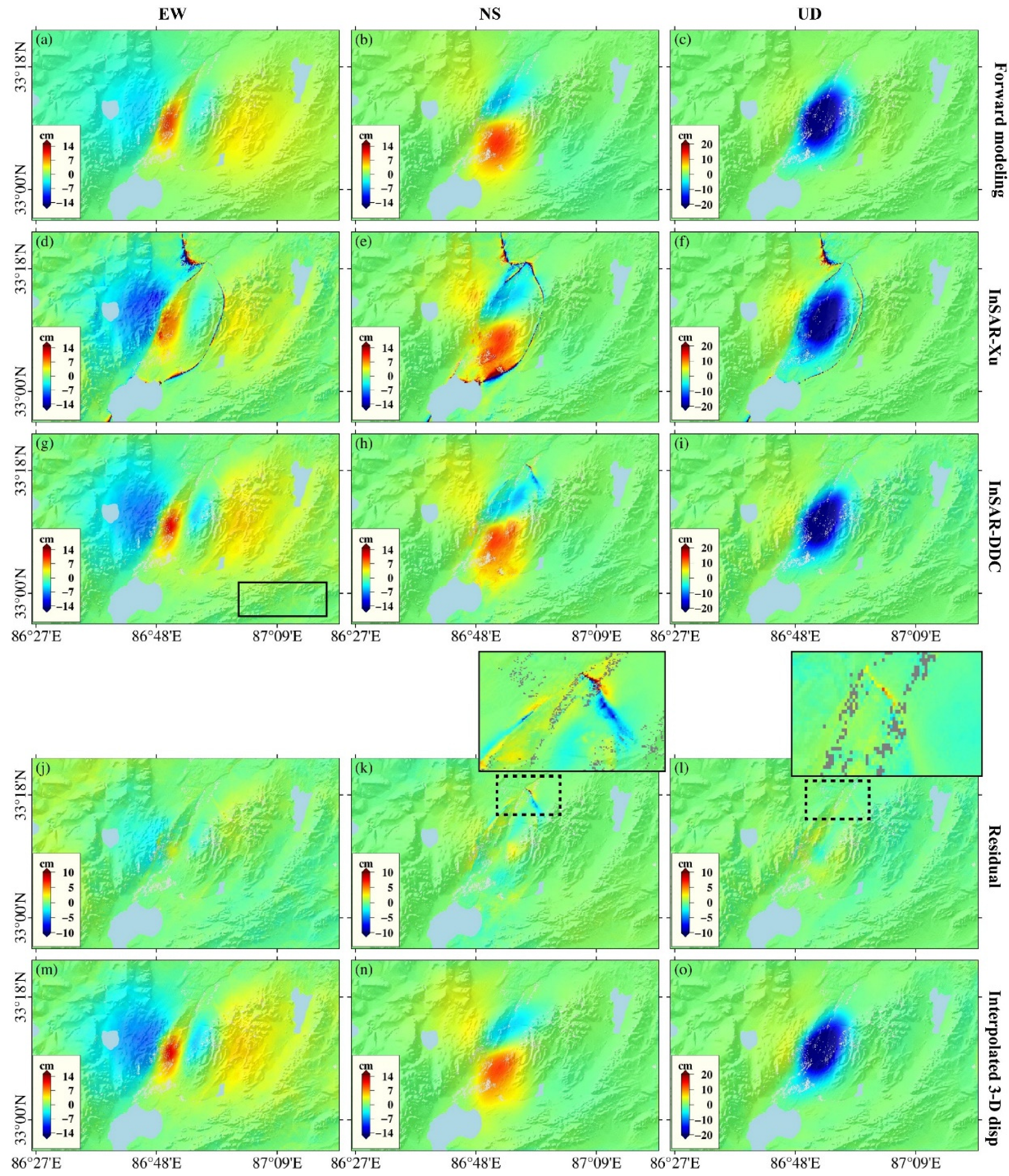
Figure 4 shows the co-seismic 3D displacements obtained by different methods. It can be seen that the results of different methods are overall in good agreement with the simulated 3D displacements (Figure 4a–c). However, the InSAR-Xu-obtained 3D displacements (Figure 4d–l) contain many obvious outliers, and the outlier distribution in InSAR-Xu_AS (Figure 4d–f) and InSAR-Xu_DE (Figure 4g–i) method is quite different. Figure 4j–l shows 3D displacements by combining ascending and descending data based on the InSAR-Xu method (InSAR-Xu_AS_DE), which contain fewer outliers benefitting from the employing of both ascending and descending InSAR observations. The 3D displacements obtained by the proposed InSAR-DDC method (Figure 4m–o) contain the fewest outliers; then they are used and at the same time two virtual observation equations are established to assist the estimation of 3D displacements. In addition, we find from the 3D displacements that the outliers are caused by the insensitivity of the InSAR observations to the displacements in some directions, and in this sense, these methods based on the displacement direction constraint will cause outliers in the 3D displacements. When the horizontal displacement is close to the north–south direction, even if the ascending and descending data are used at the same time, multi-directional constraints and the corresponding levelling process are necessary. Therefore, it can be seen that the results of the InSAR-DDC method contain fewer outliers in contrast to the InSAR-Xu_AS_DE method.

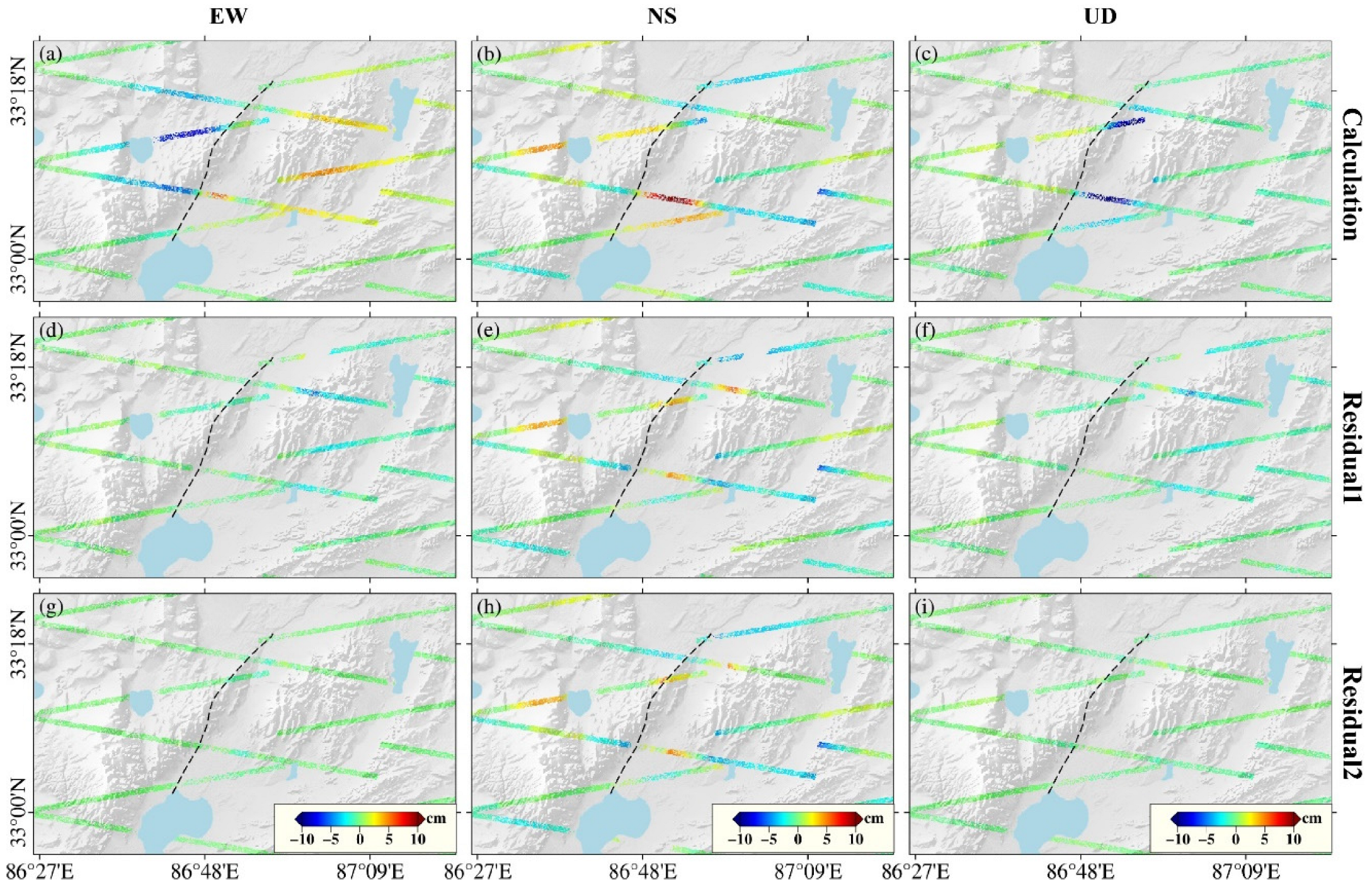
To quantitatively assess the performance of different methods, five precision indexes of the 3D displacements are presented in

Table 1. Five precision indexes of 3D displacements obtained from different methods.

Method	MAX (cm)			MIN (cm)			MEAN (cm)			STD (cm)			RMSE (cm)
	EW	NS	UD	EW	NS	UD	EW	NS	UD	EW	NS	UD	EW	NS	UD
InSAR-Xu_AS	6.30	8.91	5.33	−6.48	−10.74	−6.86	−0.20	−0.35	−0.11	0.84	1.47	0.84	0.87	1.51	0.85
InSAR-Xu_DE	15.45	15.61	3.73	−4.21	−5.67	−13.63	0.20	0.11	−0.17	0.94	1.15	0.81	0.96	1.15	0.83
InSAR-Xu_AS_DE	4.58	4.67	3.99	−4.18	−6.70	−3.70	−0.19	−0.14	−0.05	0.51	0.69	0.41	0.54	0.71	0.41
InSAR-DDC	3.65	4.53	13.74	−1.76	−5.07	−6.10	−0.07	−0.14	0.04	0.30	0.66	0.29	0.31	0.67	0.29

. As can be seen, the accuracies of the 3D displacements provided by the InSAR-Xu_AS and InSAR-Xu_DE methods are lower than the accuracies of the 3D displacements provided by the proposed method. This is expected since only one-track InSAR observations are more sensitive to the observation errors. Furthermore, we also calculate five precision indexes of the 3D displacements of the InSAR-Xu_AS_DE method, and we can note that the RMSE value is significantly decreased compared with the RMSEs of the InSAR-Xu_AS and InSAR-Xu_DE methods, but is still larger than the RMSEs of the 3D displacements by the proposed InSAR-DDC method, which can be attributed to the fact that the new method adds a displacement direction constraint and performs an adjustment process to reduce the effect of errors.

Facing the problem of outliers in the above analysis, according to the theory analysis with the error propagation law and Equation (6), the factor–cofactor matrix of the obtained 3D displacement values can be expressed as

$$Q_{xx}={\left(B^T{P}_{L}B\right)}^{-1}$$

(12)

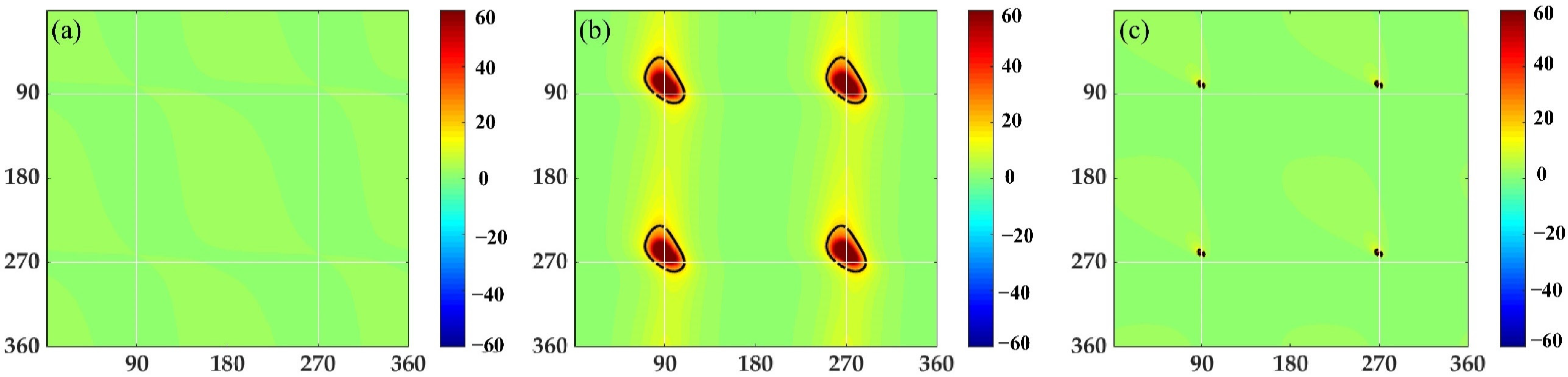
where $P_L$ is the observation weight matrix, $B$ is the coefficient matrix, and the factors of the east–west, north–south, and vertical displacement are the diagonal elements of the matrix $Q_{xx}$. It should be noted that the variance of a variable is equal to factor times variance of unit weight. Since the variance of unit weight is constant for all variables, we only analyze the factor of each component to represent the precision of 3D displacements. Note that the factor is dimensionless. In the paper, the accuracy evaluation is performed using the factor in the factor–cofactor matrix. The corresponding factor maps are shown in Figure 5.

Equation (12) indicates that the precision of the 3D displacements is highly related to the coefficient matrix $B$ when the weight matrix $P_L$ is determined. As for the coefficient matrix $B$, the first two rows can be considered constants for different pixels within the study area since the imaging geometry difference can be negligible. In this case, it is the variety of the last two rows in the matrix $B$ that makes the matrix $B$ and the factor–cofactor matrix $Q_{xx}$ vary for different pixels. More precisely, different 3D displacement directions (i.e., the value of angles $\alpha$ and $\beta$) lead to different values for the last two rows of the matrix $B$. Based on this relationship, the theoretical accuracy (i.e., factor) of the 3D displacements can be calculated for different angles $\alpha$ and $\beta$ based on Equation (12). As shown in Figure 5, the overall accuracy of the east–west displacement is the highest compared with the north–south and vertical components, while, in the factor maps of the north–south and vertical components (Figure 5b,c), four distinct red areas, representing high error, are observed, which likely correspond to the outlier regions in the simulated and real experiments. It can be observed in Figure 5 that large factor values correspond to the displacement direction angles $\alpha$ and $\beta$ of about 90° or 270°. It is just when $\alpha$ and $\beta$ are about 90° or 270° that the ratios $f_1,f_2$ in Equation (4) are infinite. In this case, the matrix $B$ in Equation (6) is rank defect, and a large magnitude of outliers are observed in the final 3D displacements. We discuss the solution for the outliers in detail in the Discussion section.

5. Co-Seismic 3D Displacements of the 2020 Nima Earthquake

This section presents the co-seismic 3D displacements of the 2020 Nima earthquake. Firstly, the DInSAR method was used to obtain the co-seismic displacements of the 2020 Nima earthquake. Based on the DInSAR results, the slip distribution was inverted using the fault dislocation model, and the simulated co-seismic 3D displacements were obtained by forward modeling. The high-precision co-seismic 3D displacements of the 2020 Nima earthquake were calculated based on the ascending/descending data and the proposed InSAR-DDC method.

5.1. DInSAR Displacements

In order to obtain the complete co-seismic displacements of this earthquake, four Sentinel-1A SAR images from ascending/descending tracks were selected for DInSAR processing, and the basic parameters of these SAR data are shown in

Table 2. Basic parameters of the Sentinel-1A SAR data.

Track	Wavelength (cm)	Master Image	Slave Image	Temporal Baseline (Day)	Spatial Perpendicular Baseline (m)
Ascending	5.6	18 July 2020	30 July 2020	12	84.7
Descending	5.6	14 July 2020	26 July 2020	12	−72.3

. The Shuttle Radar Topography Mission DEM (SRTM; resolution 30 m) was used to remove the topographic phase [28]. Interferograms were generated under the multi-look operation of 20:4 (range: azimuth), and the Goldstein filtering method [29] was used to filter the interferogram for decreasing the decorrelation noise. The minimum cost flow method [30] was used to perform the phase unwarping at pixels with the coherence value greater than 0.5.

Figure 6 shows co-seismic LOS displacements of the 2020 Nima earthquake. As can be seen from Figure 6a,d, the fault trace can divide the displacement field into east and west walls. The east and west walls in the ascending observation move in opposite directions. However, in the descending observation, the displacement direction on two walls is the same. The maximum displacements of ~30 cm (away from the satellite) and ~25 cm (away from the satellite) can be observed in the ascending and descending tracks, respectively. In both the ascending and descending tracks, the displacement magnitude and gradient are larger in the east wall compared with those in the west wall, and the overall displacement pattern over the study area is very similar, implying the presence of an east-tilted normal fault. Moreover, no distinct displacement discontinuity can be observed across the east and west walls, indicating that the 2020 Nima earthquake disrupted a buried northeast-trending normal fault.

5.2. Simulated Co-Seismic 3D Displacements Based on Fault Dislocation Model

Before obtaining the simulated co-seismic 3D displacements, it is necessary to extract the slip distribution of the 2020 Nima earthquake. Firstly, the fault trace was identified as a curved fault based on the displacement results and the published articles [18,21]. Secondly, we divided a 38-km-long and 25-km-wide fault plane into 1 km × 1 km small patches. Finally, the Laplace operator was used to constrain the slip roughness [31]. While reaches balanced the trade-off between the squared data misfit and the squared slip roughness, the corresponding smoothing factor is considered to be optimal, and therefore the smoothing factor was set to 0.48 in this experiment. Figure 7 shows the slip distribution obtained by the linear inversion. Based on the obtained slip distribution results, the model-based LOS displacements were also calculated, and the differences between the observed and modeled results are presented in Figure 6. As can be seen, the residuals are quite small, and the RMSEs of the residuals are 0.84 cm and 0.81 cm for the ascending and descending tracks, respectively, indicating that the inversion process based on the fault dislocation model can accurately obtain the fault parameters of the 2020 Nima earthquake. Based on the obtained slip distribution and the fault parameters of the 2020 Nima earthquake, the simulated co-seismic 3D displacements (Figure 8a–c) were calculated by the forward modeling (i.e., Equation (2)). Since the simulated 3D displacements are susceptible to the dislocation model parameter errors, further refinement is necessary.

5.3. Co-Seismic 3D Displacements of the 2020 Nima Earthquake Based on the InSAR-DDC Method

Based on the simulated co-seismic 3D displacements (Figure 8a–c), Figure 8d–f shows a set of 3D displacement results obtained by applying the InSAR_Xu method to the real experiment; the InSAR-DDC method was used to obtain the final high-precision co-seismic 3D displacements of the 2020 Nima earthquake (Figure 8g–i). It can be seen that the 3D displacements obtained by the proposed method have fewer outliers in contrast to the InSAR_Xu method. Figure 8j–l shows the differences between Figure 8g–i and Figure 8a–c. It can be found that, similar to the simulation experiments, some outliers are found in the north–south and vertical displacement maps in the real experiments (Figure 8h,i,k,l), which will be discussed in detail in the Discussion section. Figure 8m–o shows that this earthquake is dominated by the vertical displacement (~32 cm) in the east wall, while only a small magnitude of uplift can be observed in the west wall, which is consistent with the displacement characteristics of the normal fault. The magnitude of horizontal displacement is relatively small compared with the vertical component, and the maximum horizontal displacement of ~12 cm occurred near the center of significant vertical displacement. For quantitative assessment of the 3D displacements calculated from the InSAR-DCC method, an area far from the deformed region is selected (the rectangle in Figure 8g), where the displacement can be assumed to be zero. The RMSEs of 3D displacements in this area are calculated as 0.94 cm, 0.50 cm, and 0.19 cm for the east–west, north–south, and vertical components, respectively. This result can validate the accuracy of the proposed InSAR-DDC method to some extent when there is no external geodetic observation available.

6. Discussion

In this section, the solution for the outliers in the 3D displacements are first presented. In addition, since there is no external geodetic displacement observation available for InSAR result accuracy assessment, we tried to derive the azimuth displacements by the BOI method. Although the BOI displacements are only available within the burst overlap (BO) regions of the Sentinel-1A data, they can be used as an independent dataset for accuracy assessment. Finally, the co-seismic displacements and fault movement characteristics of the 2020 Nima earthquake are analyzed based on the InSAR-DDC-obtained 3D displacements.

6.1. The Solution for the Outliers in the Co-Seismic 3D Displacements

Xu et al. [14] calculated the 3D displacement vector directions based on the forward modeling 3D displacements, then obtained the final 3D displacements of the 2008 Wenchuan earthquake by combining a single-track InSAR-LOS observation and the vector direction constraint. Since the seismologic fault of the 2008 Wenchuan earthquake is striking NE–SW with thrust and a right-lateral components fault [32,33], the InSAR observation of the near-polar orbit has good sensitivity to most of the co-seismic displacements of this earthquake, and the outliers are hardly observed in the case study of the 2008 Wenchuan earthquake. However, when the near north–south displacement dominates the horizontal ground movement, to which the InSAR observations are insensitive, the outliers appear in the final 3D displacements. Therefore, in the 2020 Nima earthquake case study, we aim to analyze the cause of the outliers and to find a solution for mitigating the outliers in the final co-seismic 3D displacements.

The theoretical analysis in simulation experiments is consistent with the Nima earthquake experiment results in that the obtained north–south and vertical displacements (Figure 8h,i) contain obvious outliers and the corresponding factor maps (Figure 5b,c) also show large values. To mitigate the outliers in the 3D displacements, we propose to mask the outlier-prone regions and then to interpolate the void pixels based on the surround valid displacements, in which the key step is to mask the outlier-prone regions. According to the factor map calculated in the simulation experiment, the relationship between the displacement direction angles $\alpha$ and $\beta$ and the accuracy factor is clearly shown in Figure 5. Now, the key point is to determine the factor threshold $e$. In the experiment, in order to mask the outliers as much as possible, we set the factor threshold $e$ to 20 after many attempts. We believe that when the factor is greater than 20, the corresponding angle range is sensitive, and outliers will appear in the corresponding 3D displacements results. Generally speaking, the selection of thresholds is determined by the range of outliers, and the selection of the factor threshold is based on the number of outliers, which requires finding sensitive angles and masking the outlier regions as much as possible. After masking the outlier regions, the Kriging interpolation is performed on the void pixels based on the surround valid displacements, which guarantees the completeness and the accuracy of the InSAR-DDC-obtained co-seismic 3D displacements. Based on this outlier solution, the initial obtained 3D displacements are improved (Figure 8m–o), in which no outlier can be observed, and the results are more accurate.

6.2. Accuracy Assessment for Co-Seismic 3D Displacements Based on BOI Observations

In this section, the BOI observations are used as an independent dataset to assess the accuracy of the obtained co-seismic 3D displacements. As shown in Figure 9, there are obvious azimuth displacement signals in the BOI maps, especially around both sides of the fault trace. Since the BOI displacements are available only in the BO regions, the 3D displacements in these BO regions (Figure 10a–c) can be calculated by combining ascending/descending DInSAR and BOI observations with the WLS method. In this case, the 3D displacements in BO regions can be used to assess the accuracy of the InSAR-Xu- or InSAR-DDC-obtained 3D displacements. Figure 10d–i show the residuals of 3D displacements obtained by the InSAR-Xu and InSAR-DDC methods with respect to the 3D displacements obtained by the DInSAR and BOI observations (Figure 10a–c). It can be seen that the residual magnitudes of the east–west and vertical displacements are relatively small compared with the north–south component. This may be attributed to the fact that the BOI observations are more sensitive to decorrelation noise and prone to be affected by the ionospheric disturbs, which in turn would lead to larger errors in the north–south displacement component. For quantitative assessment,

Table 3. The RMSEs of the residuals of the 3D displacements obtained from different methods.

Method	RMSE (cm)
	EW	NS	UD
InSAR-Xu	0.29	0.47	0.28
InSAR-DDC	0.08	0.47	0.11

presents the RMSEs of the 3D displacement residuals (i.e., Figure 10d–i), revealing that the proposed InSAR-DDC method can achieve a higher accuracy of co-seismic 3D displacements compared with the traditional InSAR-Xu method.

6.3. The Surface Deformation Characteristics of the 2020 Nima Earthquake

The north–south and the east–west displacement components are combined to obtain the horizontal displacement vectors of the earthquake, which are down-sampled and shown in Figure 11 (i.e., the red arrows). Results show that the horizontal displacement field can be roughly divided into three regions: left, center, and right. In the left part, the displacement is toward the northwest with a slight uplift; in the center part, the displacement characteristics are similar to those of a subsidence funnel that the horizontal displacements point to the subsidence center; and in the right part, the displacement is toward the east direction with negligible vertical displacement. The displacement characteristics indicate that the left and right parts experienced tension stress, while the center part experienced extrusion stress. The co-seismic 3D displacements can intuitively reflect the real surface displacement of the Nima earthquake, and also reflect the geological and tectonic movement to a certain extent.

The InSAR inversion results show almost no significant slip in the shallow crust above a depth of 3 km, which is consistent with the observed surface displacement. A previous study [34] summarized and generalized the nature of active faults in Tibet and concluded that earthquakes of magnitude 5 or higher occurring in Tibet have good correlation with active faults on the surface. The 2020 Mw6.3 Nima earthquake occurred on the northern side of the Bangong Lake–Nujiang suture zone, the Qiangtang block in the Tibetan Plateau, where the plate is prone to tensile ruptures during the uplift of the Tibetan Plateau. Since the Tibetan Plateau is also accompanied with the N–S-striking normal rupture and NE-striking sinistral rupture, there are different geomorphic features of the linear and narrow valley and much shorter and wider grabens around the study area.

The source mechanism and the obtained 3D displacements show that this earthquake is a normal tensional rupture, which is consistent with the overall displacement pattern of the Qiangtang block. This earthquake occurred in the RYJ, which has an overall NE trend and is a left-lateral strike-slip-oriented rupture with some tensional activity in the local area, and the Yibu Chaka garden is bounded by two master normal faults (west and east Yibu Chaka faults). Inversion results, fault kinematics, and regional geology geomorphology indicate that the source of the Nima earthquake is the deep part of the west Yibu Chaka normal fault (shown in Figure 1), which is located in the middle part of the RYJ fault zone (shown in Figure 1). The central segment of the RYJ fault zone is characterized by N to NNE-striking normal faults. Although the maximum slip extent of the RYJ fault remains unknown, the minimum length of 300 km is accepted. Fault orientation and kinematics change in topographic relief, which is about 500 m along the strike-slip portion of the fault zone and increases to more than 1000 m in the normal fault portion [35].

7. Conclusions

In this paper, we proposed a method to calculate co-seismic 3D displacements from InSAR observations with the dislocation model-based displacement direction constraint, termed by the InSAR-DDC method. The method firstly obtains simulated co-seismic 3D displacements by inverse and forward modeling based on the fault dislocation model and InSAR observations. Two virtual observation equations can then be established from the simulated 3D displacements under the situation that the directions of simulated and real 3D displacements are very similar. Finally, the high-precision co-seismic 3D displacements can be calculated by combining ascending/descending InSAR observations and two virtual observation equations based on the WLS method. Both the simulations and real experiment of the 2020 Nima earthquake demonstrated that the proposed InSAR-DDC method can obtain a higher accuracy of co-seismic 3D displacements compared with the traditional methods.

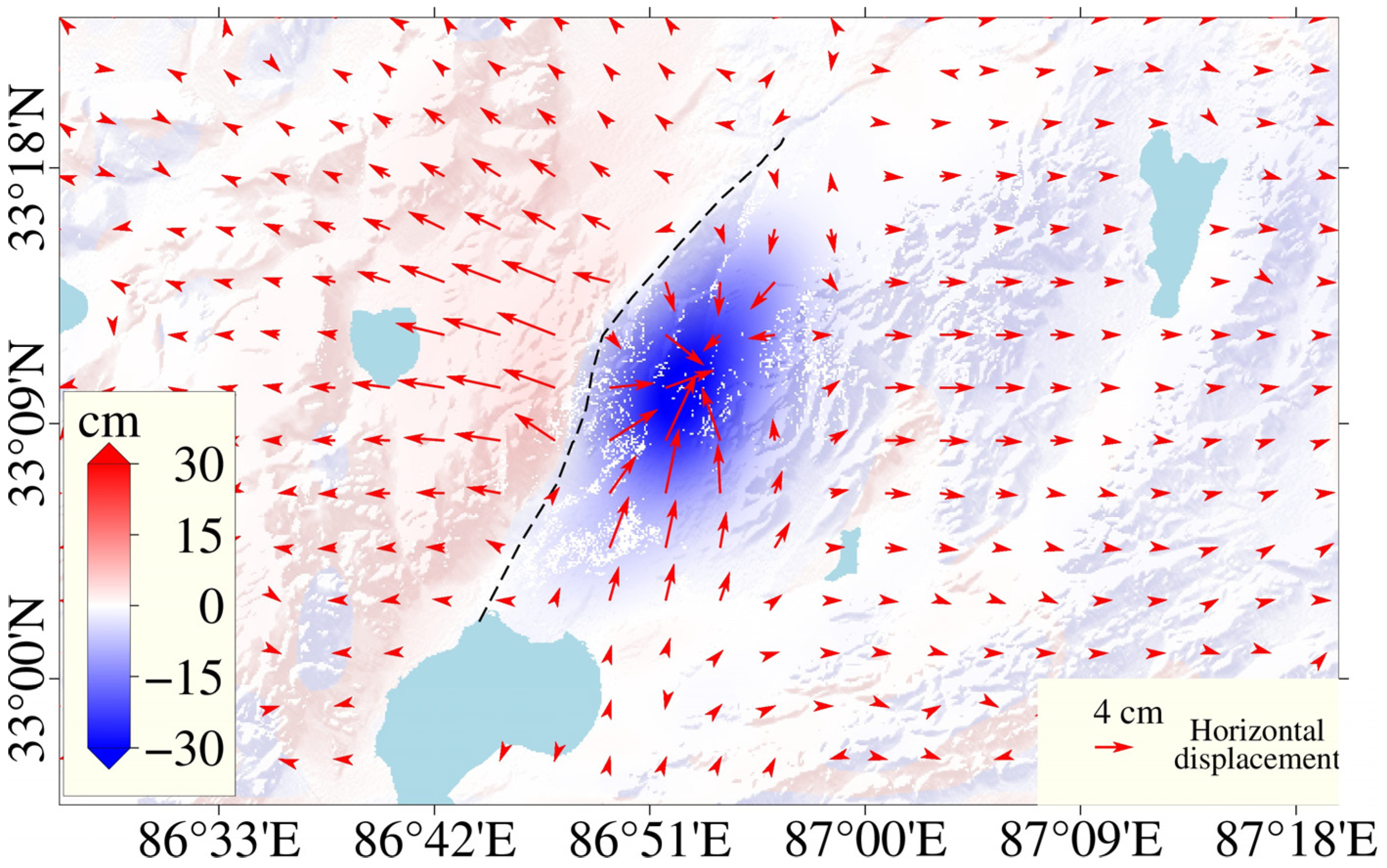
At the same time, this paper found that the methods with displacement direction constraint are highly prone to outliers when solving 3D displacements with special displacement directions. We looked through the cause of the outliers and proposed a solution to mitigate the outliers in the 3D displacements; then the final high-precision co-seismic 3D displacements of the 2020 Nima earthquake were obtained. The co-seismic 3D displacements indicate that the seismologic fault is the west Yibu Chaka normal fault, and the vertical displacement dominates the surface displacements with the maximum magnitude of ~32 cm. In general, the displacement area of this earthquake can be divided into the left, center, and right parts, where the left and right parts experienced tension stress and the center part experienced extrusion stress, and the overall displacement pattern fits well with the tensile rupture.

The proposed InSAR-DDC method in this paper establishes virtual observation equations based on the fault dislocation model, and then combines InSAR observations to estimate the co-seismic 3D displacements with the WLS method. This process can provide additional constraint equations with respect to 3D displacements based on the essential geophysical model, and overcome the dilemma that only ascending and descending DInSAR observations cannot calculate 3D displacements. Actually, the dataset deficiency situation is very common for current InSAR 3D displacement measurements; therefore, the strategies proposed in this paper can provide a reference for the InSAR 3D displacement measurements with respect to other geohazards.

References

1. Gabriel, A.K.; Goldstein, R.M.; Zebker, H.A. Mapping small elevation changes over large areas: Differential radar interferometry. J. Geophys. Res. Solid Earth 1989, 94, 9183–9191. [Google Scholar] [CrossRef]
2. Michel, R.; Avouac, J.P.; Taboury, J. Measuring ground displacements from SAR amplitude images: Application to the Landers earthquake. Geophys. Res. Lett. 1999, 26, 875–878. [Google Scholar] [CrossRef]
3. Bechor, N.B.D.; Zebker, H.A. Measuring two-dimensional movements using a single InSAR pair. Geophys. Res. Lett. 2006, 33, 16. [Google Scholar] [CrossRef]
4. Grandin, R.; Klein, E.; Metois, M.; Vigny, C. Three-dimensional displacement field of the 2015 M(w)8.3 Illapel earthquake (Chile) from across- and along-track Sentinel-1 TOPS interferometry. Geophys. Res. Lett. 2016, 43, 2552–2561. [Google Scholar] [CrossRef]
5. Hu, J.; Liu, J.; Li, Z.; Zhu, J.; Wu, L.; Sun, Q.; Wu, W. Estimating three-dimensional coseismic deformations with the SM-VCE method based on heterogeneous SAR observations: Selection of homogeneous points and analysis of observation combinations. Remote Sens. Environ. 2021, 255, 112298. [Google Scholar] [CrossRef]
6. Jung, H.S.; Lu, Z.; Won, J.S.; Poland, M.P.; Miklius, A. Mapping Three-Dimensional Surface Deformation by Combining Multiple-Aperture Interferometry and Conventional Interferometry: Application to the June 2007 Eruption of Kilauea Volcano, Hawaii. IEEE Geosci. Remote Sens. Lett. 2011, 8, 34–38. [Google Scholar] [CrossRef]
7. Liu, J.; Hu, J.; Li, Z.; Ma, Z.; Shi, J.; Xu, W.; Sun, Q. Three-Dimensional Surface Displacements of the 8 January 2022 Mw6.7 Menyuan Earthquake, China from Sentinel-1 and ALOS-2 SAR Observations. Remote Sens. 2022, 14, 1404. [Google Scholar] [CrossRef]
8. Liu, J.; Hu, J.; Li, Z.; Ma, Z.; Zhu, J. Complete three-dimensional coseismic displacements related to the 2021 Maduo earthquake in Qinghai Province, China from Sentinel-1 and ALOS-2 SAR images. Sci. China Earth Sci. 2022, 65, 687–697. [Google Scholar] [CrossRef]
9. Hu, J.; Li, Z.W.; Ding, X.L.; Zhu, J.J.; Zhang, L.; Sun, Q. Resolving three-dimensional surface displacements from InSAR measurements: A review. Earth-Sci. Rev. 2014, 133, 1–17. [Google Scholar] [CrossRef]
10. Pepe, A.; Solaro, G.; Calo, F.; Dema, C. A Minimum Acceleration Approach for the Retrieval of Multiplatform InSAR Deformation Time Series. IEEE J. Sel. Top. Appl. Earth Obs. Remote Sens. 2016, 9, 3883–3898. [Google Scholar] [CrossRef]
11. Qu, C.; Qiao, X.; Shan, X.; Zhao, D.; Zhao, L.; Gong, W.; Li, Y. InSAR 3-D Coseismic Displacement Field of the 2015 Mw 7.8 Nepal Earthquake: Insights into Complex Fault Kinematics during the Event. Remote Sens. 2020, 12, 3982. [Google Scholar] [CrossRef]
12. Song, X.; Jiang, Y.; Shan, X.; Qu, C. Deriving 3D coseismic deformation field by combining GPS and InSAR data based on the elastic dislocation model. Int. J. Appl. Earth Obs. Geoinf. 2017, 57, 104–112. [Google Scholar] [CrossRef]
13. Xu, K.; Gan, W.; Wu, J.; Hou, Z. A robust method for 3-D surface displacement fields combining GNSS and single-orbit InSAR measurements with directional constraint from elasticity model. GPS Solut. 2022, 26, 46. [Google Scholar] [CrossRef]
14. Xu, K.; Sun, W.; Wu, J. A New Method for Constructing 3-D Crustal Deformation Field From Single InSAR-LOS Data. IEEE Geosci. Remote Sens. Lett. 2021, 19, 4000505. [Google Scholar] [CrossRef]
15. Deng, Q.D.; Gao, X.; Chen, G.H. Recent tectonic activity of Bayanhar fault block and the Kunlun-Wenchuan earthquake series of the Tibetan Plateau. Earth Sci. Front. 2010, 17, 163–178. [Google Scholar]
16. Liang, X.; Wang, G.; Yuan, G.; Liu, Y. Structural sequence and geochronology of the Qomo Ri accretionary complex, Central Qiangtang, Tibet: Implications for the Late Triassic subduction of the Paleo-Tethys Ocean. Gondwana Res. 2012, 22, 470–481. [Google Scholar] [CrossRef]
17. Li, C.T.; Li, Q.; Tan, K. Coseismic deformation characteristics of the 2020 Nima, Xizang Mw6.3 earthquake from Sentinel-1A/B InSAR data and rupture slip distribution. Chin. J. Geophys. 2021, 64, 2297–2310. [Google Scholar] [CrossRef]
18. Gao, H.; Liao, M.; Liang, X.; Feng, G.; Wang, G. Coseismic and Postseismic Fault Kinematics of the July 22, 2020, Nima (Tibet) Ms6.6 Earthquake: Implications of the Forming Mechanism of the Active N-S-Trending Grabens in Qiangtang, Tibet. Tectonics 2022, 41, e2021TC006949. [Google Scholar] [CrossRef]
19. Huang, Y.T.; Li, W.; Jiang, X. Co-seismic deformation field of the 2020 Nima Tibet Earthquake and fault slip distribution. Bull. Surv. Mapp. 2021, 2021, 173–177. [Google Scholar] [CrossRef]
20. Yang, J.Y.; Xu, C.J.; Wen, Y.M.; Xu, G.Y. The July 2020 Mw 6.3 Nima Earthquake, Central Tibet: A Shallow Normal-Faulting Event Rupturing in a Stepover Zone. Seismol. Res. Lett. 2021, 93, 45–55. [Google Scholar] [CrossRef]
21. Li, K.; Li, Y.; Tapponnier, P.; Xu, X.; Li, D.; He, Z. Joint InSAR and Field Constraints on Faulting During the Mw 6.4, July 23, 2020, Nima/Rongma Earthquake in Central Tibet. J. Geophys. Res.-Solid Earth 2021, 126, e2021JB022212. [Google Scholar] [CrossRef]
22. Feng, W.; Li, Z.; Elliott, J.R.; Fukushima, Y.; Hoey, T.; Singleton, A.; Cook, R.; Xu, Z. The 2011 M-W 6.8 Burma earthquake: Fault constraints provided by multiple SAR techniques. Geophys. J. Int. 2013, 195, 650–660. [Google Scholar] [CrossRef]
23. Liu, J.; Hu, J.; Xu, W.; Li, Z.; Zhu, J.; Ding, X.; Zhang, L. Complete Three-Dimensional Coseismic Deformation Field of the 2016 Central Tottori Earthquake by Integrating Left- and Right-Looking InSAR Observations With the Improved SM-VCE Method. J. Geophys. Res.-Solid Earth 2019, 124, 12099–12115. [Google Scholar] [CrossRef]
24. Fialko, Y.; Sandwell, D.; Simons, M.; Rosen, P. Three-dimensional deformation caused by the Bam, Iran, earthquake and the origin of shallow slip deficit. Nature 2005, 435, 295–299. [Google Scholar] [CrossRef]
25. He, P.; Wen, Y.; Xu, C.; Chen, Y. High-quality three-dimensional displacement fields from new-generation SAR imagery: Application to the 2017 Ezgeleh, Iran, earthquake. J. Geod. 2019, 93, 573–591. [Google Scholar] [CrossRef]
26. Hu, J.; Ding, X.; Zhang, L.; Sun, Q.; Li, Z.; Zhu, J.; Lu, Z. Estimation of 3-D Surface Displacement Based on InSAR and Deformation Modeling. IEEE Trans. Geosci. Remote Sens. 2017, 55, 2007–2016. [Google Scholar] [CrossRef]
27. Wang, T.; Jonsson, S. Improved SAR Amplitude Image Offset Measurements for Deriving Three-Dimensional Coseismic Displacements. IEEE J. Sel. Top. Appl. Earth Obs. Remote Sens. 2015, 8, 3271–3278. [Google Scholar] [CrossRef]
28. Farr, T.G.; Rosen, P.A.; Caro, E.; Crippen, R.; Duren, R.; Hensley, S.; Kobrick, M. The shuttle radar topography mission. Rev. Geophys. 2007, 45, 2. [Google Scholar] [CrossRef]
29. Goldstein, R.M.; Werner, C.L. Radar interferogram filtering for geophysical applications. Geophys. Res. Lett. 1998, 25, 4035–4038. [Google Scholar] [CrossRef]
30. Carballo, G.F.; Fieguth, P.W. Probabilistic cost functions for network flow phase unwrapping. IEEE Trans. Geosci. Remote Sens. 2000, 38, 2192–2201. [Google Scholar] [CrossRef]
31. Harris, R.A.; Segall, P. Detection of a locked zone at depth on the Parkfield, California, segment of the San Andreas Fault. J. Geophys. Res. Solid Earth 1987, 92, 7945–7962. [Google Scholar] [CrossRef]
32. Fukuyama, E.; Hao, K.X. Subparallel Dipping Faults that Ruptured during the 2008 Wenchuan Earthquake. Bull. Seismol. Soc. Am. 2013, 103, 2128–2134. [Google Scholar] [CrossRef]
33. Wen, Y.; Xu, C.; Li, Z.; Liu, Y.; Feng, W.; Shan, X. Coseismic and postseismic deformation of the 2008 Wenchuan Earthquake from InSAR. Chin. J. Geophys. 2014, 57, 1814–1824. [Google Scholar] [CrossRef]
34. Taylor, M.; Yin, A. Active structures of the Himalayan-Tibetan orogen and their relationships to earthquake distribution, contemporary strain field, and Cenozoic volcanism. Geosphere 2009, 5, 199–214. [Google Scholar] [CrossRef]
35. Taylor, M.; Yin, A.; Ryerson, F.J.; Kapp, P.; Ding, L. Conjugate strike-slip faulting along the Bangong-Nujiang suture zone accommodates coeval east-west extension and north-south shortening in the interior of the Tibetan Plateau. Tectonics 2003, 22, 4. [Google Scholar] [CrossRef] [Green Version]
Figure 1. Tectonic map of the 2020 Mw6.3 Nima earthquake. (a) Color-shaded relief map. The solid rectangles represent the footprints of the used SAR data. The white dashed rectangle outlines the study area. The black lines are the location of mapped faults. The red line represents the fault trace of this event identified in this paper. The red beach ball and the red star are the focal mechanism and the epicenter of the 2020 Nima earthquake, respectively. The blue square is Nima county. The Riganpei Co–Yibu Chaka–Jiangaizangbu fault system consists of the West Yibug Caka fault (WYF), Riganpei Co fault (RCF), Jiangaizangbu fault (JF), and Yibug Caka–Riganpei co fault (YRF). The grey triangle represents the basin between the WYF and RCF faults. (b) The tectonic setting around the study area. The red dashed lines are the mapped faults. The white dashed rectangle indicates the range of (a). The insert map shows the location of Nima county (the blue star) in China. The blue arrow denotes the northeastward movement (28 ± 5 mm/a) of the Qiangtang block. The blue square is Nima county. White circles are four historic Mw > 7.0 earthquakes and yellow circles are historic Mw > 6.0 earthquakes between 1997 and 2022.
Remotesensing 14 04481 g001
Figure 2. The flowchart of the proposed method.
Remotesensing 14 04481 g002
Figure 3. Simulated (a) ascending and (b) descending InSAR observations in simulation experiments.
Remotesensing 14 04481 g003
Figure 4. Three-dimensional displacements obtained by different methods in the simulation experiments. (ac) The simulated 3D displacements (i.e., the truth). (df) and (gi) are the 3D displacements obtained by the InSAR-Xu method based on ascending and descending InSAR observations (InSAR-Xu_AS and InSAR-Xu_DE), respectively. (jl) are the 3D displacements obtained by the InSAR-Xu method based on ascending and descending InSAR observations (InSAR-Xu_AS_DE). (mo) are the 3D displacements obtained by the proposed InSAR-DDC method based on ascending and descending InSAR observations.
Remotesensing 14 04481 g004
Figure 5. The factor of 3D displacements versus displacement direction angles α ,   β . (ac) are the east–west, north–south, and vertical components, respectively. The x-axis and y-axis represent angles α and β , respectively. The black dashed lines in (b,c) correspond to the factor threshold e . The light white lines represent 90° or 270°.
Remotesensing 14 04481 g005
Figure 6. Observations and modeled LOS displacements are shown in the left and middle column, respectively. Residuals are shown in right column. Panels (ac) show the ascending track; panels (df) show the descending track. The light blue area is the lake, the black dashed line is fault trace identified in this paper.
Remotesensing 14 04481 g006
Figure 7. Slip distribution of the 2020 Nima earthquake in (a) 3D and (b) 2D views. The size of each patch is 1 km × 1 km.
Remotesensing 14 04481 g007
Figure 8. 3D displacement components and residuals of the 2020 Nima earthquake. (ac) are the 3D displacements obtained by forward modeling; (df) are the 3D displacements obtained by the InSAR-Xu method; (gi) are the 3D displacements obtained by the InSAR-DDC method; (jl) are the corresponding residuals of (gi) with respect to (ac); (mo) are the interpolated 3D displacements by the kriging method. The black rectangle in (g) shows the far-field area where the displacements are assumed to be zero. The insert maps in the upper right corner of (k,l) show details in the corresponding black dashed rectangles. The light blue regions are the water area.
Remotesensing 14 04481 g008
Figure 9. (a) ascending and (b) descending BOI-obtained azimuth displacements. The black dashed line is the fault trace identified in this paper.
Remotesensing 14 04481 g009
Figure 10. Three-dimensional displacements within the burst overlap regions obtained from different methods. (ac) Calculation: the direct WLS calculation based on the ascending/descending DInSAR and BOI observations. (df) Residual1: the residuals of 3D displacements from InSAR-Xu method with respect to (ac). (gi) Residual2: the residuals of 3D displacements from the proposed InSAR-DDC method with respect to (ac). The black dashed line is fault trace identified in this paper.
Remotesensing 14 04481 g010
Figure 11. Co-seismic 3D displacement field of the Nima earthquake. The colored background shows the vertical displacement field, and red arrows indicate the down-sampled horizontal displacements. The length of the arrow represents the magnitude of the horizontal displacements. The black dashed line is the fault trace identified in this paper.
Remotesensing 14 04481 g011