Development of a Multi-Scale Tomato Yield Prediction Model in Azerbaijan Using Spectral Indices from Sentinel-2 Imagery

Abstract

This paper presents the development and update of a multi-scale yield prediction model for processing tomatoes. The study was carried out under the EU-funded programme “Support to Development of a Rural Business Information System (RBIS)”, and the performance of the updated crop-specific yield prediction models and their generated predictions at regional and national levels are presented. The model was built using Sentinel-2 satellite imagery to obtain cumulative values of six (6) selected vegetation indices (VIs). The data were collected on five (5) different dates for processing tomato fields in the Khachmaz region of Azerbaijan during summer 2021 (June to August) at 10- to 13-day intervals. In addition, a targeted field sampling campaign was conducted on selected Khachmaz pilot fields towards the end of the growing season to assess the potential of Sentinel-2 data to determine yield variability in tomato fields. Finally, actual recorded yields were collected at the field level to build the yield prediction regression model and evaluate its performance at different spatial scales, ranging from single field to national level, as well as under different data availability scenarios (number of consecutive Sentinel-2 images used). The results showed a high degree of correlation between all implemented VIs and processing tomato yield, with a coefficient of determination of up to 0.89 for the NDVI, providing valuable information for future estimates of tomato production across multiple spatial scales. The developed prediction model could also be used in the agri-food sector for national yield estimates to support policy and regulatory decisions at the national level.

1. Introduction

Agriculture has always played an important role in the history of Azerbaijan. Climatic and topographical conditions favour the cultivation of a variety of crops, with half of the country classified as mountainous and 18% of the land lying below sea level. Currently, agriculture generates approximately 6% of Azerbaijan’s GDP [1]. A key element of Azerbaijan’s agricultural sector is that it is highly fragmented and includes a large number of small farmers [2]. The number of agricultural producers in 2015 was 1.2 million, with all of them cultivating less than 2.2 million hectares of land in total. In addition, there are over 1200 state-owned and cooperative farms nationwide. Most of Azerbaijan’s cultivated land (over 1 million hectares) is irrigated. Following an oil price crisis in 2016 and the downward trend of the country’s fossil oil and natural gas prices ever since [1], the government has recently adopted a series of strategies to strengthen the agricultural sector. The government’s goal is to improve the business climate for the development of a competitive Azerbaijani agrifood sector, to ensure the country’s food security and to economically empower the rural population.

Early estimates of crop yields enable farmers to optimise their farm planning, field management and product marketing decisions. Data-driven decisions allow for more informed decisions on optimising inputs (e.g., fertilisers, pesticides and water), determining the optimal harvesting method and timing, and most importantly, planning logistics related to product storage, transport and marketing. Therefore, yield estimates serve as an assessment tool for the expected income of each production unit and at the same time enable an efficient transfer of production from the farm to the food supply chain. In remote areas, where the logistics of transporting produce often need to be arranged in advance to plan transport to warehouses, which are often located close to urban centres, information on early yield forecasts can minimise potential risks and ensure optimal handling and storage of produce. For open-field crops, which are grown in the lowlands and therefore often have to travel shorter distances to storage units, the real critical factor for production safety is the storage itself. For high-value crops, and especially produce that is very susceptible to post-harvest quality degradation and has a very short life if left exposed, should be scheduled to be stored several weeks before the product arrives. In addition, the policy of any country can be greatly influenced by yield estimates, the two most important factors for these forecasts being their accuracy and how early they can be made. The importance of yield estimates is even greater in countries where agriculture is the main source of economic activity. Early forecasts can warn decision-makers of potential crop losses so that they can adjust their import and export decisions in time each season and avert a potential food shortage. In the agriculture of the digital age, data is the most valuable currency and the question of “how early” it becomes accessible is the decisive production factor.

Remote sensing encompasses a range of advanced technologies and data analysis techniques that provide a vast amount of information on key agricultural parameters, including crop type, crop status and yields, from the field level to larger geographical areas such as countries or continents. In various case studies, remote sensing applications have been used and evaluated for decision making in irrigation [3,4,5], fertilisation [6] and pesticide use [7,8] to minimise water and nutrient losses and other negative environmental impacts of agricultural practises. Today, the phenological development of crops during a seasonal cycle can be easily monitored from space. In combination with other data sources, stressed regions can be identified and crop yield estimates can be made. Satellite sensors have transformed agricultural activities by providing a timely and accurate picture of the agricultural sector, as they are capable of collecting information over large areas with high repetition frequency [9]. The high resolution of Sentinel-2 has revolutionised crop monitoring and offers immense potential for agricultural management, especially in delineating management zones [6], optimising agricultural inputs and predicting yields [10].

The large spatial coverage and high temporal repetition frequency of satellite imagery make it particularly useful for obtaining near real-time information at the regional level. As it is a cost-effective technology, users can minimise field observations and a large number of users can share the same data [11]. By using seasonal time series of satellite imagery, various phenological indicators, such as the beginning, peak and end of a crop cycle, can be modelled by specific vegetation indices (VIs). The latter are commonly used for crop phenotyping to assess the physiological state of plants under abiotic stress in different crops [12,13,14]. Among VIs, the Normalised Difference Vegetation Index (NDVI) is the most widely used for estimating biomass production, plant vigour, stress level, yield and even as a proxy for photosynthesis [15,16]. In recent years, several approaches to the quantitative estimation of plant productivity parameters have been elaborated, including methods ranging from simple regression equations [17] to the use of more complex plant growth models [18]. Tucker et al., 1980 [19] were among the first researchers to establish a relationship between NDVI and crop yield using experimental fields and ground-based spectral radiometer measurements. Thereafter, numerous studies have reported the good correlation between vegetation indices provided by RS and crop yield and biomass [20,21,22].

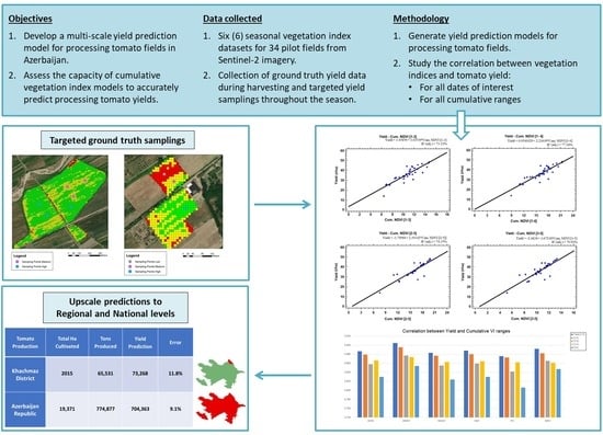
Considering that global tomato production has increased to 186.8 million tonnes by 2020 (FAOSTAT, 2020), the social and economic importance of tomato at the international level is obvious. In Azerbaijan, the tomato production sector has occupied a prominent position among the branches of the country’s agricultural economy for many years. From 2007 to 2018, Azerbaijan achieved the highest growth rate in exports among the main exporting countries. In 2020, the country produced 774,877 tonnes of the raw product, while 19,371 ha were cultivated (FAOSTAT, 2020). Given the great importance of this particular crop and the limited research on this type of cultivation, satellite data were used in this study and NDVI-based work was produced to assess the potential to provide valuable information on tomato processing. Predictive yield maps can be used as spatial databases for the implementation of variable rate cropping (VRT) systems to achieve precise application of field-level inputs to optimise production across the field, especially for high-value crops such as tomato. Gianquinto et al., 2011 [12] investigated yield prediction for tomato using different vegetation indices based on crop reflectance. Koller and Upadhyaya (2005) [23] used a vegetation index based on plant greenness and found it to be reliable for evaluating the yield of processing tomatoes. As reported [15], NDVI is a good estimator for predicting yield and can be used to plan the best time to harvest and transport for industrial processing.

In this study, the capacity of Sentinel-2 imagery to assess canopy growth, yield and field cultivation of tomato crops was evaluated. We used six (6) vegetation indices to extend the approach for early crop yield prediction and to investigate the predictive power of the developed models. A stepwise linear regression method was implemented to select the linear models based on the statistical evaluation of their fit for the entire data set, creating simple equations with easily interpretable coefficients that can forecast crop yield. The inclusion of remote sensing data is carried out to evaluate whether NDVI variables can successfully and accurately quantify yield performance of processing tomatoes at both regional and national levels. A novelty is the use of different cumulative NDVI ranges as predictors in statistical modelling, as satellite data availability is often limited (not constant availability of products in the desired temporal frequency) during prolonged periods of heavy cloud cover, requiring mid-season methodological adjustments (mainly based on frequency of data collection) to ensure data integrity. Therefore, the objectives of this study were to (1) assess the capacity of a cumulative NDVI-based model to accurately predict tomato field crop yields, (2) evaluate NDVI data from the Sentinel-2 satellite platform as a seasonal, near real-time monitoring tool for crop vigour and underlying variability through in situ observations and targeted ground truth sampling campaigns, and (3) test the accuracy of the proposed methodology for large-scale forecasting, ranging from a regional to a national level. The results can be used to support policy and regulatory decisions, while the method presented can be transferred to other countries and crops/cultivation systems, contributing to a better understanding of remote sensing data on estimating crop production.

2. Materials and Methods

2.1. Study Area

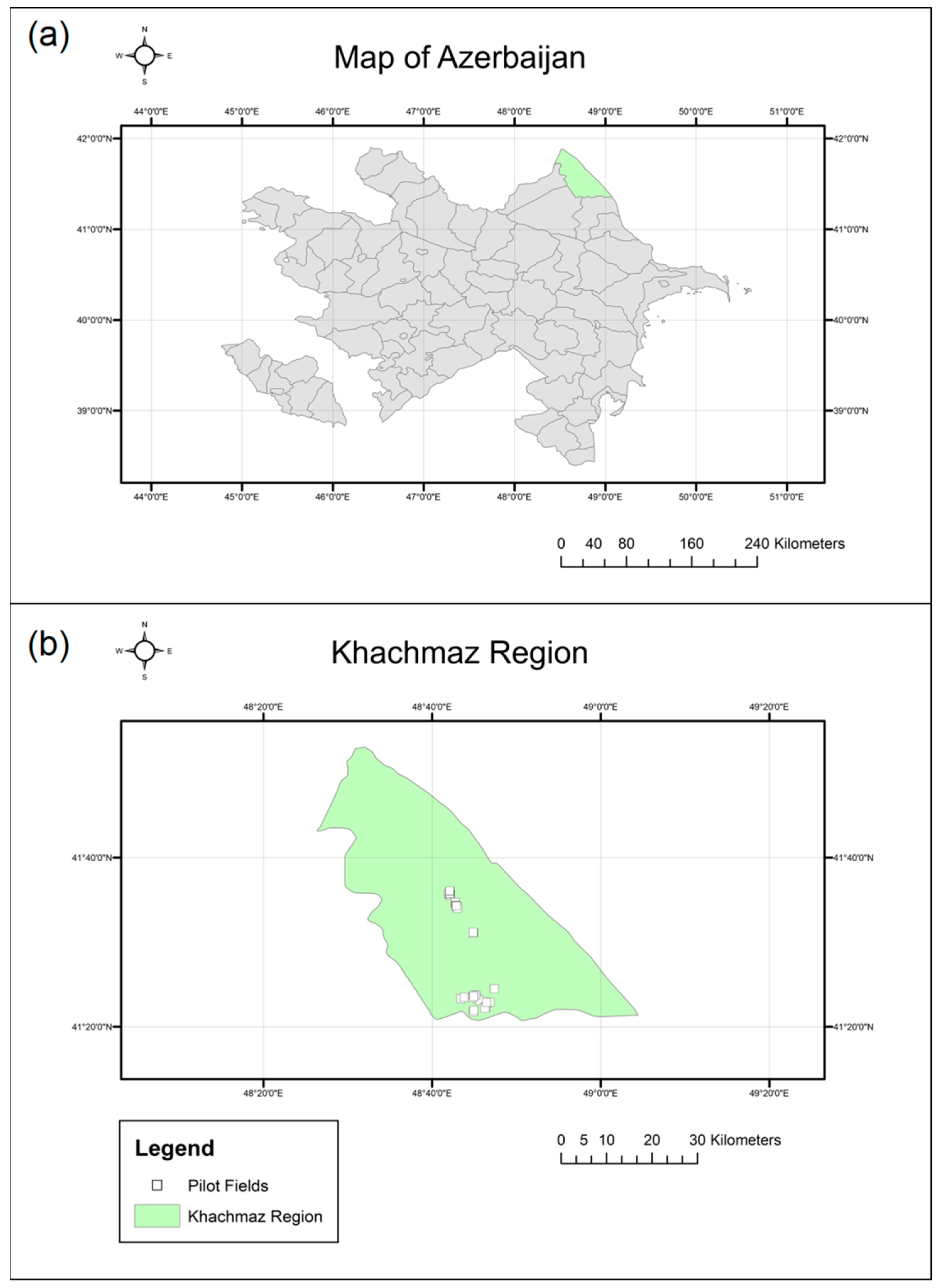
The study took place in the Khachmaz region of Azerbaijan, where 34 processing tomato fields with a total area of 128 ha (±SD = 5.75 ha) were selected as pilot fields for this study (extent of 41°21′40.2″ N 48°41′51.8″ E: 41°36′07.8″ N 48°47′24.8″). The planting date of the pilot fields ranged between the end of May and the beginning of June 2021, while harvesting was completed in all fields at the beginning of September. All pilot fields were irrigated and planted in rows with an average row spacing of 0.6–0.8 m, which corresponds to the extensive cropping system commonly used in the region. In addition, all fields were located in flat areas with a maximum slope of 10° within each field. The area of the study region is shown in Figure 1.

2.2. Data Collection and Pre-Processing

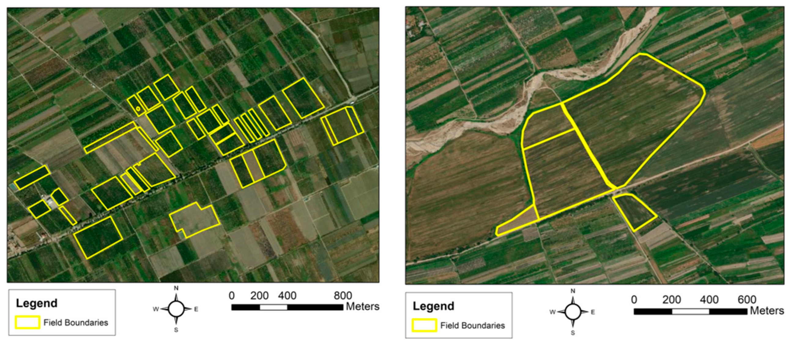
First, the pilot fields were digitised using topographic field data collected by agronomists of the Ministry of Agriculture (MOA) of the Republic of Azerbaijan in their respective regions using portable positioning systems in May 2021. These field measurements and the polygon boundary files generated were then checked and possibly fine-tuned using RGB components created from Azersky satellite imagery (SPOT-7) from the same period. An example of the vector layers of field boundaries acquired during these field measurements is presented in Figure 2.

The remote sensing data used in this study are 10 × 10 m² resolution multispectral images obtained from the Multi-Spectral Imager (MSI) sensor of ESA’s Sentinel-2 satellite platforms. The atmospherically corrected images (Level-2A, providing Bottom of Atmosphere reflectance values) from the Sentinel-2A satellite in cartographic geometry (UTM/WGS84 projection) were downloaded from the official Copernicus Open Access Hub (scihub.copernicus.eu, accessed on 30 September 2021). Since Khachmaz was heavily clouded throughout June, the first image mosaic that could be used was taken in early July (2021). In the event that heavy cloud cover occurred and the experimental fields of interest were not visible, the next available set of images was used instead. Satellite imagery data was collected at 10-day intervals, except for the first two measurements when heavy cloud cover over the study area required an increase in the interval to ensure the validity of the data. It was decided that the interval between two consecutive image captures should not be shorter than 10 days because (1) the field visits were necessary for the purposes of the project and had to be carried out in a timely manner and (2) no major fluctuations were to be expected at such short intervals.

For each data collection date, a total of four (4) images were downloaded to adequately cover the entire study area. The first step of data pre-processing involved the mosaicing of the individual images from each data collection date into orthoimages of the entire study area, using ArcGIS software (Environmental Systems Research Institute, Redlands, CA, USA). Once the total number of images was determined, an additional filtering step was applied to all regional images to ensure that each generated mosaic consisted exclusively of high-quality and cloud-free data from the pilot fields. This process was only carried out on the area covered by the vector layer containing the pilot fields, as an overall low cloud cover index for an image does not necessarily guarantee the visibility of the pilot fields and vice versa. In the event that high cloud cover occurred and the pilot fields were not visible, the next available set of images was used instead. The generated data cube consisted of five (5) cloud-free regional raster orthomosaics sampled at 10 × 10 m² resolution.

The next step, which spanned the entire cropping season, was to use each generated multispectral orthomosaic of the Khachmaz region to create plant vigour variability maps for the study fields. For this study, NDVI [24] was selected as the main vegetation index because of its ability to distinguish vigour patterns of foliage plants, its popularity in research, and its ease of replication for future implementations. Moreover, five additional widely used VIs, namely the Weighted Difference Vegetation Index (WDVI), Green Normalised Difference Vegetation (GNDVI), Soil-Adjusted Vegetation Index (SAVI), Modified Soil-Adjusted Vegetation Index (MSAVI) and Perpendicular Vegetation Index (PVI) were also used to assess their ability to describe crop status throughout the season and, naturally, the final yield. To this end, the VI orthomaps of the entire area were created by iterating the VI formulas over all satellite image pixels using the Raster Calculator tool of ArcGIS, resulting in the VI orthomaps of the study area. The Vis used in the present study and their respective equations are presented below (

Table 1. The selected Vis used in this study and their respective spectral equations.

Index	Equation	Reference
NDVI	$\frac{\left(\mathrm{NIR} – \mathrm{RED}\right)}{\left(\mathrm{NIR} + \mathrm{RED}\right)}$	[24]
GNDVI	$\frac{\left(\mathrm{NIR} – \mathrm{GREEN}\right)}{\left(\mathrm{NIR} + \mathrm{GREEN}\right)}$	[25]
WDVI	$\mathrm{NIR}-\mathrm{S}\ast \mathrm{RED}$ where: S is the slope of the soil line from a plot of red versus near infrared.	[26]
PVI	$\frac{\left(\mathrm{NIR} - \mathrm{a} \ast \mathrm{RED} - \mathrm{b}\right)}{\sqrt{\left(\mathrm{a}\Lambda 2 + 1\right) }}$ where a is the slope of the ground line and b is the ground line’s gradient.	[27]
MSAVI	$\frac{\left(\mathrm{NIR}-\mathrm{RED}) \ast \left(1 + \mathrm{L}\right)\right)}{\left(\mathrm{NIR} + \mathrm{RED} + \mathrm{L}\right)}$ $where: \mathrm{L}=\mathit{1}-\frac{\left(2 \ast s\ast \left(NIR-RED\right)\ast \left(NIR-s\ast RED\right)\right)}{\left(NIR+RED\right)}$ where s is the slope of the soil line from a plot of red versus near infrared brightness values	[28]
SAVI	$\frac{\left(\mathrm{NIR} - \mathrm{RED}\right)}{\left(\mathrm{NIR} + \mathrm{RED} + \mathrm{L}\right)} \ast \left(1+\mathrm{L}\right)$	[29]

):

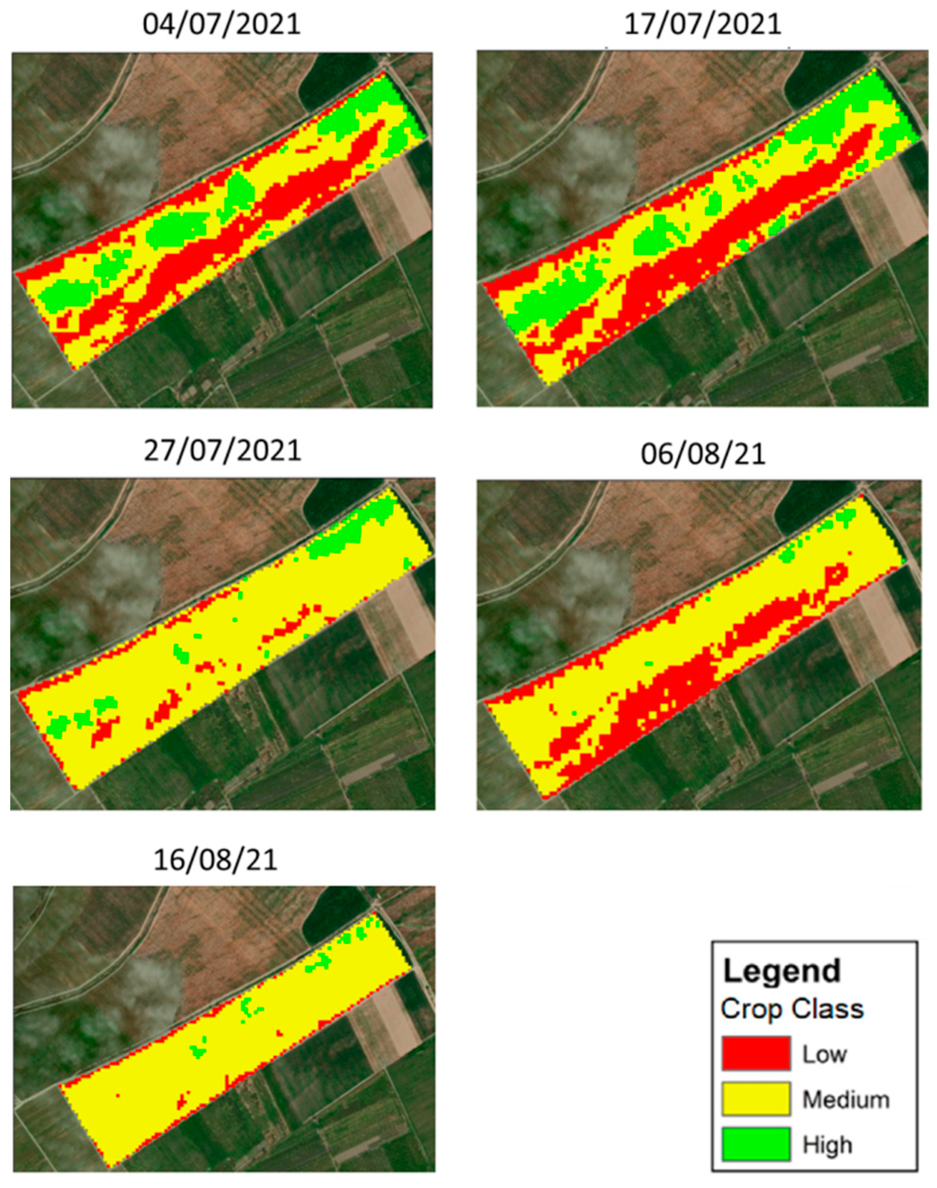
The VI maps served a dual purpose: (1) they are needed for the following steps of the methodology, as yield forecasts are essentially generated based on the cumulative values of each field throughout the season, but in addition (2) they can also serve as a valuable field management tool for farmers and agronomists during the cultivation season. These maps and the time series generated can provide information on which field segments need more attention and help to identify faulty areas easily and in a timely manner. Furthermore, as they were used to quantify the development of plant vigour in all pilot fields in near real time, they were also used to classify them based on their expected productivity. Therefore, once the original VI layers had been cropped using the field boundaries as a mask, for each selected date, all pixels in the new raster layer, were classified using a 3-class quantile classification to capture the overall picture of crop field performance in the region. This resulted in a new layer where each pilot field pixel was assigned a productivity class value based on the VI values recorded at the time of the last data collection, compared to all other pilot fields in the area. An example of the NDVI maps generated at a similar resolution to the original Sentinel-2 imagery (10 × 10 m²) for each data collection date for this season is shown in Figure 3.

Finally, for each field layer extracted using the pilot field boundaries as a “mask” on the regional orthomosaics, a mean VI value was extracted from each field. These values were finally integrated with their time interval (i.e., 10–13 days between each image) to produce the cumulative VI for each field in that season, or simply the area under the VI curve of each field.

2.3. In-Situ Data Collection Campaigns

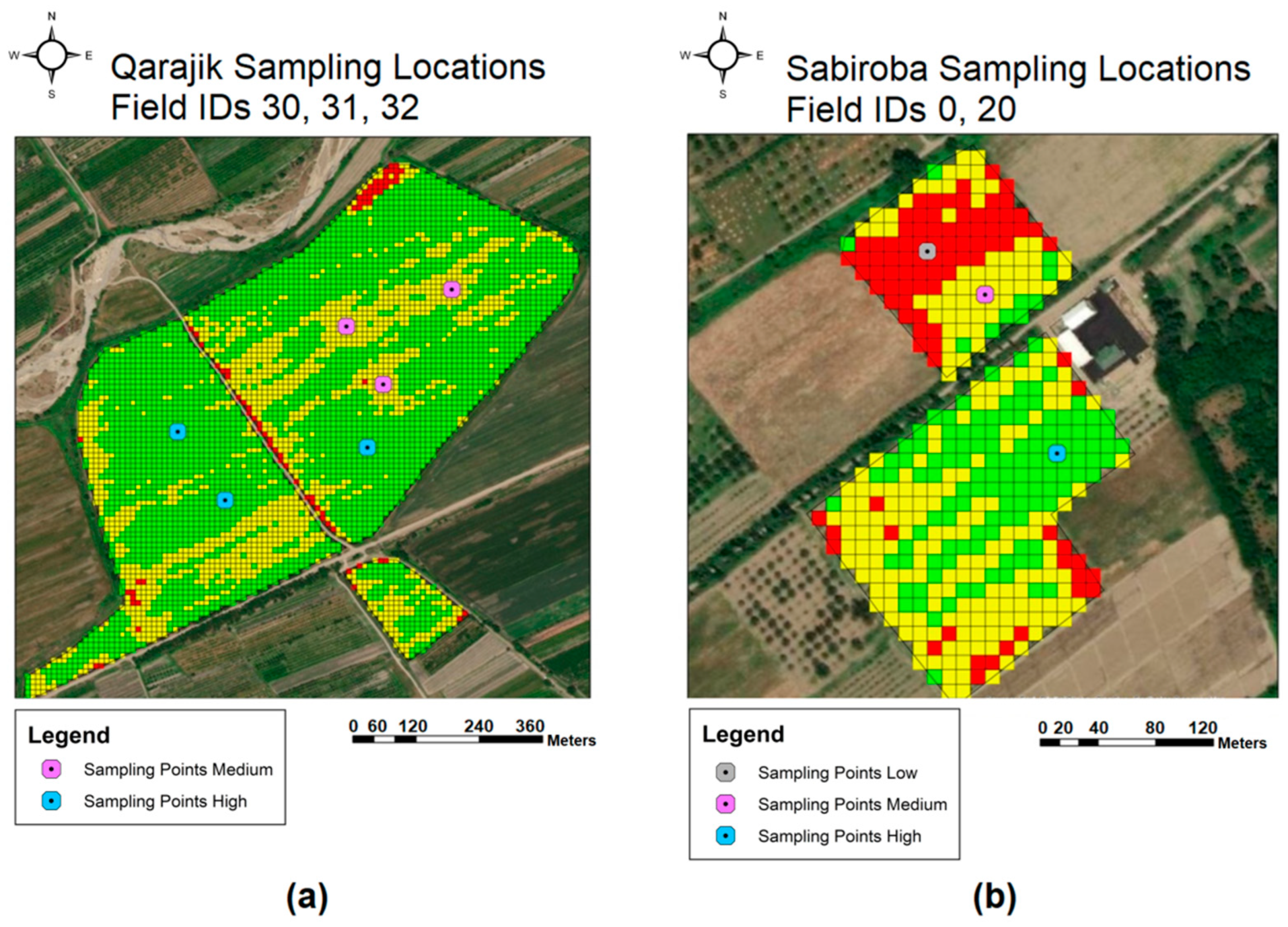
To evaluate the accuracy of the VI maps produced, field visits were made to Khachmaz district on selected dates towards the end of the cultivation season (early August) to collect in situ samples from targeted pilot fields productivity zones. Sampling sites were selected based on the most recently produced NDVI maps to verify the accuracy of the classification against actual data from the pilot fields. The soil sampling carried out on the selected processing tomato fields, which resulted in a total of 12 sampling visits, consisted of production measurements (yield weighting) in 1 m² cells, so that they can evaluate the validity of the productivity class assigned to that pixel. The sample locations were selected using a Python script that first identified the “purest” cells of each field, i.e., the pixels that were located in the centre of their respective zone and were exclusively and completely surrounded by pixels belonging to their class. A list of 36 selected sampling locations (12 sampling locations per class across all pilot fields) was then selected based on the number of classes present in each field and its total area. An example of two (2) selective sampling maps over the productivity quantile class layer (NDVI) with an integrated supporting 10 × 10 m² grid aligned with the grid of the satellite imagery to assist in locating the selected sampling locations are presented in Figure 4.

In addition to the targeted sampling at Khachmaz, field visits were conducted on several days throughout the cultivation season to assess zone classification and the overall accuracy of crop growth status maps. These visits, which were an additional validity check, were carried out in the presence of the farmers managing the respective fields or the agronomists in charge, and the main observations for each field visit were documented. Finally, at the end of the growing season, after the harvest was completed, the actual yields at field level were collected, expressed in t/ha. These data were needed to evaluate and update the crop-specific equation of the model, as it is expected to have the smallest possible error to these yield values. The actual yield of each pilot field was recorded directly by the farmers under the supervision of the MoA offices, and the respective total yield values were assigned to each pilot field. At the end of the season, a total of five (5) values for each of the six (6) VIs used and the recorded yield were assigned to each pilot field.

2.4. Statistical Analysis and Yield Estimation Equations

In this study, the first step of the selected yield forecasting method was to establish a baseline and a set of initial predictions by implementing a fitted equation following the approach of Kross et al., 2015 [30] using a biomass conversion function and a harvest index (HI). This linear approach is simple to implement and can be easily calibrated once actual yield data become available to update the model and significantly increase its accuracy.

The predictions naturally inherit the linearity of the implemented VIs and crop growth and are also divided into 3-class quantiles to determine which fields in the pilot area are likely to perform better than others. For the first run of the system, the NDVI was selected along with a biomass transfer factor of 1.9 and a HI of 0.6 for tomatoes based on existing literature [31,32]. Once the actual yield data had been collected, the linear equation values that best described the yield were determined. This resulted in the new updated crop-specific yield estimation model, which is of course much more accurate than the arbitrary approach based on the literature, as it was directly regressed on the data collected in this particular region. Furthermore, it has the potential to become even more robust with further similar iterations in upcoming years. For the statistical analysis of the correlations between the yield and VI data, the correlation coefficient estimates and regression analysis were performed using Statgraphics 16 (StatPoint Technologies Inc., Warrenton, VA, USA). Pearson’s correlation coefficient (r) and regression analysis (r²) were used to compare the spatial similarity between the different datasets by measuring the strength and direction of the linear relationship between the two variables. To determine the linear model that best describes the relationship between the VI data and the recorded yield, the “comparison of alternative models” function of Statgraphics was used. The linear regression model was selected based on the values of R squared, adjusted R squared, and Mean Absolute Error (MAE), since these are the most widely used evaluation metrics for regression models. Furthermore, an additional analysis was performed, to assess the cumulative capacity (data availability) of the satellite data, and how the cumulative VI approach performs when less data is used for the predictions.

3. Results

3.1. Descriptive Statistics

Before performing the correlation analysis, basic statistics were calculated to explore the data (

Table 2. The descriptive statistics of the NDVI mean values across all pilot fields during each data collection date.

Descr. Statistics	04_07mean	17_07mean	27_07mean	06_08mean	16_08mean
Average	0.299623	0.540446	0.535435	0.543585	0.493061
Standard deviation	0.110168	0.117534	0.0981507	0.0961387	0.082061
Coeff. of variation	36.77%	21.75%	18.33%	17.69%	16.64%
Minimum	0.146951	0.233852	0.251744	0.249079	0.283117
Maximum	0.600925	0.697956	0.712183	0.695276	0.639797
Range	0.453974	0.464104	0.460439	0.446196	0.35668

). The mean values of the individual NDVI values across all fields ranged from less than 0.15 at the beginning of the cropping season to over 0.71 in the middle of the season, showing high seasonal variability. A similar process was carried out for the different cumulative ranges, as well as for the recorded yield (

Table 3. The descriptive statistics of the recorded yield data and mean NDVI cumulative values across all cumulative ranges and pilot fields.

Descr. Statistics	Yield	Total [1–5]	[1–4]	[2–5]	[1–3]	[3–5]
Average	36.3618	21.4182	16.235	15.9577	10.8399	10.5783
Standard deviation	7.55938	3.72676	2.9828	2.73635	2.14434	1.74428
Coeff. of variation	20.79%	17.40%	18.37%	17.15%	19.78%	16.49%
Minimum	13.8	11.5837	8.92275	7.59308	6.41863	5.1651
Maximum	48.4	28.0466	21.3712	19.847	14.7301	13.3164
Range	34.6	16.4628	12.4485	12.254	8.31151	8.15133

). For the cumulative ranges, the variability of the values was much lower, which is another logical result since the NDVI values are integrated with the temporal interval (days between consecutive data collection dates on the X-axis), which by nature has much higher numerical values than the NDVI. Finally, a variable profile was also observed in the recorded yields, ranging from less than 14 t/ha to over 48 t/ha.

The descriptive statistics of the other five (5) VIs used in this study and their respective cumulative ranges are also presented in the following tables (

Table 4. The descriptive statistics of the WDVI mean values across all pilot fields during each data collection date.

Descr. Statistics	04_07mean	17_07mean	27_07mean	06_08mean	16_08mean
Average	0.0418	0.1844	0.1796	0.1766	0.1528
Standard deviation	0.0523	0.0683	0.0566	0.0537	0.0528
Coeff. of variation	1.2527	0.3705	0.3154	0.3040	0.3459
Minimum	−0.0267	0.0089	0.0248	0.0223	0.0372
Maximum	0.2025	0.2968	0.2854	0.2553	0.2400
Range	0.2293	0.2879	0.2605	0.2329	0.2028

,

Table 5. The descriptive statistics of the mean WDVI cumulative values across all cumulative ranges and pilot fields.

Descr. Statistics	Total [1–5]	[1–4]	[2–5]	[1–3]	[3–5]
Average	6.7195	5.0720	5.2490	3.2905	3.429
Standard deviation	2.1119	1.6853	1.5708	1.2062	0.9971
Coeff. of variation	0.3143	0.3322	0.2992	0.3665	0.2908
Minimum	1.3310	1.0334	0.7023	0.7975	0.5334
Maximum	10.3609	8.1072	7.5373	5.5693	4.8606
Range	9.0298	7.0737	6.8349	4.7717	4.3271

,

Table 6. The descriptive statistics of the GNDVI mean values across all pilot fields during each data collection date.

Descr. Statistics	04_07mean	17_07mean	27_07mean	06_08mean	16_08mean
Average	0.3233	0.5284	0.5167	0.5206	0.4764
Standard deviation	0.0846	0.0847	0.0700	0.0700	0.0598
Coeff. of variation	0.2617	0.1603	0.1355	0.1346	0.1256
Minimum	0.2026	0.2826	0.3050	0.3020	0.3106
Maximum	0.5545	0.6266	0.6201	0.6281	0.5902
Range	0.3519	0.3440	0.3150	0.3260	0.2795

,

Table 7. The descriptive statistics of the mean GNDVI cumulative values across all cumulative ranges and pilot fields.

Descr. Statistics	Total [1–5]	[1–4]	[2–5]	[1–3]	[3–5]
Average	20.9354	15.9504	15.398	10.7634	10.172
Standard deviation	2.7226	2.1732	1.9947	1.5701	1.2778
Coeff. of variation	0.13004	0.1362	0.1295	0.1458	0.1256
Minimum	13.3850	10.3213	9.0374	7.2859	6.0991
Maximum	25.8148	19.7229	18.2105	13.6316	12.1832
Range	12.4298	9.4016	9.1731	6.3456	6.0841

,

Table 8. The descriptive statistics of the SAVI mean values across all pilot fields during each data collection date.

Descr. Statistics	04_07mean	17_07mean	27_07mean	06_08mean	16_08mean
Average	0.1817	0.3747	0.3691	0.3664	0.3331
Standard deviation	0.0734	0.0889	0.0737	0.0718	0.0716
Coeff. of variation	0.4041	0.2372	0.1998	0.1960	0.2150
Minimum	0.0822	0.1406	0.1628	0.1566	0.1726
Maximum	0.4011	0.5172	0.5008	0.4750	0.4492
Range	0.3189	0.3766	0.3380	0.3184	0.2765

,

Table 9. The descriptive statistics of the mean SAVI cumulative values across all cumulative ranges and pilot fields.

Descr. Statistics	Total [1–5]	[1–4]	[2–5]	[1–3]	[3–5]
Average	14.5127	11.0145	10.8957	7.3364	7.1763
Standard deviation	2.7799	2.2130	2.0705	1.5836	1.3245
Coeff. of variation	0.1915	0.2009	0.1900	0.2159	0.1846
Minimum	7.3247	5.6514	4.7881	4.0541	3.2706
Maximum	19.3880	15.0379	13.9590	10.3390	9.0491
Range	12.0633	9.3865	9.1710	6.2849	5.7784

,

Table 10. The descriptive statistics of the MSAVI mean values across all pilot fields during each data collection date.

Descr. Statistics	04_07mean	17_07mean	27_07mean	06_08mean	16_08mean
Average	0.1559	0.3380	0.3318	0.3275	0.2965
Standard deviation	0.0112	0.0146	0.0121	0.0118	0.0120
Coeff. of variation	0.0721	0.0431	0.0365	0.0359	0.0403
Minimum	0.0690	0.1205	0.1398	0.1335	0.1388
Maximum	0.3587	0.4795	0.4635	0.4297	0.4084
Range	0.2898	0.3589	0.3237	0.2962	0.2696

,

Table 11. The descriptive statistics of the mean MSAVI cumulative values across all cumulative ranges and pilot fields.

Descr. Statistics	Total [1–5]	[1–4]	[2–5]	[1–3]	[3–5]
Average	12.9750	9.8554	9.7647	6.5591	6.4160
Standard deviation	0.4535	0.3601	0.3393	0.2568	0.2173
Coeff. of variation	0.0350	0.0365	0.0348	0.0392	0.0339
Minimum	6.2918	4.8637	4.0958	3.4975	2.7943
Maximum	17.5778	13.6749	12.6808	9.4104	8.2036
Range	11.2860	8.8112	8.5849	5.9128	5.4093

,

Table 12. The descriptive statistics of the PVI mean values across all pilot fields during each data collection date.

Descr. Statistics	04_07mean	17_07mean	27_07mean	06_08mean	16_08mean
Average	0.0735	0.1639	0.1612	0.1568	0.1438
Standard deviation	0.0309	0.0415	0.0347	0.0332	0.0362
Coeff. of variation	0.4196	0.2532	0.2150	0.2120	0.2520
Minimum	0.0325	0.0582	0.0673	0.0634	0.0592
Maximum	0.1698	0.2310	0.2259	0.2011	0.1956
Range	0.1373	0.1729	0.1586	0.1377	0.1363

and

Table 13. The descriptive statistics of the mean PVI cumulative values across all cumulative ranges and pilot fields.

Descr. Statistics	Total [1–5]	[1–4]	[2–5]	[1–3]	[3–5]
Average	6.2609	4.7581	4.7177	3.1683	3.0925
Standard deviation	1.2855	1.0156	0.9712	0.7226	0.6235
Coeff. of variation	0.2053	0.2134	0.2059	0.2281	0.2016
Minimum	3.0183	2.3389	1.9608	1.6850	1.3333
Maximum	8.3238	6.4995	6.1028	4.4879	4.0000
Range	5.3055	4.1606	4.1420	2.8029	2.6667

). As can be observed, most VIs follow a similar temporal pattern during the growing season and value distribution as the NDVI. They show their lowest values at the beginning of the growing season (04_07), followed by the highest values on the second data collection date (17_07), and then remain stable for the rest of the season. For the cumulative ranges, as the VI values are integrated into the temporal axis, VIs with inherently lower numerical values naturally show lower variability in their cumulative values. This is due to their “in-season” variability being normalised, something that can be easily observed in the case of PVI and GDVI, the two indices that have the lowest numerical values compared to the other indices.

3.2. Accuracy of Crop Growth Status Maps

In the last phase of the processing tomato cultivation season (mid-August), the data from the targeted in situ sampling expeditions were analysed and correlated with the individual NDVI quantile values of each sampled cell. This process was repeated for the maximum cumulative values that were available at that time (since the fifth and final set of Sentinel-2 images used in this study was not digested and thus not analysed at the time of the sampling campaigns). As the results of the analysis show, the Sentinel-2 images were good at assessing field productivity in near real-time. The correlation between quantile classification and recorded sample yield was high, especially for the maximum cumulative NDVI range at the time of measurement. The correlation between the productivity class assigned to the targeted sample points and their respective in situ yield samples, as well as red-only tomatoes harvested, is shown in

Table 14. The Pearson correlation values between the quantile classification of the NDVI data and the ground truth samples collected in early August.

Correlated Data	Correlation with Total Yield	Correlation with Red Tomatoes
Cumulative [1–4]	0.8586	0.9226
4th Measurement (06 August 2021)	0.7969	0.7627
3rd Measurement (27 July 2021)	0.7548	0.7597
2nd Measurement (17 July 21)	0.7471	0.7582
1st Measurement (04 July 2021)	0.1553	0.4483

.

3.3. Yield Estimation Models Calibration

The correlation values between VI data of a single date and the final yield across all fields are presented in

Table 15. The Pearson correlation coefficient between the single-date mean VI values and the recorded yield across all pilot fields.

VI	04_07	17_07	27_07	06_08	16_08
NDVI	0.438	0.840	0.809	0.809	0.739
WDVI	0.415	0.863	0.797	0.787	0.679
GNDVI	0.428	0.867	0.833	0.806	0.784
MSAVI	0.392	0.863	0.796	0.782	0.65
SAVI	0.397	0.864	0.804	0.788	0.661
PVI	0.376	0.862	0.786	0.764	0.621

and Figure 5. The regressions of the VI data at the single date with the highest correlation with yield are presented in

Table 16. The regression models that best describe yield (expressed in t/ha) through VI data for the selected date (17_07) along with their adjusted R-Squared and MAE values (All VIs presented significant correlations at the p < 0.05 level).

VI (17_07)	Regression Model	Adj. R2 (%)	MAE	p-Value
NDVI	Yield = 7.15 + 54.06 ∗ NDVI	69.7	3.05	<10−3
GNDVI	Yield = −4.52 + 77.36 ∗ GNDVI	74.4	2.84	<10−3
PVI	Yield = 10.61 + 157.14 ∗ PVI	73.6	2.98	<10−3
SAVI	Yield = 8.85 + 73.43 ∗ SAVI	73.8	2.92	<10−3
MSAVI	Yield = 10.43 + 76.74 ∗ MSAVI	73.7	2.93	<10−3
WDVI	Yield = 18.76 + 95.44 ∗ WDVI	73.7	2.93	<10−3

, showing the linear models that best fit the dataset created. The yield estimated by the equations of Table 16 is measured in tonnes per hectare (t/ha). The adjusted r² of the NDVI datasets, ranged from 0.166 to 0.697, with the lowest regression values recorded for the first measurement of the season and the highest for the second measurement. Similarly, the lowest and highest correlation values (for the same dates), were 0.438 and 0.840, respectively. The date with the highest correlation between yield and single-date VI data was 17_07 and was thus selected for separate regression analysis for all VIs (Figure 6).

A similar approach was used to evaluate the correlation between the cumulative data of all implemented VIs and the recorded yield, and the cumulative method consistently performed better than the single dates across all VIs (

Table 17. The Pearson correlation coefficient between the different cumulative VI ranges and the recorded yield across all pilot fields.

VI	Total [1–5]	[1–4]	[2–5]	[1–3]	[3–5]
NDVI	0.892	0.882	0.866	0.861	0.847
WDVI	0.887	0.879	0.858	0.866	0.830
GNDVI	0.905	0.896	0.877	0.874	0.854
MSAVI	0.884	0.877	0.855	0.863	0.824
SAVI	0.888	0.881	0.860	0.865	0.830
PVI	0.876	0.873	0.842	0.862	0.806

). In addition, as more data became available to the model (higher cumulative ranges), its performance generally increased. The highest accuracy was observed for the maximum cumulative capacity of all five (5) available data collection dates for all VIs, with a correlation of 0.892 and an r² of 0.789 for NDVI. The best cumulative VI was GNDVI, which achieved a correlation of 0.905 with final yield at its maximum cumulative range. The detailed results of the correlations for the other VIs are presented in Figure 7, while the regression models appear in

Table 18. The regression models that best describe yield (expressed in t/ha) through VI data for the maximum cumulative range [1–5], along with their adjusted R-Squared and MAE values (All VIs presented significant correlations at the p < 0.05 level).

VIs	Regression Model	adj. R2 (%)	MAE	p-Value
NDVI	Yield = −2.39 + 1.81 ∗ Cum. NDVI [1–5]	78.9	2.23	<10−3
GNDVI	Yield = −16.23 + 2.51 ∗ Cum. GNDVI [1–5]	81.3	2.10	<10−3
PVI	Yield = 4.11 + 5.15 ∗ Cum. PVI [1–5]	76.0	2.56	<10−3
SAVI	Yield = 1.32 + 2.42 ∗ Cum. SAVI [1–5]	78.2	2.36	<10−3
MSAVI	Yield = 3.60I + 2.53 ∗ Cum. MSAVI [1–5]	77.4	2.42	<10−3
WDVI	Yield = 15.03 + 3.17 ∗ Cum. WDVI [1–5]	78.0	2.35	<10−3

and Figure 8, with yield expressed in tonnes per hectare (t/ha). Finally, a regression of all the different cumulative ranges of NDVI and yield was performed, with all the regression models presented in Figure 9.

3.4. Regional—National Upscale

Finally, the predictions of the pilot fields were scaled-up to larger administrative units, namely regions (economic districts) or even the whole country. Knowing the total number of hectares of crops grown in a given region, the average prediction values can be used for larger projections. Essentially, this projection approach starts from the known fields and uses their projections to roughly estimate production at regional and national levels. This method is common for such projections and is used by many national organisations and public agencies (such as FAO), which collect and use 10–15% of the total cultivated area per crop for each region, to calculate production and yield metrics for larger units. In these applications the Khachmaz were scaled up and compared with the latest statistical values to assess their accuracy. In our implementation we selected the maximum cumulative range model of NDVI (as the main index of our study), and the initial yield predictions were made at a field level, similar to the yield regression strategy used to create the model. The results of the regional and national level predictions for each crop are presented in

Table 19. The projections on a regional and national level, using the most recent statistic data reports (source: stat.gov.az).

Seasonal Projection	Total ha Cultivated	Tons Produced	Prediction (36.36 t/ha)	Error
Khachmaz	2015	65,531	73,268	11.8%
Republic of Azerbaijan	19,371	774,877	704,363	9.1%

. The upscaled predictions of the system performed very well, with an error of 11.8% for tomato in Khachmaz district this year. Even for larger scales, such as at a national level, the models maintain their high accuracy, achieving an error of only 9.1% using the most recent data from MoA.

4. Discussion

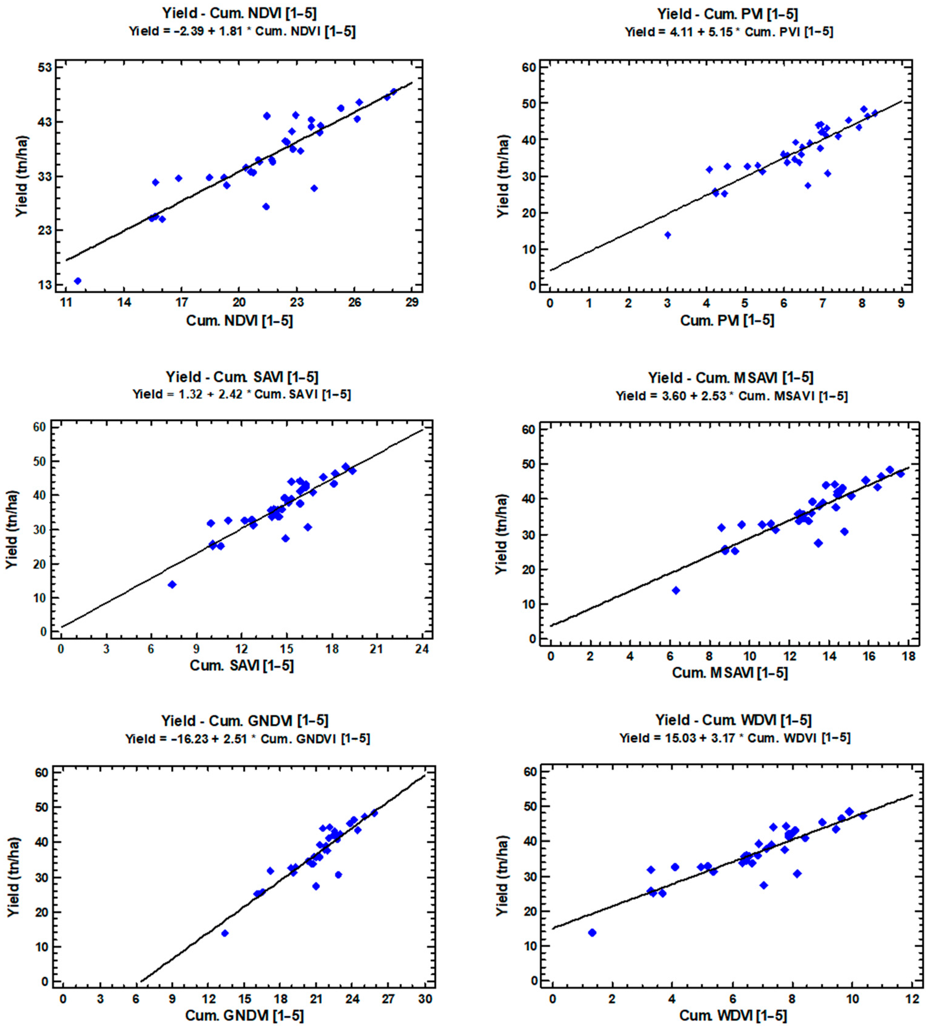
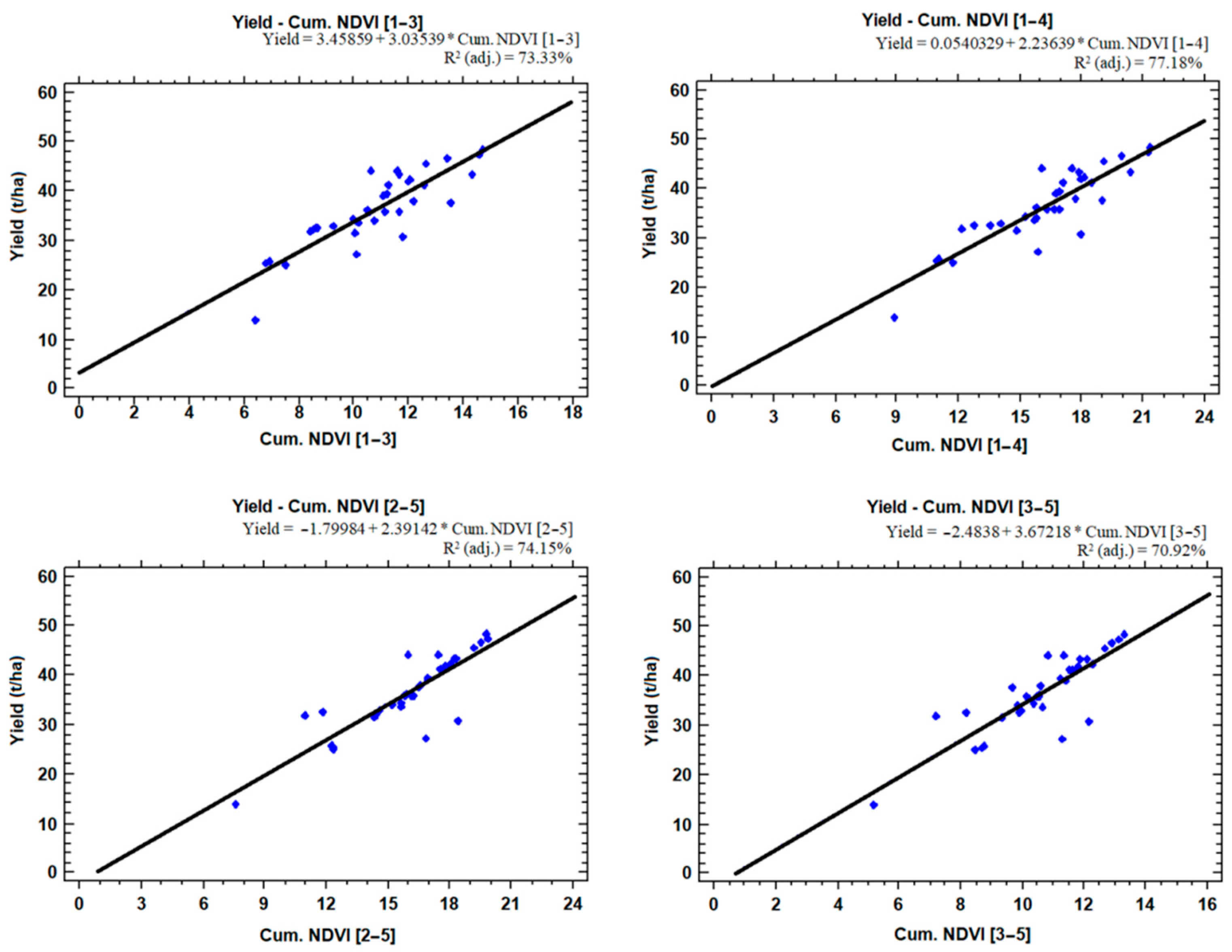
The results show that, across all of the experiments, the predictive capabilities of Sentinel-2 derived VI data are satisfactory. Specifically for NDVI, the performance of all cumulative NDVI models, regardless of cumulative range, was consistently above 0.84 correlations with the final recorded yield in all experimental fields in the Khachmaz region. The best performance for all VIs used in this study was obtained with the maximum cumulative range [1–5], which corresponds to the maximum data availability. The same pattern of “more data used, higher accuracy” was also found for the shorter cumulative ranges, as [1–4] and [2–5] outperformed [1–3] and [3–5] for most VIs. However, even the lower end of cumulative ranges achieved solid performances, considering the inherent limitations of only using three (3) images as predictive inputs.

The VI that demonstrated the highest performance in the maximum cumulative range was GNDVI, with a correlation of over 90% with final yield, followed by NDVI with a correlation of over 89%. SAVI, MSAVI and WDVI all demonstrated similar results in maximum cumulative capacity, while the lowest correlation was observed with PVI. This was also the case across all cumulative ranges, with PVI consistently demonstrating the lowest correlation with yield, while also exhibiting the lowest correlation value across all VIs, for all single dates and cumulative ranges, barely exceeding 80% for the [3–5] range and 37% at the 1st measurement.

For the correlation between single dates and the final yield, poor prediction capability of NDVI and all VIs was generally observed at very early crop growth stages, when vegetation is sparse and bare soil covers a significant portion of the fields’ total area. Moreover, the 1st measurement is the one exhibiting the highest variation (36.77%). This variability is to be expected in plants with variable ground cover at different growth stages, since in the early growth stages most of the satellite sampling grids are bare soil. The percentage of ground cover increases towards the middle of the season when tomato plants reach their maximum vigour before they start transferring sugars to their fruits. However, it cannot be assumed that this process of canopy development is homogeneous and synchronous in several fields. The different planting dates are a logical explanation for the different vegetation cover during the planting period.

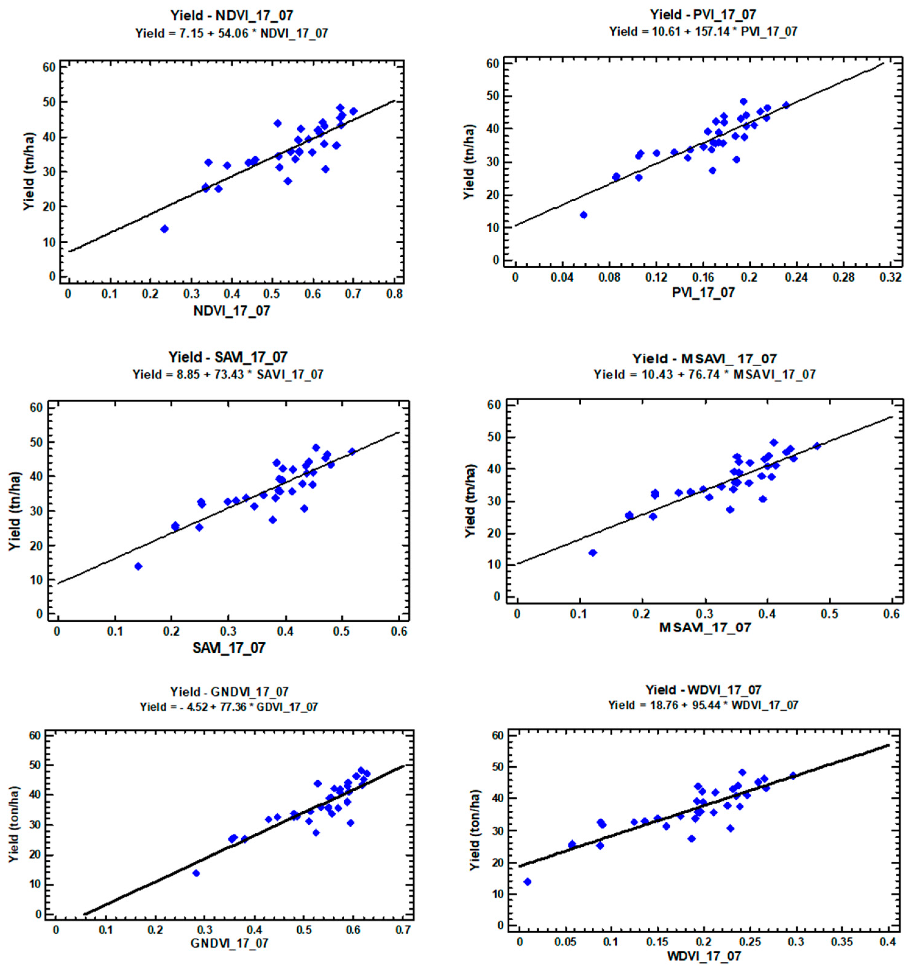
On the other hand, the primary canopy development stages (2nd measurement, 17_07) appeared to be strongly correlated with the final yield, possibly indicating a critical stage when processing tomato crops undergo changes that can be distinguishable through Sentinel-2 derived data. These results indicate a potential robust relationship between processing tomato yield and remote sensing VI datasets, displaying satisfactory linear correlation coefficients, and provide new insights into the monitoring of processing tomato fields at the Sentinel-2 resolution scale of 10 × 10 m². The fact that the differences between the minimum and maximum yield values are 34.6 t/ha show that there is room for improvement through more efficient field management strategies and decisions.

Another interesting comparison can be made between SAVI and MSAVI, the latter being essentially the modified version of the former, to mitigate the effect of bare soil on its values. To this end, some degree of variation would logically be expected, especially in early development stages. This was confirmed by our results, with the MSAVI generally being a less variable index and the SAVI having 6 times higher Standard Deviation across the growing season. Despite the fact that the MSAVI was one of the least variable indices, while the SAVI was one of the most variable ones, both had very similar performance values in terms of correlation with final yield, for single dates and for different cumulative ranges.

Regarding the homogeneity of the mean cumulative NDVI data, the range of values within a single date is minimised towards the end of the season (5th measurement, 16_08), after remaining fairly constant during most of the cultivation season. Interestingly, the highest variability between the different cumulative ranges is encountered in the maximum cumulative range (all 5 dates), which had twice as much heterogeneity compared to the two lowest cumulative ranges ([1–3] and [3–5]). The method used in the paper initially extracted the mean NDVI values of each field from each measurement date, and then used to calculate the cumulative values. The reason this method was followed, is because yield measurements would be collected in a field-level, as sub-field yield mapping would not be sustainable when developing a similar model with multiple fields in this region as input data. In future research, however, it would be interesting to experiment with a higher resolution yield sampling approach, even in a lower number of fields, to assess the capacity and compare the results with cumulative NDVI in specific field segments instead of the entire field.

Finally, an interesting finding regarding the upscaling of the predictions at regional and national levels was that the prediction for the Khachmaz region was overestimated by the maximum range ([1–5]) cumulative model, while the national forecast was underestimated. Considering that Khachmaz is one of the largest tomato producers in the country, this observation would normally indicate that several problems occurred in 2021 significantly affected the production of the region. In fact, during the seasonal field visits across the experimental region, several farmers had expressed concerns related to issues with irrigation, especially during early July, when the majority of the fields demonstrated peak vigour (seasonal NDVI maxima). Moreover, shortly after this period, the NDVI values started decreasing, although this is not necessarily related to symptoms due to water stress, as it is common for crops with high sugar and water content fruits to exhibit this behaviour during late growth stages [17,22].

5. Conclusions

In this study, Sentinel-2 satellite imagery was used to monitor crop status and develop a yield prediction model for processing tomato fields. For this purpose, six (6) VIs were calculated for five different dates based on atmospherically corrected Sentinel-2 images. The results demonstrated the high potential of Sentinel-2 images to monitor the fields’ vigour and predict the tomato yield at a territorial (regional) scale. This outcome is encouraging in the view of developing a wide-scale monitoring system, especially relying on the Sentinel-2 mission, allowing free access to data with high spatial and temporal resolution from most regions of the world.

In general, the results of the analysis show a satisfactory correlation of VIs with processing tomato yield at certain growth stages and give the impetus for further research over a longer period and on a larger scale. Agronomists and farmers can use this valuable knowledge as an operational tool to make precise spatially distributed interventions to improve the field productivity in a timely manner. In a future study, the developed system (developed as part of the activities of the EU-funded “Integrated Regional Development of Azerbaijan (IRDA)” Programme) will continue its activities this year and expand the developed models by both replicating more processing tomato field trials, but also expanding to more crops of interest.

References

1. Kerimov, N. Business Outlook in Azerbaijan; Deloitte: London, UK, 2021. [Google Scholar]
2. Valiyev, A.; Rustamov, F.V.O.; Huseynova, R.A.; Orujova, M.S.; Musayeva, S.N. The Digitalization Effectiveness as an Innovative Factor Development of the Agriculture in Azerbaijan. JEECAR 2022, 9, 194–205. [Google Scholar] [CrossRef]
3. Kaplan, G.; Fine, L.; Lukyanov, V.; Manivasagam, V.S.; Malachy, N.; Tanny, J.; Rozenstein, O. Estimating Processing-tomato Water Consumption, Leaf Area Index, and Height Using Sentinel-2 and VENµS Imagery. Remote Sens. 2021, 13, 1046. [Google Scholar] [CrossRef]
4. Ihuoma, S.O.; Madramootoo, C.A.; Kalacska, M. Integration of Satellite Imagery and in Situ Soil Moisture Data for Estimating Irrigation Water Requirements. Int. J. Appl. Earth Obs. Geoinf. 2021, 102, 102396. [Google Scholar] [CrossRef]
5. Chiesi, M.; Angeli, L.; Battista, P.; Fibbi, L.; Rapi, B.; Gozzini, B.; Maselli, F. Monitoring and Analysis of Crop Irrigation Dynamics in Central Italy through the Use of MODIS NDVI Data. Eur. J. Remote Sens. 2022, 55, 23–36. [Google Scholar] [CrossRef]
6. Campillo, C.; Carrasco, J.; Millán, S.; Martinez, L.; Prieto, M.H. Use of Sensors and Spatial Variability to Fertilization Management in Processing Tomato. In Proceedings of the XV International Symposium on Processing Tomato 1233, Athens, Greece, 11–15 June 2018; pp. 73–82. [Google Scholar]
7. Bhattarai, G.P.; Schmid, R.B.; McCornack, B.P. Remote Sensing Data to Detect Hessian Fly Infestation in Commercial Wheat Fields. Sci. Rep. 2019, 9, 6109. [Google Scholar] [CrossRef] [PubMed]
8. Chemura, A.; Mutanga, O.; Dube, T. Separability of Coffee Leaf Rust Infection Levels with Machine Learning Methods at Sentinel-2 MSI Spectral Resolutions. Precis. Agric. 2017, 18, 859–881. [Google Scholar] [CrossRef]
9. Atzberger, C. Advances in Remote Sensing of Agriculture: Context Description, Existing Operational Monitoring Systems and Major Information Needs. Remote Sens. 2013, 5, 949–981. [Google Scholar] [CrossRef]
10. Segarra, J.; Buchaillot, M.L.; Araus, J.L.; Kefauver, S.C. Remote Sensing for Precision Agriculture: Sentinel-2 Improved Features and Applications. Agronomy 2020, 10, 641. [Google Scholar] [CrossRef]
11. Jensen, J.R. Remote Sensing of the Environment an Earth Resource Perspective; Prentice Hall: Upper Saddle River, NJ, USA, 2000. [Google Scholar]
12. Gianquinto, G.; Orsini, F.; Fecondini, M.; Mezzetti, M.; Sambo, P.; Bona, S. A Methodological Approach for Defining Spectral Indices for Assessing Tomato Nitrogen Status and Yield. Eur. J. Agron. 2011, 35, 135–143. [Google Scholar] [CrossRef]
13. Zarco-Tejada, P.J.; González-Dugo, V.; Berni, J.A. Fluorescence, Temperature and Narrow-Band Indices Acquired from a UAV Platform for Water Stress Detection Using a Micro-Hyperspectral Imager and a Thermal Camera. Remote Sens. Environ. 2012, 117, 322–337. [Google Scholar] [CrossRef]
14. Padilla, F.M.; Peña-Fleitas, M.T.; Gallardo, M.; Thompson, R.B. Threshold Values of Canopy Reflectance Indices and Chlorophyll Meter Readings for Optimal Nitrogen Nutrition of Tomato. Ann. Appl. Biol. 2015, 166, 271–285. [Google Scholar] [CrossRef]
15. Fortes, R.; Prieto, M.H.; Terrón, J.M.; Blanco, J.; Millan, S.; Campillo, C. Using Apparent Electric Conductivity and NDVI Measurements for Yield Estimation of Processing-tomato Crop. Trans. ASABE 2014, 57, 827–835. [Google Scholar]
16. Fortes Gallego, R.; Prieto Losada, M.D.H.; García Martín, A.; Córdoba Pérez, A.; Martínez, L.; Campillo Torres, C. Using NDVI and Guided Sampling to Develop Yield Prediction Maps of Processing-tomato Crop. Span. J. Agric. Res. 2015, 13, e0204. [Google Scholar]
17. Anastasiou, E.; Balafoutis, A.; Darra, N.; Psiroukis, V.; Biniari, A.; Xanthopoulos, G.; Fountas, S. Satellite and Proximal Sensing to Estimate the Yield and Quality of Table Grapes. Agriculture 2018, 8, 94. [Google Scholar] [CrossRef]
18. Yang, P.; Tan, G.X.; Zha, Y.; Shibasaki, R. Integrating Remotely Sensed Data with an Ecosystem Model to Estimate Crop Yield in North China. In Proceedings of the XXth ISPRS Congress Proceedings Commission VII, WG VII/2, Istanbul, Turkey, 13–23 July 2004; pp. 150–156. [Google Scholar]
19. Tucker, C.J.; Holben, B.N.; Elgin, J.H., Jr.; Mcmurtrey, J.E., III. Relationship of Spectral Data to Grain Yield Variation: Remote Sensing of Winter Wheat Field. Photogramm. Eng. Remote Sens. 1980, 46, 19800051130. [Google Scholar]
20. Fieuzal, R.; Bustillo, V.; Collado, D.; Dedieu, G. Combined Use of Multi-Temporal Landsat-8 and Sentinel-2 Images for Wheat Yield Estimates at the Intra-Plot Spatial Scale. Agronomy 2020, 10, 327. [Google Scholar] [CrossRef]
21. Toscano, P.; Castrignanò, A.; Di Gennaro, S.F.; Vonella, A.V.; Ventrella, D.; Matese, A. A Precision Agriculture Approach for Durum Wheat Yield Assessment Using Remote Sensing Data and Yield Mapping. Agronomy 2019, 9, 437. [Google Scholar] [CrossRef]
22. Darra, N.; Psomiadis, E.; Kasimati, A.; Anastasiou, A.; Anastasiou, E.; Fountas, S. Remote and Proximal Sensing-Derived Spectral Indices and Biophysical Variables for Spatial Variation Determination in Vineyards. Agronomy 2021, 11, 741. [Google Scholar] [CrossRef]
23. Koller, M.; Upadhyaya, S.K. Prediction of Processing-tomato Yield Using a Crop Growth Model and Remotely Sensed Aerial Images. Trans. ASAE 2005, 48, 2335–2341. [Google Scholar] [CrossRef]
24. Rouse, J.W.; Haas, R.H.; Schell, J.A.; Deering, D.W. Monitoring Vegetation Systems in the Great Plains with ERTS. In Proceedings of the Third Earth Resources Technology Satellite-1 Symposium, NASA SP-351. Washington, DC, USA, 10–14 December 1974; pp. 301–317. [Google Scholar]
25. Gitelson, A.A.; Merzlyak, M.N. Remote sensing of chlorophyll concentration in higher plant leaves. Adv. Space Res. 1998, 22, 689–692. [Google Scholar] [CrossRef]
26. Clevers, J.G. Application of a weighted infrared-red vegetation index for estimating leaf area index by correcting for soil moisture. Remote Sens. Environ. 1989, 29, 25–37. [Google Scholar] [CrossRef]
27. Perry, C.R., Jr.; Lautenschlager, L.F. Functional equivalence of spectral vegetation indices. Remote Sens. Environ. 1984, 14, 169–182. [Google Scholar] [CrossRef]
28. Qi, J.; Chehbouni, A.; Huete, A.R.; Kerr, Y.H.; Sorooshian, S. A modified soil adjusted vegetation index. Remote Sens. Environ. 1994, 48, 119–126. [Google Scholar] [CrossRef]
29. Huete, A.R. A soil-adjusted vegetation index (SAVI). Remote Sens. Environ. 1988, 25, 295–309. [Google Scholar] [CrossRef]
30. Kross, A.; McNairn, H.; Lapen, D.; Sunohara, M.; Champagne, C. Assessment of RapidEye Vegetation Indices for Estimation of Leaf Area Index and Biomass in Corn and Soybean Crops. Int. J. Appl. Earth Obs. Geoinf. 2015, 34, 235–248. [Google Scholar] [CrossRef]
31. Gianfagna, T.J.; Logendra, L.; Durner, E.F.; Janes, H.W. Improving Tomato Harvest Index by Controlling Crop Height and Side Shoot Production. Life Support Biosph. Sci. 1998, 5, 255–261. [Google Scholar]
32. Shu, L.-Z.; Liu, R.; Min, W.; Wang, Y.; Hong-mei, Y.; Zhu, P.; Zhu, J. Regulation of Soil Water Threshold on Tomato Plant Growth and Fruit Quality under Alternate Partial Root-Zone Drip Irrigation. Agric. Water Manag. 2020, 238, 106200. [Google Scholar] [CrossRef]
Figure 1. The study area: (a) map of Azerbaijan and the location of the study area; (b) the distribution of the study fields in the study area.
Remotesensing 14 04202 g001
Figure 2. An example of the field boundaries’ layer, generated from topographical measurements in Khachmaz region, prior to the start of the cultivation season.
Remotesensing 14 04202 g002
Figure 3. Example of the NDVI maps generated throughout the cultivation season in the respective data collection dates for a single field, in quantile classification using all Khachmaz pilot fields.
Remotesensing 14 04202 g003
Figure 4. Two targeted sampling maps and the sampling location indicated by point vectors. The sampling locations took place in the (a) Qaracik Zeyid and (b) Sabiroba villages of Khachmaz, respectively.
Remotesensing 14 04202 g004
Figure 5. The correlation between single-date mean VI data and recorded yield, for all implemented VIs across all fields.
Remotesensing 14 04202 g005
Figure 6. The linear regression models that describe the relationship between the selected single-date (17_07) VI mean (field-level) values and the corresponding recorded yield (likewise for each field).
Remotesensing 14 04202 g006
Figure 7. The correlation between different cumulative ranges and recorded yield, for all implemented VIs.
Remotesensing 14 04202 g007
Figure 8. The linear regression model that describes the relationship between the total cumulative VI range values and the corresponding recorded yield across all pilot fields.
Remotesensing 14 04202 g008
Figure 9. The linear regression models that describe the relationship between the different selective cumulative NDVI range values and the corresponding recorded yield across all pilot fields.
Remotesensing 14 04202 g009