Article

A Polarization Stacking Method for Optimizing Time-Series Interferometric Phases of Distributed Scatterers

School of Geosciences and Info-Physics, Central South University, Changsha 410083, China
*
Author to whom correspondence should be addressed.
Remote Sens. 2022, 14(17), 4168; https://doi.org/10.3390/rs14174168
Submission received: 20 July 2022 / Revised: 12 August 2022 / Accepted: 17 August 2022 / Published: 25 August 2022
(This article belongs to the Special Issue Recent Progress and Applications on Multi-Dimensional SAR)

Abstract

:
For time-series interferometric phases optimization of distributed scatterers (DSs), the SqueeSAR technology used the phase linking (PL) to extract the equivalent single-master (ESM) interferometric phases from the multilooking time-series coherence matrix. The Cramer–Rao lower bound (CRLB) for the PL describes the highest achievable estimation accuracy of the ESM phases, which depends on the number of looks and the time-series coherence magnitude matrix. With the abundance of time-series polarimetric SAR data, many scholars have studied the coherence magnitude-based polarimetric optimization methods for optimizing the DS’s time-series interferometric phases, for example, the widely-used exhaustive search polarimetric optimization (ESPO) algorithm. However, the traditional polarimetric optimization methods select the boundary extremums of the coherence region (CR) as the optimized complex coherence, which is usually biased from the free-noise one. Currently, in the polarimetric InSAR (PolInSAR) technology, Shen et al. innovatively considered polarimetric information as statistical samples and proposed the total power (TP) coherency matrix construction method for increasing the number of looks and reducing the interferometric phase noise. Therefore, to optimize the time-series interferometric phases for DS, this paper proposes performing a polarization stacking and extending the PolInSAR TP construction to the time-series PolInSAR (TSPolInSAR) data configuration, called the time-series TP (TSTP) method. Simulated and real experiments prove that the new TSTP construction method has better performance and higher efficiency than the single polarimetric and the traditional ESPO algorithms.

1. Introduction

For the synthetic aperture radar (SAR) interferometry (InSAR) technology, the observed interferometric signal records the target scattering variance and the distance difference between two SAR acquisitions, corresponding to the decorrelation magnitude caused by the scatterers’ changes [1] and the interferometric phase of the deformation signal and atmospheric delay [2], respectively. However, the monitoring capability of the differential InSAR (DInSAR) technology is degraded by the decorrelation and the atmospheric delay. To overcome the aforementioned decorrelation limitation, many scholars have attempted to focus on the utilization of persistent scatterer (PS) and proposed a series of PS interferometry (PSI) technologies, for example, the permanent scatterer interferometry [3,4], the interferometric point target analysis (IPTA) [5], the PS pair (PSP) interferometry [6], and the Stanford Method for PS (StaMPS) [7,8]. To overcome the restriction that the PS is less present in the natural scene, the research focus of the time-series InSAR (TSInSAR) technologies has shifted to the distributed scatterer (DS)-based temporal analysis, for example, the small baseline subset (SBAS) technology [9,10,11], the coherent point technique (CPT) [12], the SqueeSAR technology [13], and the temporarily coherent point InSAR (TCP-InSAR) [14,15].
In contrast to PS with temporarily stable scattering behavior, DS normally contains a coherent sum of small and random scatterers that are susceptible to temporal-spatial decorrelation. As a state-of-the-art distributed scatterer interferometry (DSI) implementation, the SqueeSAR technology [13] proposed the space adaptive filtering with a two-sample Kolmogorov–Smirnov (KS) test and the phase triangulation algorithm (PTA) to effectively reduce the speckle noise and reconstruct the equivalent single-master (ESM) interferometric phases, respectively. Therefore, the time-series interferometric phases optimization of DS contains two key steps, including multi-temporal filtering (MTF) and phase linking (PL) [16]. (1) In terms of MTF, Jiang et al. constructed the confidence interval for each pixel according to the central limit theorem and proposed the fast statistically homogeneous pixel selection (FaSHPS) [17]. Dong et al. employed the likelihood ratio test (LRT) on the complex Wishart distributed covariance matrices to measure the similarity between two pixels [18]. (2) In terms of PL, Fornaro et al. proposed the eigenvalue decomposition (EVD)-based CAESAR method [19] to extract the dominant scattering mechanism; compared to the PTA, Ansari et al. achieved the maximum likelihood estimation (MLE) by EVD more efficiently, called the EMI method [20]. It has been demonstrated that the optimization performance of the PL algorithms can also be enhanced by the spatial coherence refinement, which could benefit from the bias removal and variance mitigation [21]. In addition, faced with the near-real-time (NRT) processing problem of the Big SAR data, Ansari et al. divided the time-series data into several small batches and proposed a sequential version of the PL estimator [22].
With the abundance of time-series polarimetric InSAR (PolInSAR) (TSPolInSAR) data, many scholars have studied the DS-oriented polarimetric optimizations to find an optimal polarimetric channel for the time-series interferometric phases optimization. Neumann et al. investigated two approaches for polarimetric optimization of multibaseline interferometric coherence [23]. Navarro-Sanchez and Lopez-Sanchez raised an exhaustive search polarimetric optimization (ESPO) algorithm for maximizing the averaged coherence magnitude [24] and applied it to deformation monitoring [25]. To alleviate the time-consuming problem in the ESPO method, Iglesias et al. put forward two new search modes for polarimetric optimization [26], including the Best and the suboptimum scattering mechanism (SOM) algorithms. To achieve a better tradeoff between the algorithm accuracy and the computation efficiency, Zhao and Mallorqui proposed the CMD-based Best method [27] by means of the combination of the coherency matrix decomposition (CMD) and the Best optimization. Wu et al. proposed a polarimetric optimization method based on the Signal-to-Noise Ratio (SNR) maximization [28], which requires a lower time cost than the ESPO algorithm. Zahra Sadeghi et al. used a temporal phase coherence (TPC)-based criterion to select the optimal polarimetric channel for each pixel [29], which could work well even in nonurban environments. Currently, in the PolInSAR technology, from the perspective of increasing the number of looks, Shen et al. considered polarimetric information as statistical samples innovatively and proposed the total power (TP) coherency matrix construction [30], which was also applied to optimize the PS candidates successfully [31].
Guarnieri and Tebaldini [32] have pointed out that the optimization performance of DS’s time-series interferometric phases is determined by the Cramer–Rao lower bound (CRLB) of the PL, which depends on the number of looks and the time-series coherence magnitude matrix. The traditional polarimetric optimization methods can increase the whole coherence magnitude level and further improve the reconstruction performance of the ESM interferometric phases. However, the polarimetric optimization methods usually select the boundary extremums of the coherence region (CR) as the optimized complex coherence, which is biased from the free-noise one in the case of the multilooking speckle noise, called the unstable statistical properties in this paper. Different from the coherence magnitude-based polarimetric optimization method, to better utilize the full polarimetric information to improve the time-series phase quality for DS, we perform a polarization stacking and extend the PolInSAR TP construction to the TSPolInSAR data configuration, called the time-series TP (TSTP) method. The research motivation based on the CRLB, the new method, and the proposed algorithm flow will be introduced in Section 2. In addition, Section 2 also gives the basic knowledge of TS(Pol)InSAR data generation, the multi-dimensional coherency matrix statistics, and the PL theory. Simulated and real experimental results and discussions over the following three polarimetric optimizations are seen in Section 3 and Section 4, respectively, including the single polarimetric, the ESPO, and the proposed TSTP methods. Conclusions are drawn in Section 5.

2. Method

2.1. TS(Pol)InSAR Data Generation

For PolSAR, a complex Pauli basis scattering vector can be used for describing full polarimetric information in the case of the reciprocal backscattering
k P o l = s H H + V V s H H V V 2 s H V T / 2
where s H H + V V = s H H + s V V , s H H V V = s H H s V V , s H V is a complex scattering signal from the horizontal transmitting and vertical receiving polarizations, and T denotes the matrix transpose.
For PolInSAR, a polarimetric interferometric scattering vector k P o l I n consists of master and slave complex Pauli basis scattering vectors k P o l 1 and k P o l 2 . The six-dimensional polarimetric interferometric (PolIn) coherency matrix is expressed as [33]
T P o l I n = k P o l I n k P o l I n H = T P o l 1 Ω Ω H T P o l 2 ,   k P o l I n = k P o l 1 k P o l 2
where H is complex conjugated transpose and · stands for multilooking average. T P o l and Ω are the polarimetric coherency and the interferometric cross-correlation matrices, respectively.
For any polarimetric channel ω , the complex interferometric coherence γ ω is generally denoted as [33]
γ ω = γ ω exp i ϕ ω = ω H Ω ω ω H T P o l 1 ω ω H T P o l 2 ω
The standard TS(Pol)InSAR data with N acquisitions consists of N(N − 1)/2 (polarimetric) interferometric pairs with different temporal-spatial baselines. For a polarimetric channel, the time-series interferometric (TSIn) coherency matrix represents the interferometric information between all acquisitions and can be obtained by averaging some spatial samples [13]
T T S I n = k T S I n k T S I n H ,   k T S I n = s 1 , , s N T
where T T S I n N × N and k T S I n are the time-series interferometric scattering vector of N images.

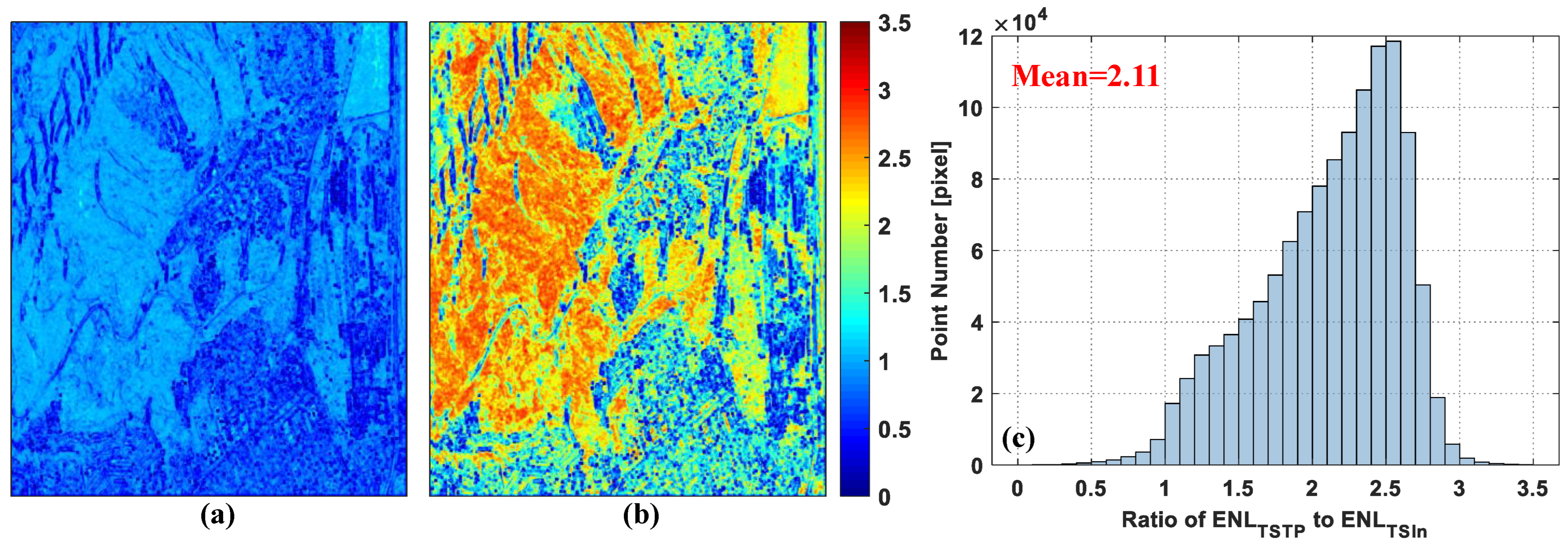
2.2. TS(Pol)InSAR Coherency Matrix Statistic and Equivalent Number of Looks (ENL) Estimation

TS(Pol)InSAR Coherency Matrix Statistic: The TS(Pol)InSAR coherency matrix is usually generated from the outer product of a multi-dimensional complex scattering vector, whose dimension increases with the increase of the temporal observation or the polarization channel. The q-dimensional single-look scattering vector k is denoted by [33]
k = s 1 s 2 s q T
Under the assumption that one resolution cell contains many elementary scatterers with fully developed speckle noise, k can be modeled following a multivariate complex Gaussian distribution with mean zero and covariance matrix Σ = E k k H , i.e., k N 0 , Σ [33], where E · denotes the mathematical expectation of the matrix k k H .
Usually, the multilooking processing needs to be used to reduce the speckle noise in the TS(Pol)InSAR coherency matrix. The resulting q-dimensional and n-look coherency matrix is obtained by averaging several independent single-look samples [34]:
T = 1 n i = 1 n k i k i H
Let A = n T , and the matrix A follows a complex Wishart distribution, i.e., A W q , n , Σ , whose probability distribution function (pdf) can be expressed as [34]
P q , n , Σ A = A n q exp Tr Σ 1 A π q ( q 1 ) / 2 Σ n j = 1 q Γ n j + 1
where Π denotes the product operation, Tr · represents the trace of the matrix, and Γ · is the gamma function. In addition, Σ and Σ 1 are the determinant and the inverse of the matrix Σ , respectively.
Equivalent Number of Looks (ENL) Estimation: The multilooking operator can effectively suppress the speckle noise in the TS(Pol)InSAR image, and hence the number of looks can indicate the speckle noise level. However, because of the existing correlation between the spatially adjacent pixels, many scholars prefer to use the equivalent number of looks (ENL) to accurately measure the imagery speckle noise level rather than the number of looks.
Different from the intensity statistics-based coefficient of variation (CoV) estimator [35], Anfinsen et al. made full use of the sample polarimetric coherency matrix and proposed the trace moment (TM)-based ENL estimator for PolSAR data based on the complex Wishart distribution [36]. Recently, considering that the TS(Pol)InSAR coherency matrix follows the same complex Wishart distribution, Shen et al. extended the TM estimator to the TS(Pol)InSAR data configuration successfully [37], which has been applied to the super-pixel segmentation [38] and the edge detection [37]. The following is to simply introduce the TM estimator of TSPolInSAR data in this paper.
For a q-dimensional coherency matrix T , the corresponding random matrix A follows a complex Wishart distribution with L degrees of freedom and scale matrix Σ = E T , i.e., A W q , L , Σ . At the assumption of the complex Wishart distribution, the trace moment of A are indicated as [39]:
Tr A A = L 2 Tr Σ Σ + L Tr Σ 2
According to T = A / L , a much simpler equation is obtained as follows
L Tr T T = L Tr Σ Σ + Tr Σ 2
Hence, the aforementioned expression can lead to the TM estimator of ENL for the TSPolInSAR data [37]:
L = Tr Σ 2 Tr T T Tr Σ Σ

2.3. Phase Linking (PL) Theory

Whenever the amplitude data of all acquisitions are normalized, the TSIn coherency matrix can be translated into the time-series coherence (TSCoh) matrix. The TSCoh matrix can be modeled by the symmetric coherence magnitude matrix and the ESM interferometric phases [13]
T T S C o h = 1 γ 1 , 2 exp i ϕ 1 , 2 γ 1 , N exp i ϕ 1 , N γ 2 , 1 exp i ϕ 2 , 1 1 γ 2 , N exp i ϕ 2 , N γ N , 1 exp i ϕ N , 1 γ N , 2 exp i ϕ N , 2 1 = Θ Υ Θ H
where T T S C o h N × N , Υ is a N × N time-series coherence magnitude matrix containing any complex interferometric coherence γ m , n exp i ϕ m , n between the mth and nth acquisitions, and Θ is a N × N diagonal matrix containing the ESM phases θ = ϕ 1 , , ϕ N T .
To effectively reconstruct the ESM interferometric phases from the multilooking TSCoh matrix, the PL theory has been introduced. Under the assumption of the complex Wishart statistics, the maximum likelihood estimation (MLE) of the ESM phases is retrieved via [16]
θ M L E = argmin θ θ H Υ 1 T T S C o h θ
where represent Hadamard product. In practice, an estimate of Υ is replaced with the absolute value of T T S C o h because the true coherence magnitude matrix is unknown. To achieve the above MLE, both PTA [13] and EMI [20] methods use the nonlinear optimization and the EVD for compressing full interferometric combinations to the ESM phases of size N, respectively. By contrast, the EMI method [7] can significantly improve the estimation efficiency.
Based on the TSCoh matrix T T S C o h , the EMI-based PL method applies the EVD algorithm to the matrix T T S C o h 1 T T S C o h and obtains the minimum eigenvector as the estimated result [20]:
u E M I = argmin u u H T T S C o h 1 T T S C o h u
Then, the ESM phases θ = ϕ 1 , , ϕ N T can be extracted from the phases of u E M I under the premise that a certain image is the master one.

2.4. Cramer–Rao Lower Bound (CRLB) for Estimating ESM Interferometric Phases and Research Motivation

CRLB for Estimating ESM Interferometric Phases: Guarnieri and Tebaldini have proposed a generic formulation for computing the CRLB of the PL based on the TSCoh matrix [32]. For a pixel with the absolute coherence matrix Υ and the number of independent single-look spatial samples L, this CRLB Q T S I n of the TSIn coherency matrix describes the highest achievable estimation accuracy (or the lowest variance) for the ESM phase estimators, independent of the specific employed algorithms [32]
Q T S I n = Κ T X Κ 1 / L ,   X = 2 Υ Υ 1 I N
where Κ = 0   I N 1 T is the N × N 1 Jacobian matrix of the first-order partial derivatives of the interferometric phases assuming the first image as the master one, X is the Fisher Information Matrix, and I N is an N × N identity matrix.
Research Motivation: In the PolInSAR technology, polarization plays an essential role in the variation of complex interferometric coherence γ ω . In traditional TSPolInSAR technology, the TSCoh matrix T T S C o h ω also varies with polarization ω . According to Equation (3), to obtain the interferometric coherence of any polarimetric channel, a complex normalized projection vector needs to be introduced, which can be parameterized as follows [24,25]
ω = cos α sin α cos β exp i δ sin α sin β exp i ψ , α 0 π / 2 β 0 π / 2 δ π π ψ π π
where these four angle parameters α , β , δ , ψ have a fixed range and are related to the geometric and electromagnetic characteristics. As a classical widely-used polarimetric optimization method, with the purpose of the improvement of time-series interferometric phases, the ESPO method usually attempts to search for an optimal polarimetric channel ω o p t corresponding to the maximum averaged coherence magnitude [24,25]
ω o p t = argmax ω 1 C m , n C T T S C o h m , n ω = argmax ω 1 C m , n C ω H Ω m , n ω ω H T P o l m ω ω H T P o l n ω
where C is the available interferometric pair set and T T S C o h m , n ω is the nmth element of the absolute of T T S C o h ω in polarization ω , which is equal to γ m , n ω . Moreover, T P o l m is the polarimetric coherency matrix in the mth PolSAR acquisition, and Ω m , n are the interferometric cross-correlation matrices between the mth and nth PolSAR acquisitions, respectively.
Different from the traditional coherence magnitude-based polarimetric optimizations, this paper proposes performing a polarization stacking and constructing the TSTP coherency matrix, which can increase the number of looks and reduce the CRLB of the ESM phase estimation according to Equation (14).

2.5. Proposed TSTP Coherency Matrix Construction and Theoretical Interpretation

TSTP Coherency Matrix Construction: As mentioned in Section 2.1, the complex Pauli basis scattering vector has three polarimetric channels, and each polarimetric channel has the corresponding TSIn coherency matrix. Multilooking processing can suppress the speckle noise and improve the highest achievable accuracy for the ESM-phase estimation.
To optimize the ESM phases, all the TSIn coherency matrices of three Pauli basis polarimetric channels can be taken as statistical samples, and the TSTP coherency matrix can be constructed by the following polarization stacking operation
T T S T P = P o l T T S I n , P o l = T P 1 O 1 , 2 O 1 , N O 2 , 1 T P 2 O 2 , N O N , 1 O N , 2 T P N with   P o l H H + V V / 2 , H H V V / 2 , 2 H V
where T T S I n , P o l N × N is the TSIn coherency matrix of a Pauli basis polarization Pol, the diagonal element T P m is equal to TP of the mth acquisition, and the off-diagonal element O m , n = k P o l n H k P o l m has the optimized interferometric phase between the mth and nth PolSAR acquisitions
O m , n = s H H + V V n * s H H + V V m exp i ϕ H H + V V m , n / 2 + s H H V V n * s H H V V m exp i ϕ H H V V m , n / 2                     + 2 s H V n * s H V m exp i ϕ H V m , n
where * denotes the complex conjugate. It can be easily proved that the TSTP coherency matrix is independent of the choice of polarimetric basis.
Error Analysis: Besides the same number of spatial samples L as Equation (14), the proposed TSTP method stacks three polarization channels, and hence the total number of statistical samples is 3L. Further, in the case of the same time-series coherence magnitude matrix Υ as Equation (14), the CRLB based on the TSTP coherency matrix can be computed as follows due to the degree of the inter-channel correlation
Q T S T P Κ T X Κ 1 / 3 L = Q T S I n / 3
In practice, the ENL of the TSTP coherency matrix mainly determines the PL optimization performance, which has been further analyzed based on the real experimental TSPolInSAR data in Section 4.2.
Geometric Meaning: In the PolInSAR technology, the complex coherence of the TP coherency matrix can effectively approximate the center of mass of CR [30,40]. Therefore, the TSTP coherency matrix represents the TSIn coherency matrix of the center of mass of the CR, which contains the primary time-series polarimetric interferometric information of a target.
Scattering Mechanism Interpretation: Three polarimetric channels in the Pauli basis scattering vector represent different scattering mechanisms. It is seen from Equation (18) that the TP interferogram of each interferometric pair is a weighted sum based on the signal powers of different scattering mechanisms, and a strong one mainly determines the phase quality [30]. Additionally, each TP interferogram is also equal to that of the polarimetric channel corresponding to the maximum power [41], which implies the effect of suppressing the SNR decorrelation to some extent.
Proposed Algorithm Flow: The proposed TSTP construction algorithm mainly includes the following five steps, as shown in Figure 1:
  • The TSIn scattering vector of each Pauli basis polarimetric channel is generated from the time-series full polarimetric SLC stack according to Equation (4), whose reference phase components are removed by the external DEM and the orbital information.
  • The TSIn coherency matrix of each Pauli basis polarimetric channel is generated from the corresponding TSIn scattering vector according to Equation (4), and a spatial sample average estimation is performed on each TSIn coherency matrix.
  • The TSTP coherency matrix is constructed by the polarization stacking operation in Equation (17) and normalized to obtain the corresponding TSCoh matrix.
  • As an efficient MLE of PL, the EMI method [20] is selected to obtain multiple eigenvectors from the normalized TSTP coherency matrix according to Equation (13).
  • Finally, the ESM interferometric phases can be extracted from the phases of the optimal eigenvector corresponding to the minimum eigenvector under the premise that a certain image is the master one.

3. Result

3.1. Simulated Experimental Data Simulation and Parameter Setting

To evaluate the optimization performance of time-series interferometric phases, we used the Monte Carlo method [42] for simulating the multilooking TSPolInSAR data with N = 19 PolSAR acquisitions. The TSPolInSAR coherency matrix is expressed by both polarimetric and TSCoh matrices
T T S P o l I n = T P o l T T S C o h
where denotes the Kronecker product, T P o l is polarimetric coherency matrix described by the extended Bragg scattering model with α 1 = 1 , α 2 = 0.2 + 0.2 i , α 3 = 0.5 , and β = 0.05 π
T P o l = α 1 α 2 sinc 2 β 0 α 2 * sinc 2 β α 3 1 + sinc 4 β 0 0 0 α 3 1 sinc 4 β
and T T S C o h is modeled as an exponential decorrelation and linear phase rate with the observation interval Δ = 30 and the temporal threshold t h r e s
T T S C o h = Θ Υ Θ H   with   Υ m , n = exp Δ m n / t h r e s   and   Θ = diag [ ϕ ^ 1 , , ϕ ^ N ] T , ϕ ^ k = exp i * 4 π N 1 k 1
where Υ m , n denotes the coherence magnitude between the mnth acquisitions and ϕ ^ k is the kth component in the ESM phases.
As the reference to the proposed TSTP method, besides the single polarimetric HH method, the traditional ESPO method based on the full interferometric combinations uses the coarse grid-search with the angle interval of 10° and the nonlinear iterative refinement. The following experiments estimate the optimized TSCoh matrix of different methods and apply the EMI method [20] to compute the ESM phases θ = [ ϕ 1 , , ϕ N ] T with S = 1000 independent simulations. Taking the first SAR image as the master one, the R M S E k of the kth ESM phase can be computed according to the corresponding noise-free ESM phase
R M S E k = 1 S p = 1 S arg exp i ϕ p k exp i ϕ ^ p k *
In addition, the overall RMSE of the ESM phases can be obtained as follows
R M S E = 1 S p = 1 S 1 N 1 k = 2 N arg exp i ϕ p k exp i ϕ ^ p k * 2

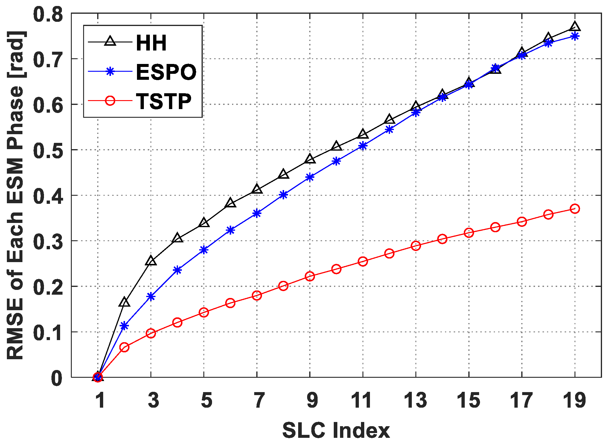
3.2. Simulated Experimental Result

To measure the phase improvement capability of different polarimetric optimization methods, this paper has estimated the RMSE of each ESM phase with Equation (23) according to the noise-free ESM interferometric phases with the S = 1000 independent simulations under the number of looks L = 60 and the temporal decorrelation threshold t h r e s = 100 . For the HH, the traditional ESPO, and the proposed TSTP algorithms, the overall RMSEs of the ESM phases are 0.428, 0.424, and 0.218, respectively. As shown in Figure 2, the optimization performance of the ESPO algorithm is close to the HH algorithm, and the phase denoising capability of the proposed TSTP method is better than the former two optimization methods significantly. Numerically, compared to the single polarimetric HH and the classical ESPO methods, the proposed TSTP method has obtained a higher optimization accuracy of 49.1% and 48.6%, respectively.

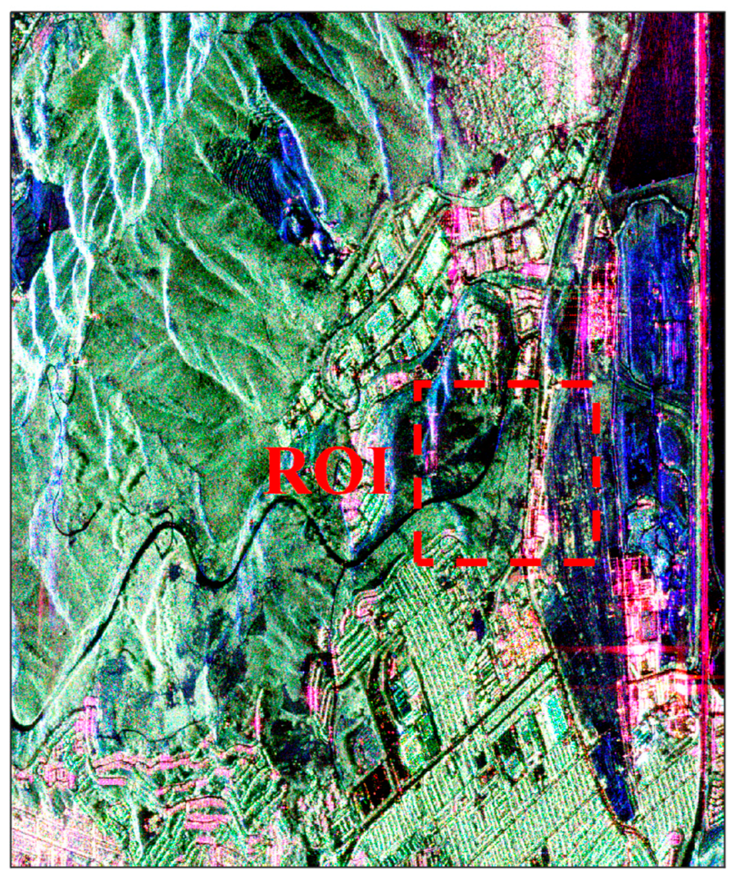
3.3. Real Experimental Data Description and Parameter Setting

In the real experiment, 12 scenes of ALOS PALSAR-2 L band full-polarimetric SAR image located in San Francisco, CA, USA, are acquired in the ascending passes, from 24 March 2015 to 25 June 2019. The pixel spacings in both the azimuth and range directions are 3.05 m and 2.86 m, respectively. Table 1 shows the image parameter list of time-series ALOS PALSAR-2 full polarimetric SAR data in detail. As shown in the Pauli basis RGB (PauliRGB) image of Figure 3, this paper selects a study area (1200 × 1000 pixels) containing complex buildings, mountains, bare lands, vegetation areas, etc.
In the following experiment, the 9th PolSAR acquisition on 18 April 2017, is taken as the master image and other acquisitions can be selected as slave ones to form all interferometric combinations, whose perpendicular and temporal baselines image is shown in Table 2. For the single-pass interferometric application, the TanDEM-X 90 m DEM data is used in the topographic phase simulation. Likewise, these three methods (i.e., the single polarimetric HH, the traditional ESPO, and the proposed TSTP methods) with the same parameter settings as the simulated experiment are applied to the Boxcar filtered TSPolInSAR data with a 7 × 7 local window, and the EMI method is performed for obtaining the ESM phases.

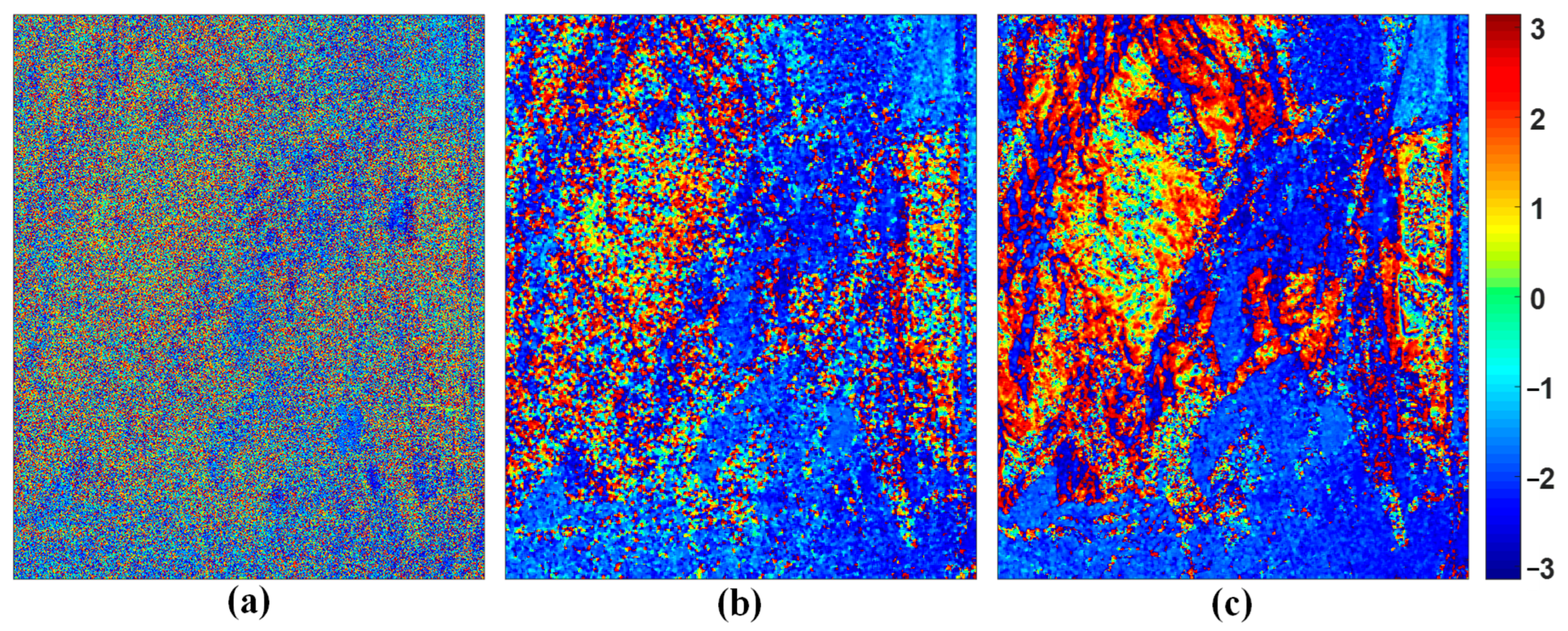
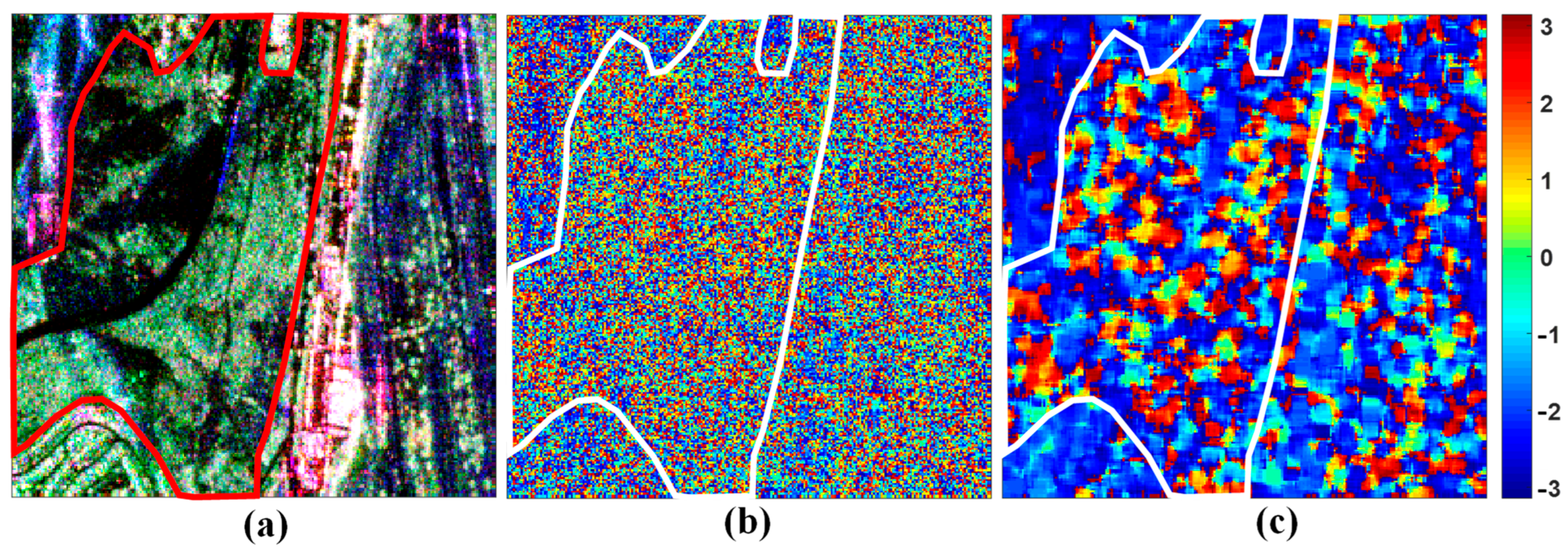
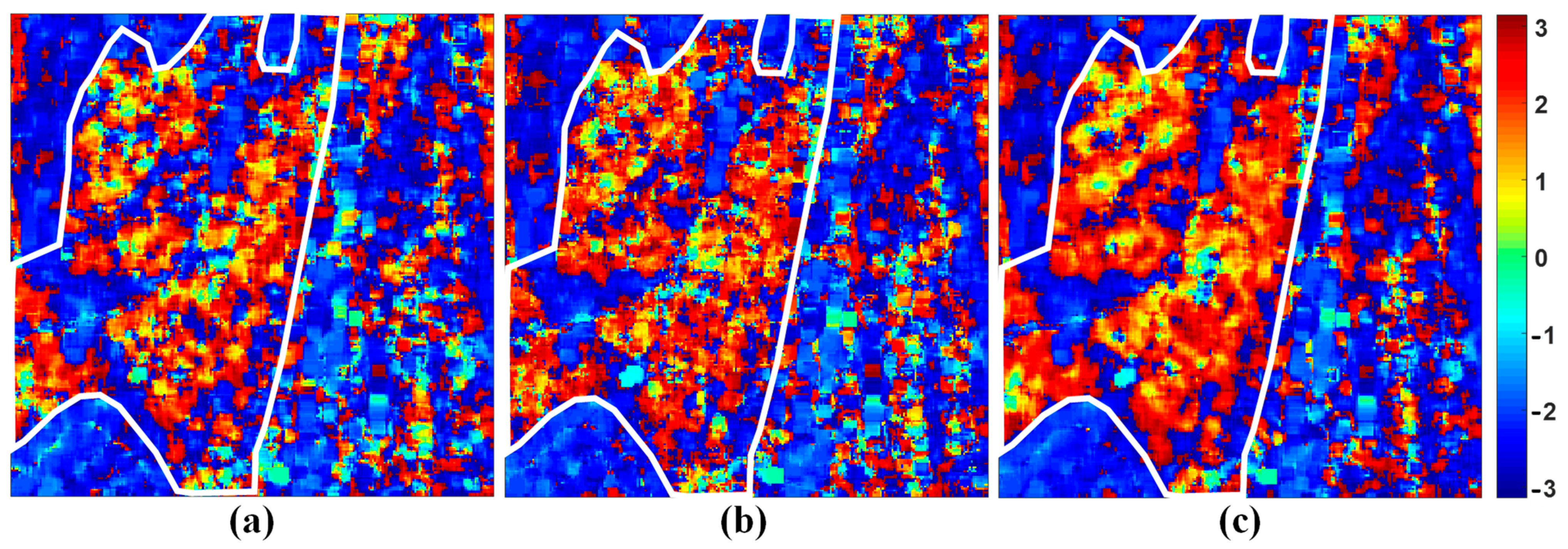
3.4. Real Experimental Result

Figure 4 displays the original and filtered interferograms in HH polarization and the optimized interferogram of the proposed TSTP method of the full scene between the 9th and 1st image observations. There is a significantly high phase noise level in the original interferogram in Figure 4a due to a temporal baseline of nearly two years. After performing the Boxcar filtering on the above interferogram between the 9th and 1st acquisitions, the filtered interferogram is essentially free of fringe phases in Figure 4b because of the limited denoising performance. As shown in Figure 4c, satisfactorily, the proposed TSTP algorithm can clearly recover the interferometric phase and effectively smooth the phase noise, even in the mountain area.

4. Discussion

The following compares the optimized results of three algorithms from the four aspects: (1) simulated experimental discussion under different multilooking size and decorrelation degrees, (2) real experimental discussion of the full scene, (3) real experimental discussion of the selected region of interest (ROI) marked by the red dotted box in Figure 3, and (4) computational efficiency comparison.

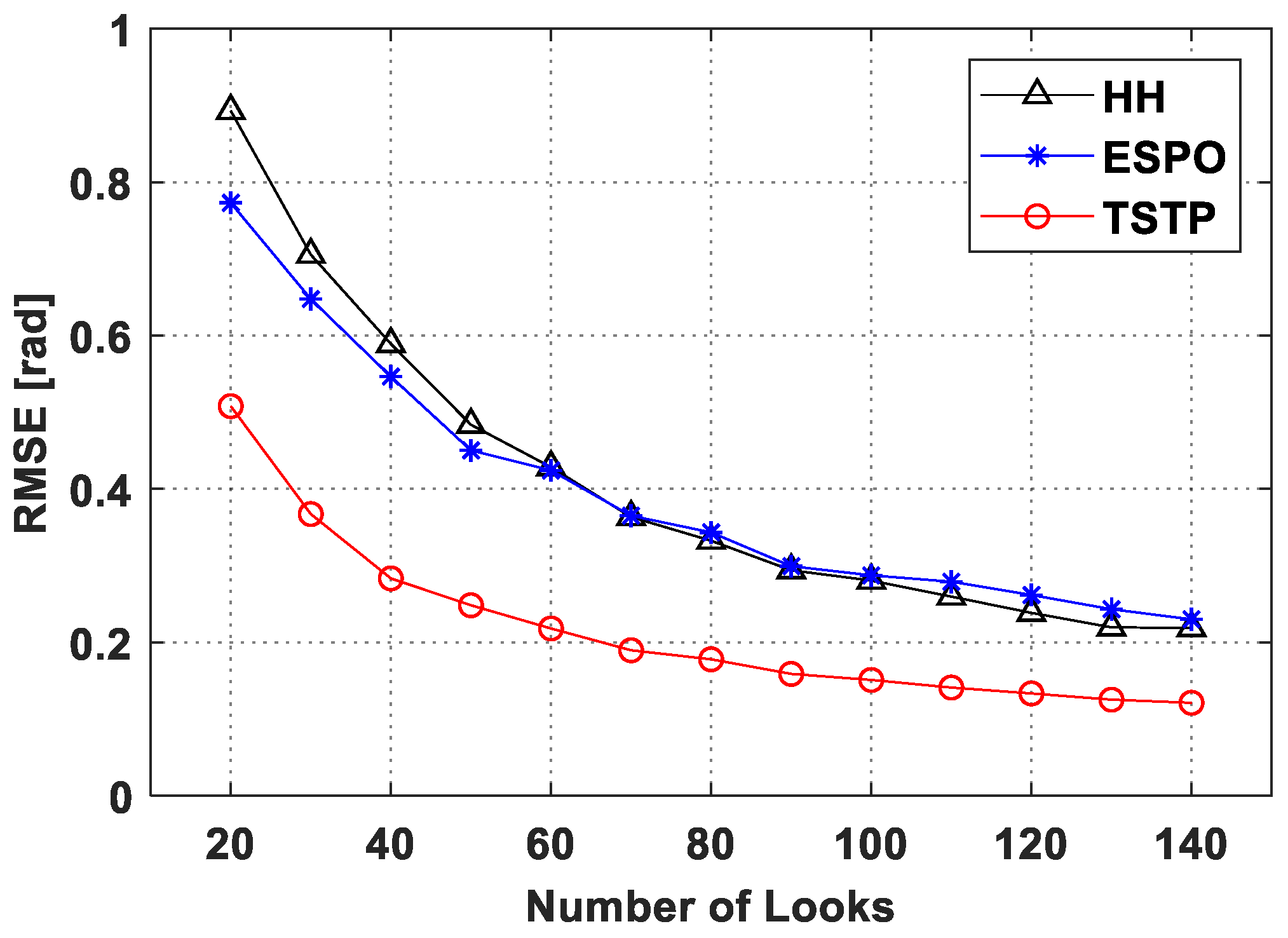
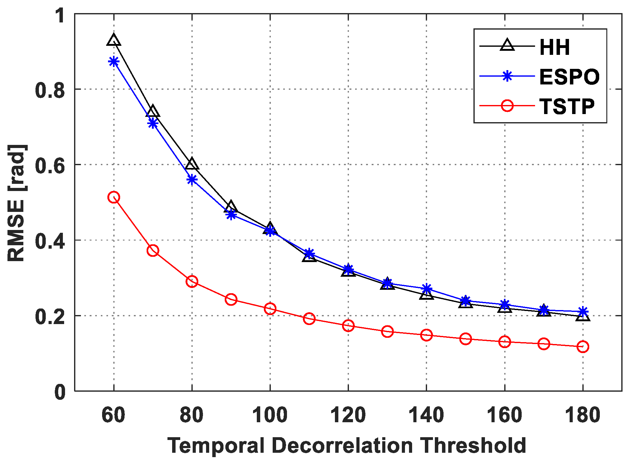
4.1. Simulated Experimental Discussion under Different Multilooking Size and Decorrelation Degrees

Based on the simulated experimental setting of Section 3.1, this section computes the overall RMSE of the ESM phases with Equation (24) to further measure the performance of three polarimetric optimizations quantitatively under different multilooking size and decorrelation degrees. To evaluate the optimization performance under different multilooking sizes, multiple experiments are simulated over various numbers of looks L = 20 : 10 : 140 and the temporal decorrelation threshold t h r e s = 100 . As shown in Figure 5, the ESPO method works better slightly than the HH method only at a low number of looks (i.e., L 60 ). Unfortunately, as the number of looks increases, the single-polarimetric HH method has slightly higher optimization performance, which means that the averaged coherence maximization-based ESPO method is unstable. On the whole, there is little difference in the ESM interferometric phase optimization between both HH and ESPO methods. However, the proposed TSTP method consistently achieves the lowest estimation error.
To further analyze the estimation accuracy under different decorrelation degrees, multiple experiments are simulated over the number of looks L = 60 and various temporal decorrelation thresholds t h r e s = 60 : 10 : 180 . It is seen from Figure 6 that both HH and ESPO methods have obtained similar ESM phase results, and the estimation error of the ESPO method is slightly lower than that of the HH method only in the case of severe decorrelation. However, the TSTP method always obtains the highest optimization level of the ESM phases. In summary, the proposed TSTP method is obviously superior to the previous two methods in all simulation cases.

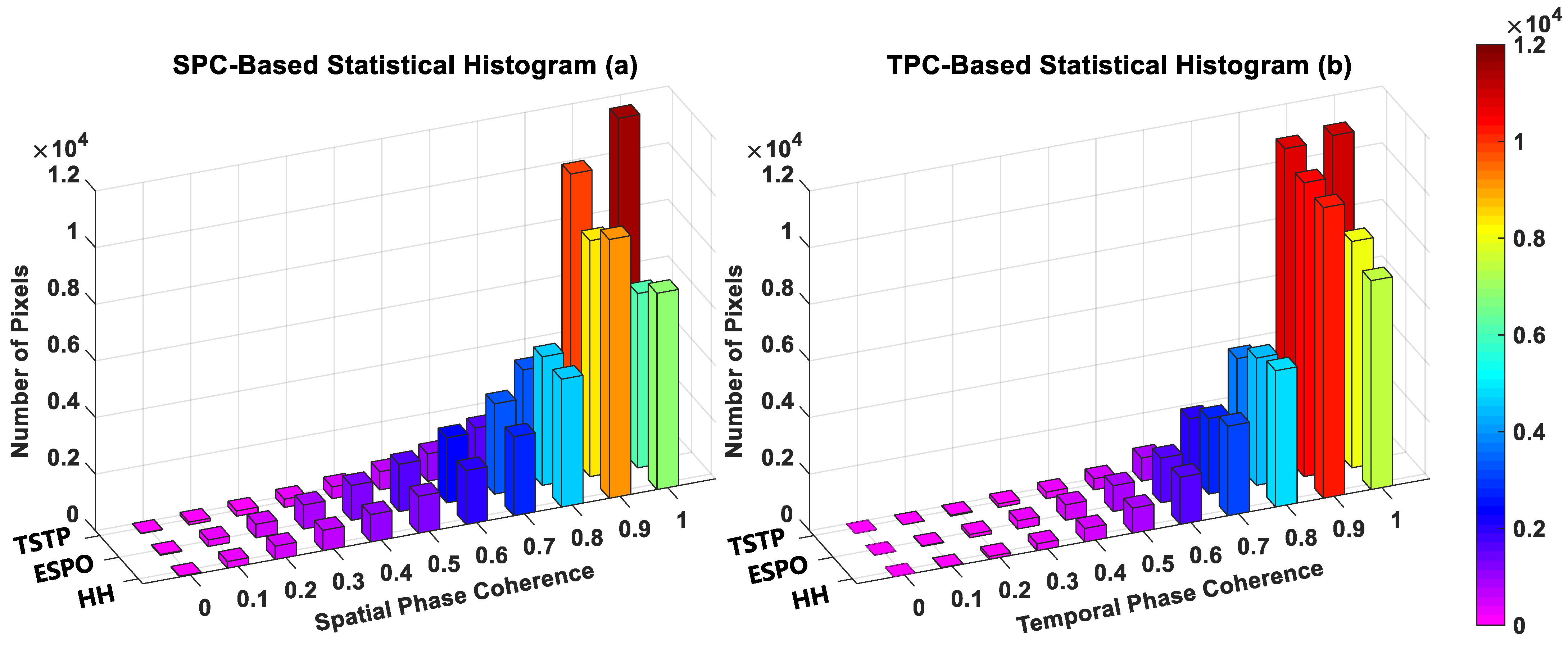
4.2. Real Experimental Discussion of The Full Scene

Based on the real experimental results of the full scene, this section analyzes the overall optimization performance of different methods from the following two aspects, including the coherence-based phase quality evaluation and the ENL difference between the single polarimetric TSIn and the TSTP coherency matrices.
Coherence-Based Phase Quality Evaluation: To quantitatively evaluate the optimization performance of different methods, we make statistics of the pseudo-coherence-based on the interferogram between the 9th and 1st acquisitions, also called the spatial phase coherence (SPC) in this paper, and temporal phase coherence (TPC) [15] to measure the degree of spatial and temporal smoothness of the optimized ESM phases, respectively. Based on the filtered or optimized interferogram between the 9th and 1st acquisitions, the SPC quality indicator can be computed with a local window K as follows [23]:
γ S P C = 1 K k K exp i ϕ k
where ϕ k is the interferometric phase for the kth pixel within the pixel set K. In addition, to evaluate the phase quality of a scatterer, the TPC quality indicator can be defined as follows [7,29]:
γ T P C = 1 M j = 1 M exp i ϕ j ϕ ¯ j ϕ ^ j , ε
where M is the selected interferometric pair set, ϕ ¯ j is the spatially filtered phase of the jth component ϕ j in the optimized ESM interferometric phases, and ϕ ^ j , ε is the residual phase corresponding to the external DEM errors.
In Figure 7, the number of pixels used in the coherence analysis is the same for each polarimetric optimization method, i.e., full image pixels (1200 × 1000 pixels). Therefore, under the premise of the same number of candidate pixels, if this method can be considered a better one, the level of coherence of all pixels will increase, and it will be seen from the estimated coherence histogram that the number of the highly coherent pixels increases and accordingly the number of the lowly coherent pixels decreases, which is an expected phenomenon. In Figure 7a, in terms of the overall degree of spatial smoothness of the optimized ESM phase, the numerical ranking of the estimated SPC levels is TSTP > HH > ESPO. In Figure 7b, in terms of the temporal smoothness effect of the optimized ESM phases, the numerical ranking of the estimated TPC levels is TSTP > ESPO > HH. Note that the ESPO method sometimes performs worse than the HH method due to the unstable statistical properties. Among three polarimetric optimization methods, the proposed TSTP method always keeps the highest coherence magnitude level in space and time.
ENL Difference between The Single Polarimetric TSIn and The TSTP Coherency Matrices: As mentioned in Section 2.2, the ENL can evaluate the speckle noise level of the coherency matrices accurately. The proposed TSTP method takes the polarimetric information as the statistical sample, and hence the stacking operator can increase the ENL level of the constructed TSTP coherency matrix. Therefore, according to the CRLB of the PL theory in Section 2.4 and Section 2.5, the optimization performance difference of the single-polarimetric TSIn and the TSTP coherency matrices can be determined by both ENLs of the original TSPolInSAR and the TSTP data, i.e., E N L T S I n and E N L T S T P , due to the degree of inter-channel correlation.
To quantitatively measure the difference of the speckle noise level between the TSIn coherency matrix in HH polarization and the proposed TSTP coherency matrix, this paper uses the TM estimator mentioned in Section 2.2 based on the original data to estimate E N L T S I n and E N L T S T P . As shown in Figure 8a,b, in terms of the overall effect, the E N L T S T P level is significantly greater than the E N L T S I n level. In addition, to directly evaluate the difference between the E N L T S T P and the E N L T S I n , we have made histogram statistics on the ratio of E N L T S T P to E N L T S I n , as shown in Figure 8c. It can be seen that the histogram peak is around 2.5, and the estimated ratio mean is 2.1, which is highlighted in red in the upper left corner of Figure 8c.

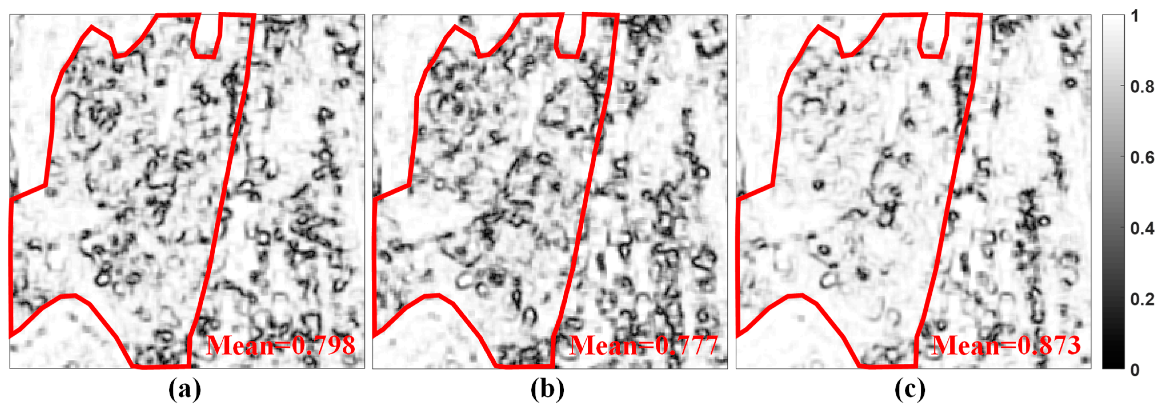
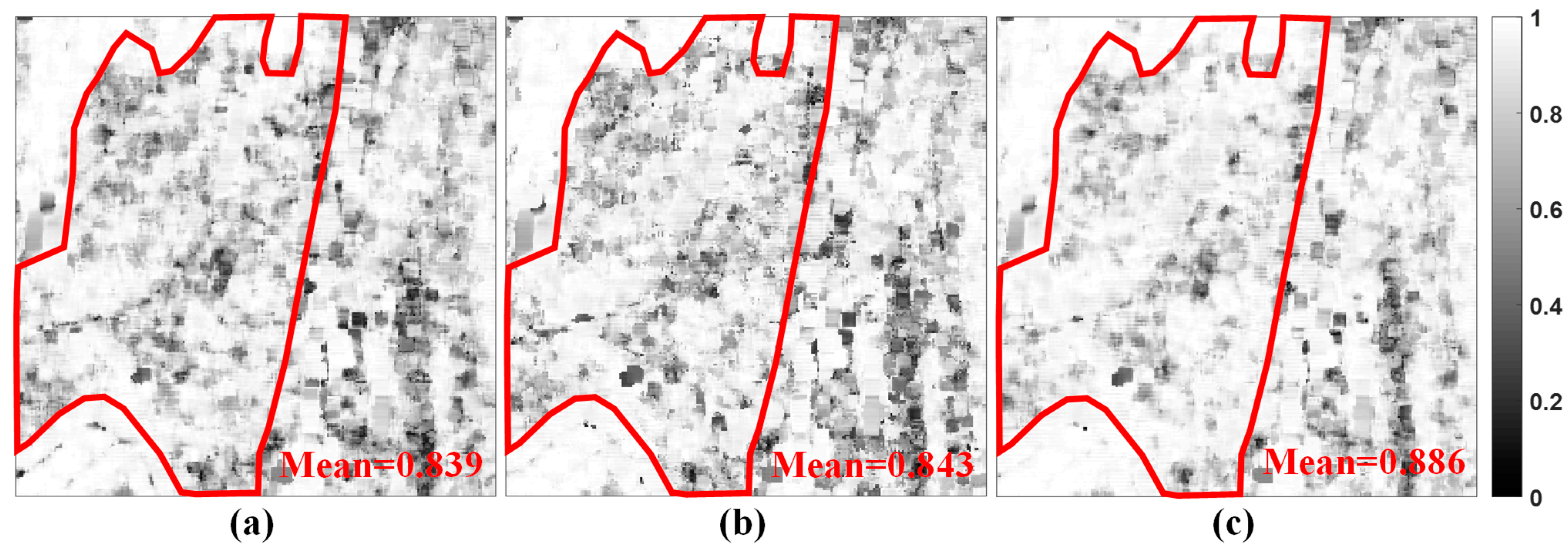
4.3. Real Experimental Discussion of The Selected ROI

For further investigation, the ROI with obvious structure features is selected by the red dotted box in the PauliRGB image of Figure 3, including the lowly coherent natural areas marked by the red irregular boxes in Figure 9a. Based on the experimental results of the selected ROI, this section analyzes the optimization performance of different methods from the following two aspects in detail, including the interferometric phase restoration and the coherence-based phase quality evaluation.
Interferometric Phase Restoration: It can be seen from Figure 9b that the serious decorrelation noise has also degraded the original interferogram in HH polarization seriously. Even the estimated interferometric fringe in Figure 9c with the Boxcar filtering cannot correspond to the textured structure in Figure 9a, which means that it is a challenging area for polarimetric optimization research.
Figure 10 shows the optimized interferograms of the selected ROI using different polarimetric optimizations (i.e., HH, ESPO, and proposed TSTP) between the 9th and 1st acquisitions. In the urban area, all methods obtain a smooth phase and good coherence estimates. However, in the natural scene, there are the speckle-like fluctuations and the spatial discontinuity phenomenon in both HH and ESPO optimized interferograms in Figure 10a,b, especially for the ESPO method. However, the TSTP method can recover the interferometric phase more clearly than the previous two methods, especially in the areas marked by the white irregular box in Figure 10c.
Coherence-Based Phase Quality Evaluation: Similar to the above Section 4.2, we also selected both SPC and TPC quality indicators to evaluate the phase improvement performance of different polarimetric optimization algorithms. Figure 11 and Figure 12 show the SPC images based on the estimated interferograms between the 9th and 1st acquisitions and the TPC image, respectively. There are 29,003 pixels in the selected natural area, and the estimated coherence means over the marked natural scene are also shown in Figure 11 and Figure 12.
In terms of phase quality, the polarimetric optimization capability of the ESPO method is unsatisfactory, especially in the marked natural scene in Figure 11 and Figure 12. The SPC level is lower than that of the HH method even though the TPC level is slightly higher than that of the HH method. Hence, in terms of the SPC level based on the interferogram between the 9th and 1st acquisitions, the numerical ranking of the mean values is TSTP > HH > ESPO. In terms of the TPC level based on the optimized ESM phases, the numerical ranking of the mean values is TSTP > ESPO > HH. Additionally, we make the coherence-based histogram statistics over the selected natural scene in Figure 13, including the SPC and TPC histograms. Among all methods, the proposed TSTP method achieves the highest coherence level.

4.4. Computational Efficiency Comparison between Two Polarimetric Optimization Methods

With the help of the commercial GAMMA software, the time-series polarimetric SLC stack is generated from the raw data, and the corresponding topographic and orbital phase components are also removed with the TanDEM-X 90m DEM data and the orbital information, respectively. Based on the SLC stack generated above, the optimization processes of both ESPO and TSTP methods are achieved by the MATLAB 2018a programming software under the hardware configuration of a single-core Intel Core i7-6800K 3.4 GHz CPU and 80 GB RAM. Table 3 displays the significant efficiency of the proposed TSTP method over the traditional ESPO method. Because the proposed method does not require a pixel-by-pixel search as the ESPO method does, it just needs to stack all the whole imagery TSIn coherency matrices over full polarizations.

5. Conclusions

With the increase of the time-series polarimetric SAR data, many scholars have focused on the utilization of polarimetric information to improve the interferometric phase quality of a ground target, called the polarimetric optimization methods. Traditional polarimetric optimization methods usually take the quality indicator as the optimization criterion to search for an optimal polarimetric channel in the given polarimetric domain. However, the optimization performance of the traditional quality indicator-based polarimetric optimization methods is limited by the unstable statistical properties and the huge computation cost. According to the CRLB of the PL, the optimization performance of DS’s time-series interferometric phases depends on the number of looks and the time-series coherence magnitude matrix. In contrast to the traditional coherence magnitude-based ESPO method, this paper proposes considering polarimetric information as statistical samples and stacking the TSIn coherency matrices over full polarimetric channels to construct the TSTP coherency matrix for optimizing the ESM interferometric phases. The novel TSTP coherency matrix has abundant theoretical values, which can represent the TSIn coherency matrix of the center of mass of the CR and suppress the SNR decorrelation. Simulated and real experimental results and discussions verified the superior performance and computational efficiency of time-series interferometric phase optimization, especially in the natural scene with severe decorrelation.

Author Contributions

Methodology, P.S.; software, P.S.; validation, P.S.; visualization, P.S.; formal analysis, P.S. and C.W.; supervision, C.W. and J.H.; writing—original draft, P.S.; writing—review and editing, C.W. and J.H. All authors have read and agreed to the published version of the manuscript.

Funding

This research was funded by the National Natural Science Foundation of China (No. 42030112, 41671356), Natural Science Foundation of Hunan province, China (No. 2022JJ30705), the Fundamental Research Funds for the Central Universities of Central South University (No. 2021zzts0255), and the Postgraduate Scientific Research Innovation Project of Hunan Province (No. CX20210273).

Data Availability Statement

The ALOS PALSARS-2 full polarimetric SAR data presented in this study was obtained from the Japan Aerospace Exploration Agency (JAXA)’s Earth Observation Campaigns Data Project and are available with the permission of the JAXA.

Acknowledgments

The authors would like to thank the Japan Aerospace Exploration Agency (JAXA) for providing ALOS PALSARS-2 full polarimetric SAR data under science proposals (ER3A2N032 and ER3A2N141). They would like to thank the German Aerospace Cencter (DLR) for providing the TanDEM-X 90m DEM data.

Conflicts of Interest

The authors declare no conflict of interest.

References

  1. Zebker, H.A.; Villasenor, J. Decorrelation in interferometric radar echoes. IEEE Trans. Geosci. Remote Sens. 1992, 30, 950–959. [Google Scholar] [CrossRef]
  2. Hanssen, R.F. Radar Interferometry: Data Interpretation and Error Analysis; Springer Science & Business Media: Berlin, Germany, 2001; ISBN 0792369459. [Google Scholar]
  3. Ferretti, A.; Prati, C.; Rocca, F. Nonlinear subsidence rate estimation using permanent scatterers in differential SAR interferometry. IEEE Trans. Geosci. Remote Sens. 2000, 38, 2202–2212. [Google Scholar] [CrossRef]
  4. Ferretti, A.; Prati, C.; Rocca, F. Permanent scatterers in SAR interferometry. IEEE Trans. Geosci. Remote Sens. 2001, 39, 8–20. [Google Scholar] [CrossRef]
  5. Werner, C.; Wegmuller, U.; Strozzi, T.; Wiesmann, A. Interferometric point target analysis for deformation mapping. In Proceedings of the IGARSS 2003. 2003 IEEE International Geoscience and Remote Sensing Symposium. Proceedings, Toulouse, France, 21–25 July 2003; pp. 4362–4364. [Google Scholar]
  6. Costantini, M.; Falco, S.; Malvarosa, F.; Minati, F. A new method for identification and analysis of persistent scatterers in series of SAR images. In Proceedings of the IGARSS 2008—2008 IEEE International Geoscience and Remote Sensing Symposium, Boston, MA, USA, 7–11 July 2008; pp. II-449–II–452. [Google Scholar]
  7. Hooper, A.; Zebker, H.; Segall, P.; Kampes, B. A new method for measuring deformation on volcanoes and other natural terrains using InSAR persistent scatterers. Geophys. Res. Lett. 2004, 31, L23611. [Google Scholar] [CrossRef]
  8. Hooper, A.; Segall, P.; Zebker, H. Persistent scatterer interferometric synthetic aperture radar for crustal deformation analysis, with application to Volcan Alcedo, Galapagos. J. Geophys. Res. Earth 2007, 112, B07407. [Google Scholar] [CrossRef]
  9. Berardino, P.; Fornaro, G.; Lanari, R.; Sansosti, E. A new algorithm for surface deformation monitoring based on small baseline differential SAR interferograms. IEEE Trans. Geosci. Remote Sens. 2002, 40, 2375–2383. [Google Scholar] [CrossRef]
  10. Lanari, R.; Mora, O.; Manunta, M.; Mallorqui, J.J.; Berardino, P.; Sansosti, E. A small-baseline approach for investigating deformations on full-resolution differential SAR interferograms. IEEE Trans. Geosci. Remote Sens. 2004, 42, 1377–1386. [Google Scholar] [CrossRef]
  11. Xiao, R.; Jiang, M.; Li, Z.; He, X. New insights into the 2020 Sardoba dam failure in Uzbekistan from Earth observation. Int. J. Appl. Earth Obs. Geoinf. 2022, 107, 102705. [Google Scholar] [CrossRef]
  12. Blanco-Sanchez, P.; Mallorqui, J.J.; Duque, S.; Monells, D. The Coherent Pixels Technique (CPT): An advanced DInSAR technique for nonlinear deformation monitoring. Pure Appl. Geophys. 2008, 165, 1167–1193. [Google Scholar] [CrossRef]
  13. Ferretti, A.; Fumagalli, A.; Novali, F.; Prati, C.; Rocca, F.; Rucci, A. A New Algorithm for Processing Interferometric Data-Stacks: SqueeSAR. IEEE Trans. Geosci. Remote Sens. 2011, 49, 3460–3470. [Google Scholar] [CrossRef]
  14. Zhang, L.; Ding, X.; Lu, Z. Modeling PSInSAR time series without phase unwrapping. IEEE Trans. Geosci. Remote Sens. 2011, 49, 547–556. [Google Scholar] [CrossRef]
  15. Zhang, L.; Lu, Z.; Ding, X.; Jung, H.; Feng, G.; Lee, C.-W. Mapping ground surface deformation using temporarily coherent point SAR interferometry: Application to Los Angeles Basin. Remote Sens. Environ. 2012, 117, 429–439. [Google Scholar] [CrossRef]
  16. Guarnieri, A.M.; Tebaldini, S. On the exploitation of target statistics for SAR interferometry applications. IEEE Trans. Geosci. Remote Sens. 2008, 46, 3436–3443. [Google Scholar] [CrossRef]
  17. Jiang, M.; Ding, X.; Hanssen, R.F.; Malhotra, R.; Chang, L. Fast statistically homogeneous pixel selection for covariance matrix estimation for multitemporal InSAR. IEEE Trans. Geosci. Remote Sens. 2015, 53, 1213–1224. [Google Scholar] [CrossRef]
  18. Dong, J.; Liao, M.; Zhang, L.; Gong, J. A unified approach of multitemporal sar data filtering through adaptive estimation of complex covariance matrix. IEEE Trans. Geosci. Remote Sens. 2018, 56, 5320–5333. [Google Scholar] [CrossRef]
  19. Fornaro, G.; Verde, S.; Reale, D.; Pauciullo, A. CAESAR: An approach based on covariance matrix decomposition to improve multibaseline-multitemporal interferometric SAR processing. IEEE Trans. Geosci. Remote Sens. 2015, 53, 2050–2065. [Google Scholar] [CrossRef]
  20. Ansari, H.; De Zan, F.; Bamler, R. Efficient Phase Estimation for Interferogram Stacks. IEEE Trans. Geosci. Remote Sens. 2018, 56, 4109–4125. [Google Scholar] [CrossRef]
  21. Jiang, M.; Guarnieri, A.M. Distributed Scatterer Interferometry with the Refinement of Spatiotemporal Coherence. IEEE Trans. Geosci. Remote Sens. 2020, 58, 3977–3987. [Google Scholar] [CrossRef]
  22. Ansari, H.; Zan, F.D.; Bamler, R. Sequential Estimator: Toward Efficient InSAR Time Series Analysis. IEEE Trans. Geosci. Remote Sens. 2017, 55, 5637–5652. [Google Scholar] [CrossRef]
  23. Neumann, M.; Ferro-Famil, L.; Reigber, A. Multibaseline polarimetric SAR interferometry coherence optimization. IEEE Geosci. Remote Sens. Lett. 2008, 5, 93–97. [Google Scholar] [CrossRef] [Green Version]
  24. Navarro-Sanchez, V.D.; Lopez-Sanchez, J.M.; Vicente-Guijalba, F. A contribution of polarimetry to satellite differential SAR interferometry: Increasing the number of pixel candidates. IEEE Geosci. Remote Sens. Lett. 2010, 7, 276–280. [Google Scholar] [CrossRef]
  25. Navarro-Sanchez, V.D.; Lopez-Sanchez, J.M. Improvement of persistent-scatterer interferometry performance by means of a polarimetric optimization. IEEE Geosci. Remote Sens. Lett. 2012, 9, 609–613. [Google Scholar] [CrossRef]
  26. Iglesias, R.; Monells, D.; Fabregas, X.; Mallorqui, J.J.; López-Martínez, C. Phase Quality Optimization in Polarimetric Differential SAR Interferometry. IEEE Trans. Geosci. Remote Sens. 2014, 52, 2875–2888. [Google Scholar] [CrossRef]
  27. Zhao, F.; Mallorqui, J.J. Coherency matrix decomposition-based polarimetric persistent scatterer interferometry. IEEE Trans. Geosci. Remote Sens. 2019, 57, 7819–7831. [Google Scholar] [CrossRef]
  28. Wu, B.; Tong, L.; Chen, Y.; He, L. New Methods in Multibaseline Polarimetric SAR Interferometry Coherence Optimization. IEEE Geosci. Remote Sens. Lett. 2015, 12, 2016–2020. [Google Scholar] [CrossRef]
  29. Sadeghi, Z.; Zoej, M.J.V.; Hooper, A.; Lopez-Sanchez, J.M. A new polarimetric persistent scatterer interferometry method using temporal coherence optimization. IEEE Trans. Geosci. Remote Sens. 2018, 56, 6547–6555. [Google Scholar] [CrossRef]
  30. Shen, P.; Wang, C.; Hu, J.; Fu, H.; Zhu, J. Interferometric Phase Optimization Based on PolInSAR Total Power Coherency Matrix Construction and Joint Polarization-Space Nonlocal Estimation. IEEE Trans. Geosci. Remote Sens. 2022, 60, 5201014. [Google Scholar] [CrossRef]
  31. Shen, P.; Wang, C.; Lu, L.; Luo, X.; Hu, J.; Fu, H.; Zhu, J. A Novel Polarimetric PSI Method Using Trace Moment-Based Statistical Properties and Total Power Interferogram Construction. IEEE Trans. Geosci. Remote Sens. 2022, 60, 4402815. [Google Scholar] [CrossRef]
  32. Guarnieri, A.M.; Tebaldini, S. Hybrid Cramér-Rao bounds for crustal displacement field estimators in SAR interferometry. IEEE Signal Process. Lett. 2007, 14, 1012–1015. [Google Scholar] [CrossRef]
  33. Lee, J.S.; Pottier, E. Polarimetric Radar Imaging: From Basics to Applications; CRC Press: Boca Raton, FL, USA, 2009. [Google Scholar]
  34. Lee, J.S.; Hoppel, K.W.; Mango, S.A.; Miller, A.R. Intensity and phase statistics of multilook polarimetric and interferometric SAR imagery. IEEE Trans. Geosci. Remote Sens. 1994, 32, 1017–1028. [Google Scholar] [CrossRef]
  35. Oliver, C.; Quegan, S. Understanding Synthetic Aperture Radar Images, 2nd ed.; SciTech Publishing: Raleigh, NC, USA, 2004. [Google Scholar]
  36. Anfinsen, S.N.; Doulgeris, A.P.; Eltoft, T. Estimation of the equivalent number of looks in polarimetric synthetic aperture radar imagery. IEEE Trans. Geosci. Remote Sens. 2009, 47, 3795–3809. [Google Scholar] [CrossRef]
  37. Shen, P.; Wang, C.; Fu, H.; Zhu, J.; Hu, J. Estimation of Equivalent Number of Looks in Time-Series Pol(In)SAR Data. Remote Sens. 2020, 12, 2715. [Google Scholar] [CrossRef]
  38. Gao, H.; Wang, C.; Xiang, D.; Ye, J.; Wang, G. TSPol-ASLIC: Adaptive Superpixel Generation with Local Iterative Clustering for Time-Series Quad- and Dual-Polarization SAR Data. IEEE Trans. Geosci. Remote Sens. 2022, 60, 5217015. [Google Scholar] [CrossRef]
  39. Maiwald, D.; Kraus, D. Calculation of moments of complex Wishart and complex inverse Wishart distributed matrices. IEE Proc. Radar Sonar Navig. 2000, 147, 162–168. [Google Scholar] [CrossRef]
  40. Marino, A. Trace Coherence: A New Operator for Polarimetric and Interferometric SAR images. IEEE Trans. Geosci. Remote Sens. 2017, 55, 2326–2339. [Google Scholar] [CrossRef]
  41. Tao, X.; Jian, Y.; Weijie, Z. Interferometric Phase Improvement Based on Polarimetric Data Fusion. Sensors 2008, 8, 7172–7190. [Google Scholar] [CrossRef]
  42. Kwok, R.; Lee, J.S.; Grunes, M.R. Classification of Multi-Look Polarimetric SAR Imagery Based on Complex Wishart Distribution. Int. J. Remote Sens. 1994, 15, 2299–2312. [Google Scholar] [CrossRef]
Figure 1. The flowchart of the proposed TSTP method.
Remotesensing 14 04168 g001
Figure 2. RMSE comparison of each ESM phase using the HH, ESPO, and proposed TSTP algorithms under the number of looks L = 60 and the temporal decorrelation threshold t h r e s = 100 .
Remotesensing 14 04168 g002
Figure 3. Temporally averaged PauliRGB image of ALOS PALSAR-2 TSPolInSAR data. The region of interest (ROI) (250 × 250 pixels) marked by the dotted box is selected for the following further investigation in Section 4.3.
Remotesensing 14 04168 g003
Figure 4. Estimated interferograms of the full scene between the 9th and 1st image observations. (a) Original interferogram in HH polarization. (b) Estimated interferogram in HH polarization with the Boxcar filtering. (c) Optimized interferogram of the proposed TSTP method.
Remotesensing 14 04168 g004
Figure 5. Estimated overall RMSEs of different methods under multiple numbers of looks L = 20 : 10 : 140 and the temporal decorrelation threshold t h r e s = 100 .
Remotesensing 14 04168 g005
Figure 6. Estimated overall RMSEs of different methods under the number of looks L = 60 and multiple temporal decorrelation thresholds t h r e s = 60 : 10 : 180 .
Remotesensing 14 04168 g006
Figure 7. Estimated coherence histograms of the full scene under different methods (i.e., HH, ESPO, and proposed TSTP). (a) SPC. (b) TPC. Under the premise of the same number of candidate pixels, if this method is considered a better one, it can be seen from the histogram that the number of the highly coherent pixels increases, and accordingly the number of the lowly coherent pixels decreases.
Remotesensing 14 04168 g007
Figure 8. Estimated ENL images of full scene based on (a) the original TSIn coherency matrices in the HH polarization and (b) the original TSTP coherency matrices, and the corresponding ratio histogram (c) of E N L T S T P to E N L T S I n .
Remotesensing 14 04168 g008
Figure 9. The original PauliRGB image (a), the original (b), and the Boxcar filtered (c) interferograms between the 9th and 1st acquisitions of ROI (250 × 250 pixels). The lowly coherent natural area is marked by the irregular box in Figure 9a–c.
Remotesensing 14 04168 g009
Figure 10. Optimized interferograms between the 9th and 1st acquisitions of ROI (250 × 250 pixels) using (a) HH, (b) ESPO, and (c) proposed TSTP methods. The lowly coherent natural area is marked by the white irregular box in Figure 10a–c.
Remotesensing 14 04168 g010
Figure 11. Estimated SPC images of ROI (250 × 250 pixels) using (a) HH, (b) ESPO, and (c) proposed TSTP methods. The estimated SPC means over the natural scene are shown in Figure 11. The lowly coherent natural area is marked by the red irregular boxes in Figure 11a–c.
Remotesensing 14 04168 g011
Figure 12. Estimated TPC images of ROI (250 × 250 pixels) using (a) HH, (b) ESPO, and (c) proposed TSTP methods. The estimated TPC means over the natural scene are shown in Figure 12. The lowly coherent natural area is marked by the red irregular box in Figure 12a–c.
Remotesensing 14 04168 g012
Figure 13. Estimated coherence histograms of the marked natural area by the red irregular boxes in Figure 9a under different methods (i.e., HH, ESPO, and proposed TSTP). (a) SPC. (b) TPC. Under the premise of the same number of candidate pixels, if this method is considered a better one, it can be seen from the histogram that the number of the highly coherent pixels increases, and accordingly the number of the lowly coherent pixels decreases.
Remotesensing 14 04168 g013
Table 1. Image Parameter List of Time-Series ALOS PALSAR-2 Full Polarimetric SAR data.
SensorPolarizationNumber
of Images
FrequencyRange SpacingAzimuth
Spacing
Incident Angle
ALOS
PALSAR-2
Full121.24 GHz2.86 m3.05 m33.24°
Table 2. Perpendicular and Temporal Baseline List of ALOS PALSAR-2 TSPolInSAR data.
Acquisition TimePerpendicular Baseline (m)Temporal Baseline (Day)
2015032429.5−756
2016020930.2−434
20160223−260.4−420
20160809−33.0−252
2016100426.6−196
2016110128.1−168
20170124−51.8−84
20170404225.7−14
2017041800
20170822−64.7126
201808216.0490
20190625−112.4798
The image with the acquisition time in bold is selected as the master one.
Table 3. Cost Time Comparison Between Different Polarimetric Optimization Methods.
MethodALOS PALSAR-2 (1200 × 1000 pixels)
ESPO1,408,181.04 s
TSTP2.28 s
Publisher’s Note: MDPI stays neutral with regard to jurisdictional claims in published maps and institutional affiliations.

