
A Hybrid Model Based on Superpixel Entropy Discrimination for PolSAR Image Classification


Abstract
:1. Introduction
- (1)
- A superpixel entropy discrimination method was proposed, and the definition of superpixel entropy based on information entropy was proposed to describe the evidence conflict in a single superpixel, which was used to evaluate the quality of superpixel classification.
- (2)
- A two-level cascade classifier based on LGBM+SLIC and CV-CNN was proposed. The superpixels with high entropy were reclassified by CV-CNN to reduce the accuracy loss caused by evidence conflict in a single superpixel.
- (3)
- The training and testing time consumption of LGBM+SLIC were short. The integrated model could achieve the same accuracy by using CV-CNN for the whole image, which greatly shortened the testing time while maintaining high-accuracy performance.
2. Proposed Method
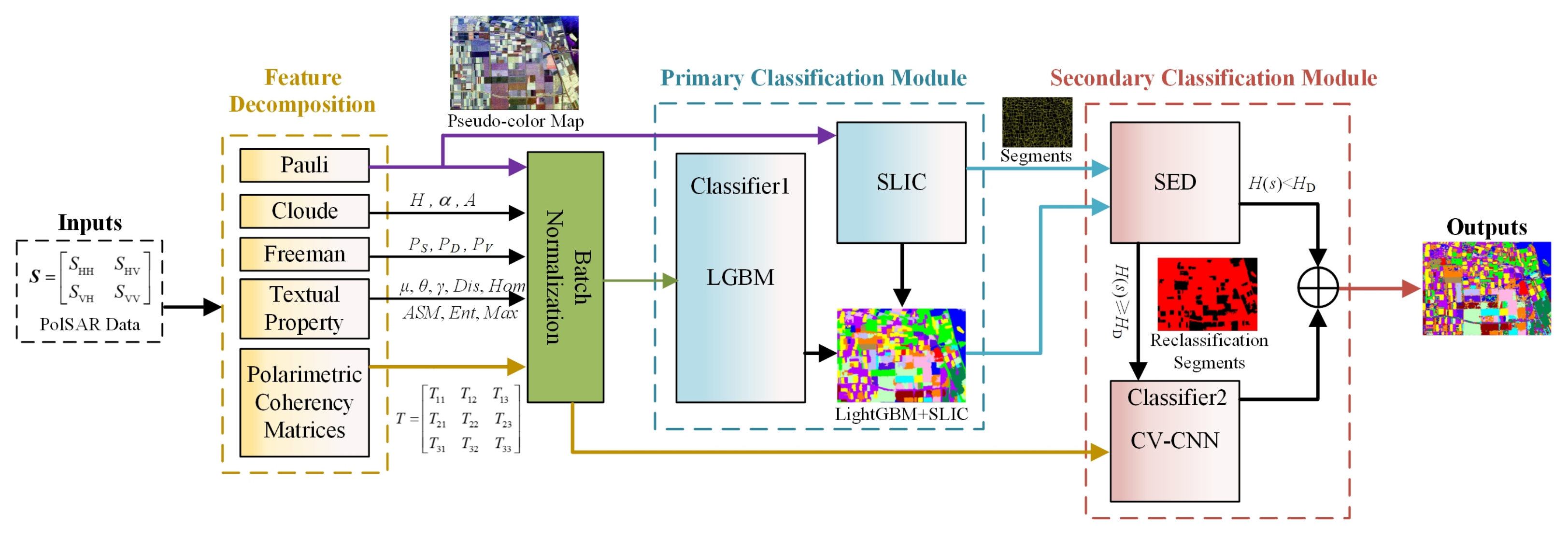
2.1. Main Framework
2.2. Feature Decomposition
2.3. Primary Classification Module
2.3.1. Light Gradient Boosting Machine (LGBM)
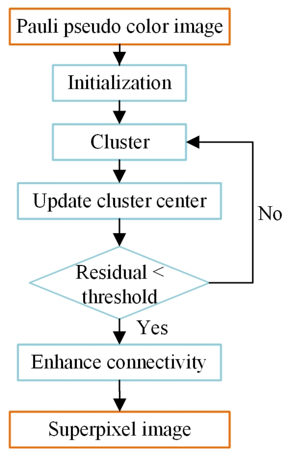
2.3.2. Simple Linear Iterative Clustering(SLIC)
2.4. Secondary Classification Module
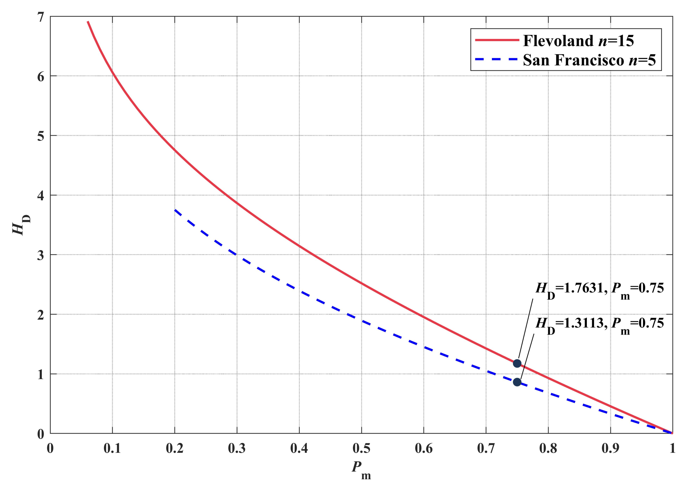
2.4.1. Superpixel Entropy Discrimination(SED)
- (1)
- If , it means that a classification dominates in a single superpixel. The superpixel has high classification quality. The uncertainty in this superpixel is mainly caused by speckle noise or small-scale classification errors of the primary classifier. It is feasible to use the maximum classification instead of local region classification.
- (2)
- If , it means that multiple classifications may account for similar proportions in a single superpixel. The kind of superpixel has low classification quality. The uncertainty in this superpixel is mainly caused by the error of superpixel edge segmentation or the large-scale classification error of the primary classifier. It is not feasible to use the maximum classification to replace the local area. We used CV-CNN to reclassify it.
2.4.2. Complex-Valued Convolutional Neural Network (CV-CNN)
3. Experiments and Results
3.1. Experimental Setup
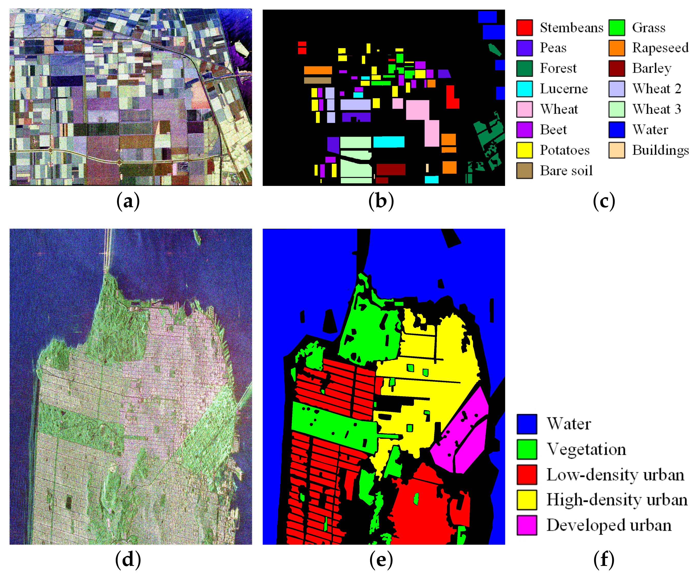
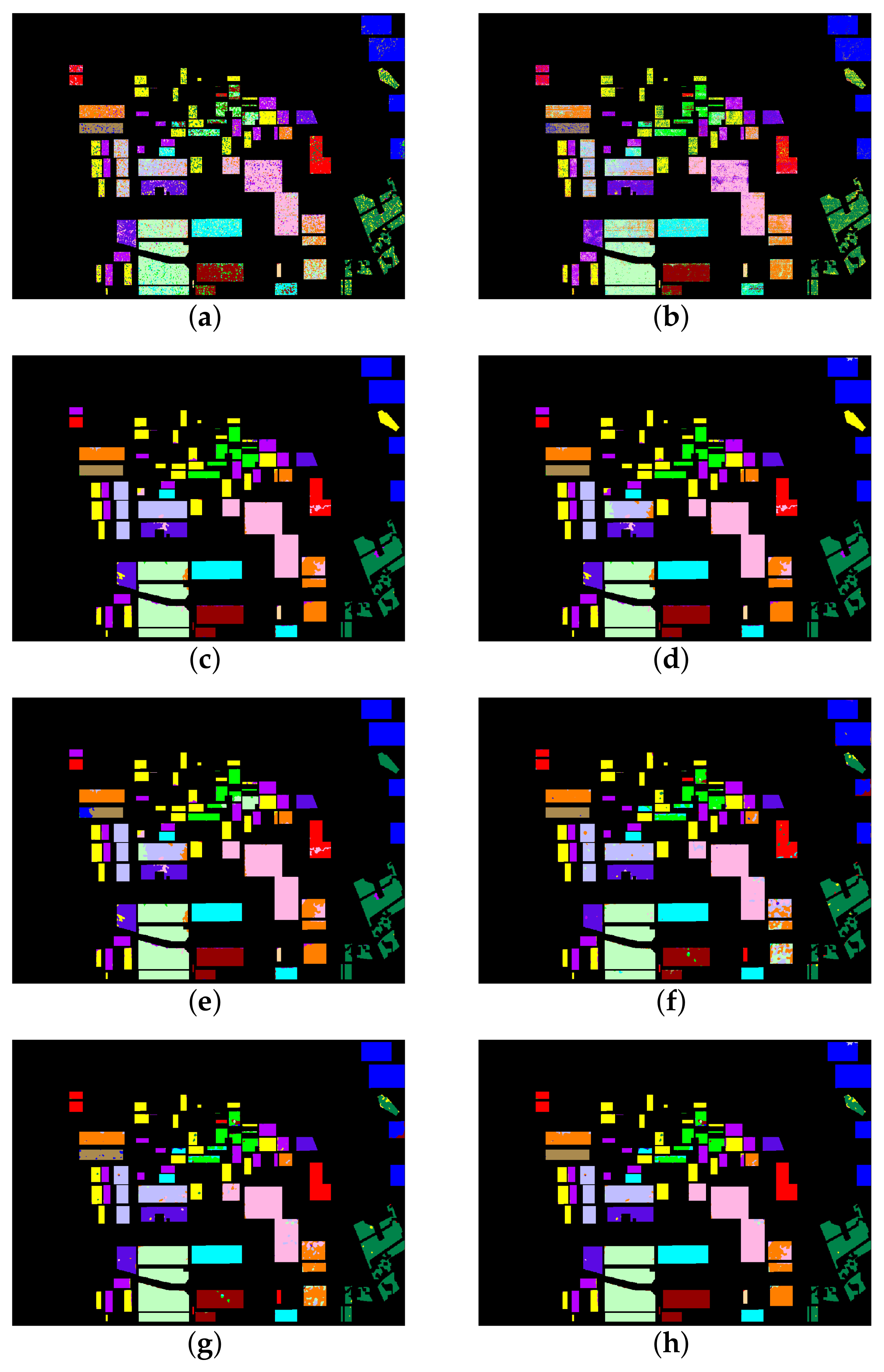
3.2. Classification Results of Flevoland Dataset
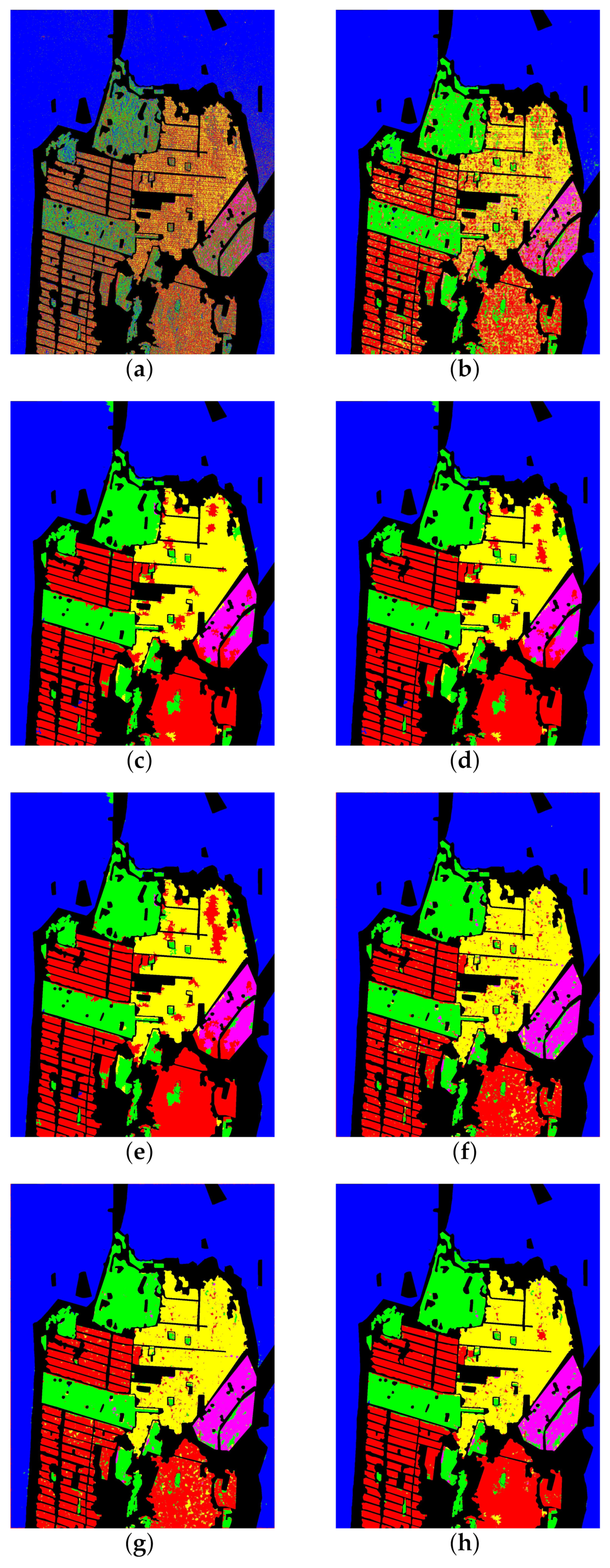
3.3. Classification Results of San Francisco Dataset
4. Disussion
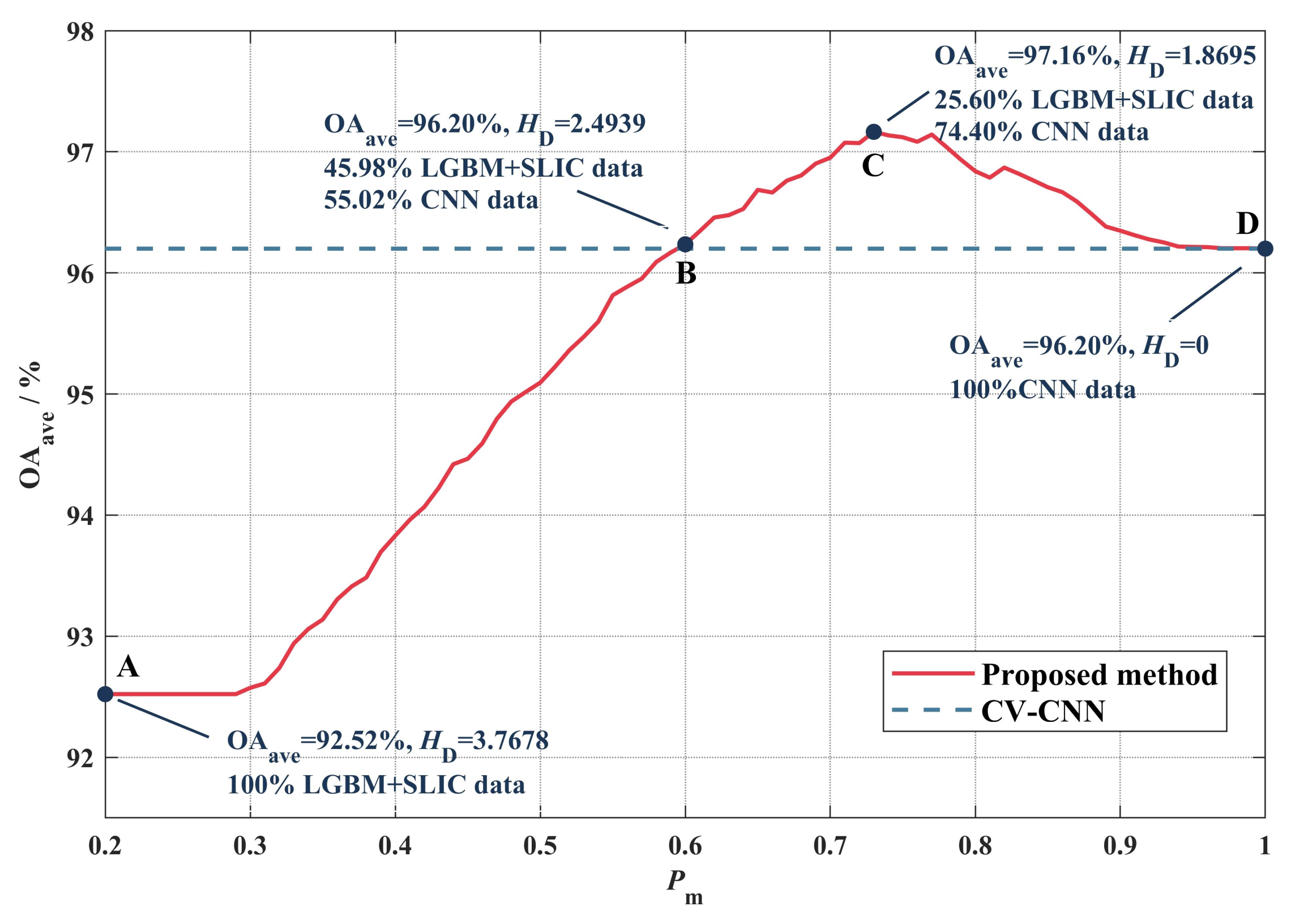
4.1. Classification Effect of SED
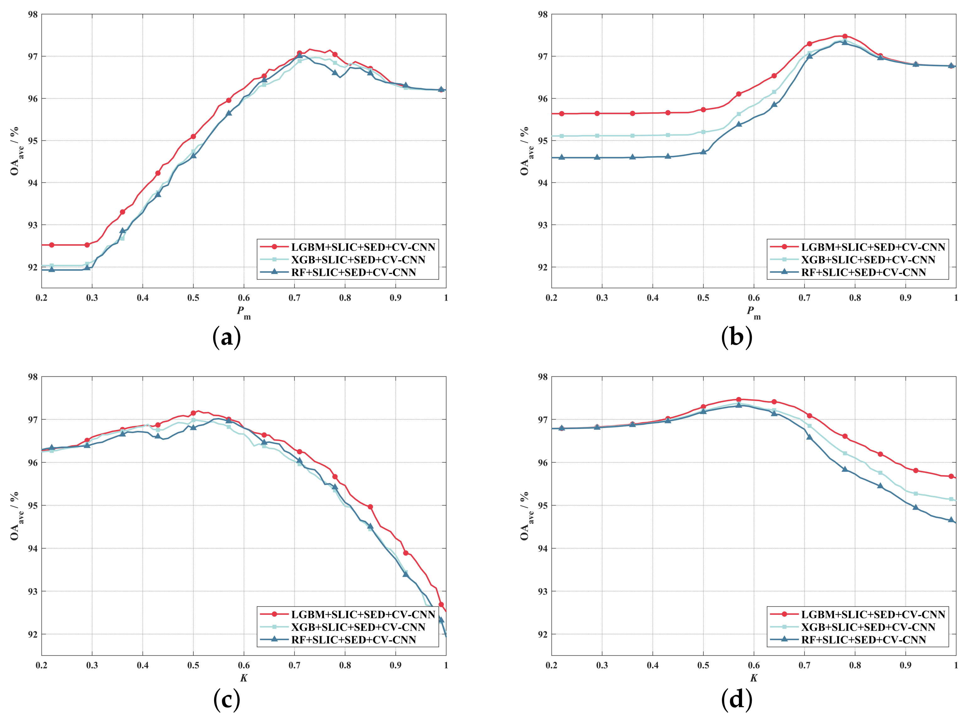
4.2. Configuration of SED
5. Conclusions
Author Contributions
Funding
Institutional Review Board Statement
Informed Consent Statement
Data Availability Statement
Acknowledgments
Conflicts of Interest
References
- Pierce, L.E.; Ulaby, F.T.; Sarabandi, K.; Dobson, M.C. Knowledge-based classification of polarimetric SAR images. IEEE Trans. Geosci. Remote Sens. 1994, 32, 1081–1086. [Google Scholar] [CrossRef]
- Cloude, S.R.; Pottier, E. An entropy based classification scheme for land applications of polarimetric SAR. IEEE Trans. Geosci. Remote Sens. 1997, 35, 68–78. [Google Scholar] [CrossRef]
- Zhai, W.; Shen, H.; Huang, C.; Pei, W. Fusion of polarimetric and texture information for urban building extraction from fully polarimetric SAR imagery. Remote Sens. Lett. 2016, 7, 31–40. [Google Scholar] [CrossRef]
- Quan, S.; Xiong, B.; Xiang, D.; Zhao, L.; Zhang, S.; Kuang, G. Eigenvalue-based urban area extraction using polarimetric SAR data. IEEE J. Sel. Top. Appl. Earth Obs. Remote Sens. 2018, 11, 458–471. [Google Scholar] [CrossRef]
- Xiao, D.; Wang, Z.; Wu, Y.; Gao, X.; Sun, X. Terrain segmentation in polarimetric SAR images using dual-attention fusion network. IEEE Geosci. Remote Sens. Lett. 2020, 19, 1–5. [Google Scholar] [CrossRef]
- Ren, X.; Malik, J. Learning a classification model for segmentation. In Proceedings of the Computer Vision, IEEE International Conference on IEEE Computer Society, Nice, France, 13–16 October 2003; Volume 2, p. 10. [Google Scholar]
- Yan, J.; Yu, Y.; Zhu, X.; Lei, Z.; Li, S.Z. Object detection by labeling superpixels. In Proceedings of the IEEE Conference on Computer Vision and Pattern Recognition, Boston, MA, USA, 7–12 June 2015; pp. 5107–5116. [Google Scholar]
- Yeo, D.; Son, J.; Han, B.; Hee Han, J. Superpixel-based tracking-by-segmentation using markov chains. In Proceedings of the IEEE Conference on Computer Vision and Pattern Recognition, Honolulu, HI, USA, 21–26 July 2017; pp. 1812–1821. [Google Scholar]
- Sun, W.; Liao, Q.; Xue, J.H.; Zhou, F. SPSIM: A superpixel-based similarity index for full-reference image quality assessment. IEEE Trans. Image Process. 2018, 27, 4232–4244. [Google Scholar] [CrossRef] [Green Version]
- Gu, F.; Zhang, H.; Wang, C. A classification method for polsar images using SLIC superpixel segmentation and deep convolution neural network. In Proceedings of the IGARSS 2018—2018 IEEE International Geoscience and Remote Sensing Symposium, Valencia, Spain, 22–27 July 2018; pp. 6671–6674. [Google Scholar]
- Gao, H.; Wang, C.; Xiang, D.; Ye, J.; Wang, G. TSPol-ASLIC: Adaptive superpixel generation with local iterative clustering for time-series quad-and dual-polarization SAR data. IEEE Trans. Geosci. Remote Sens. 2021, 60, 1–15. [Google Scholar] [CrossRef]
- Hou, B.; Yang, C.; Ren, B.; Jiao, L. Decomposition-feature-iterative-clustering-based superpixel segmentation for PolSAR image classification. IEEE Geosci. Remote Sens. Lett. 2018, 15, 1239–1243. [Google Scholar] [CrossRef]
- Lee, J.S.; Grunes, M.R.; Kwok, R. Classification of multi-look polarimetric SAR imagery based on complex Wishart distribution. Int. J. Remote Sens. 1994, 15, 2299–2311. [Google Scholar] [CrossRef]
- Bi, H.; Xu, L.; Cao, X.; Xue, Y.; Xu, Z. Polarimetric SAR image semantic segmentation with 3D discrete wavelet transform and Markov random field. IEEE Trans. Image Process. 2020, 29, 6601–6614. [Google Scholar] [CrossRef]
- Song, W.; Li, M.; Zhang, P.; Wu, Y.; Tan, X.; An, L. Mixture WG Γ -MRF Model for PolSAR Image Classification. IEEE Trans. Geosci. Remote Sens. 2018, 56, 905–920. [Google Scholar] [CrossRef]
- Liu, C.; Liao, W.; Li, H.C.; Wang, R.; Philips, W. Semi-supervised classification of polarimetric SAR images using Markov random field and two-level Wishart mixture model. In Proceedings of the IGARSS 2019—2019 IEEE International Geoscience and Remote Sensing Symposium, Yokohama, Japan, 28 July–2 August 2019; pp. 990–993. [Google Scholar]
- Ahishali, M.; Kiranyaz, S.; Ince, T.; Gabbouj, M. Classification of polarimetric SAR images using compact convolutional neural networks. GIScience Remote Sens. 2021, 58, 28–47. [Google Scholar] [CrossRef]
- Fang, Y.; Zhang, H.; Mao, Q.; Li, Z. Land cover classification with gf-3 polarimetric synthetic aperture radar data by random forest classifier and fast super-pixel segmentation. Sensors 2018, 18, 2014. [Google Scholar] [CrossRef] [Green Version]
- Dong, H.; Xu, X.; Wang, L.; Pu, F. Gaofen-3 PolSAR image classification via XGBoost and polarimetric spatial information. Sensors 2018, 18, 611. [Google Scholar] [CrossRef] [Green Version]
- He, Z.; Shen, Y.; Zhang, M.; Wang, Q.; Wang, Y.; Yu, R. Spectral-spatial hyperspectral image classification via SVM and superpixel segmentation. In Proceedings of the 2014 IEEE International Instrumentation and Measurement Technology Conference (I2MTC) Proceedings, Montevideo, Uruguay, 12–15 May 2014; pp. 422–427. [Google Scholar]
- Cloude, S.R.; Pottier, E. A review of target decomposition theorems in radar polarimetry. IEEE Trans. Geosci. Remote Sens. 1996, 34, 498–518. [Google Scholar] [CrossRef]
- Aghababaee, H.; Sahebi, M.R. Incoherent target scattering decomposition of polarimetric SAR data based on vector model roll-invariant parameters. IEEE Trans. Geosci. Remote Sens. 2016, 54, 4392–4401. [Google Scholar] [CrossRef]
- Freeman, A.; Durden, S.L. Three-component scattering model to describe polarimetric SAR data. In Radar Polarimetry; SPIE: Bellingham, WA, USA, 1993; Volume 1748, pp. 213–224. [Google Scholar]
- Yamaguchi, Y.; Moriyama, T.; Ishido, M.; Yamada, H. Four-component scattering model for polarimetric SAR image decomposition. IEEE Trans. Geosci. Remote Sens. 2005, 43, 1699–1706. [Google Scholar] [CrossRef]
- Wu, Q.; Wen, Z.; Wang, Y.; Luo, Y.; Li, H.; Chen, Q. A Statistical-Spatial Feature Learning Network for PolSAR Image Classification. IEEE Geosci. Remote Sens. Lett. 2021, 19, 1–5. [Google Scholar] [CrossRef]
- Yang, C.; Hou, B.; Ren, B.; Hu, Y.; Jiao, L. CNN-based polarimetric decomposition feature selection for PolSAR image classification. IEEE Trans. Geosci. Remote Sens. 2019, 57, 8796–8812. [Google Scholar] [CrossRef]
- Parikh, H.; Patel, S.; Patel, V. Classification of SAR and PolSAR images using deep learning: A review. Int. J. Image Data Fusion 2020, 11, 1–32. [Google Scholar] [CrossRef]
- Zhou, Y.; Wang, H.; Xu, F.; Jin, Y.Q. Polarimetric SAR image classification using deep convolutional neural networks. IEEE Geosci. Remote Sens. Lett. 2016, 13, 1935–1939. [Google Scholar] [CrossRef]
- Zhang, Z.; Wang, H.; Xu, F.; Jin, Y.Q. Complex-valued convolutional neural network and its application in polarimetric SAR image classification. IEEE Trans. Geosci. Remote Sens. 2017, 55, 7177–7188. [Google Scholar] [CrossRef]
- Xie, W.; Ma, G.; Zhao, F.; Liu, H.; Zhang, L. PolSAR image classification via a novel semi-supervised recurrent complex-valued convolution neural network. Neurocomputing 2020, 388, 255–268. [Google Scholar] [CrossRef]
- Dong, H.; Zhang, L.; Lu, D.; Zou, B. Attention-based polarimetric feature selection convolutional network for PolSAR image classification. IEEE Geosci. Remote Sens. Lett. 2020, 19, 1–5. [Google Scholar] [CrossRef]
- Zhang, P.; Tan, X.; Li, B.; Jiang, Y.; Song, W.; Li, M.; Wu, Y. PolSAR image classification using hybrid conditional random fields model based on complex-valued 3-D CNN. IEEE Trans. Aerosp. Electron. Syst. 2021, 57, 1713–1730. [Google Scholar] [CrossRef]
- Cheng, J.; Zhang, F.; Xiang, D.; Yin, Q.; Zhou, Y.; Wang, W. PolSAR image land cover classification based on hierarchical capsule network. Remote Sens. 2021, 13, 3132. [Google Scholar] [CrossRef]
- Shakya, A.; Biswas, M.; Pal, M. Fusion and classification of multi-temporal SAR and optical imagery using convolutional neural network. Int. J. Image Data Fusion 2022, 13, 113–135. [Google Scholar] [CrossRef]
- Hou, B.; Kou, H.; Jiao, L. Classification of polarimetric SAR images using multilayer autoencoders and superpixels. IEEE J. Sel. Top. Appl. Earth Obs. Remote Sens. 2016, 9, 3072–3081. [Google Scholar] [CrossRef]
- Wang, L.; Hong, H.; Zhang, Y.; Wu, J.; Ma, L.; Zhu, Y. PolSAR-SSN: An End-to-End Superpixel Sampling Network for PolSAR Image Classification. IEEE Geosci. Remote Sens. Lett. 2022, 19, 1–5. [Google Scholar] [CrossRef]
- Tirandaz, Z.; Akbarizadeh, G.; Kaabi, H. PolSAR image segmentation based on feature extraction and data compression using weighted neighborhood filter bank and hidden Markov random field-expectation maximization. Measurement 2020, 153, 107432. [Google Scholar] [CrossRef]
- Zhang, L.; Han, C.; Cheng, Y. Improved SLIC superpixel generation algorithm and its application in polarimetric SAR images classification. In Proceedings of the 2017 IEEE International Geoscience and Remote Sensing Symposium (IGARSS), Fort Worth, TX, USA, 23–28 July 2017; pp. 4578–4581. [Google Scholar]
- Ke, G.; Meng, Q.; Finley, T.; Wang, T.; Chen, W.; Ma, W.; Ye, Q.; Liu, T.Y. Lightgbm: A highly efficient gradient boosting decision tree. Adv. Neural Inf. Process. Syst. 2017, 30, 1–9. [Google Scholar]
- Haralick, R.M.; Shanmugam, K.; Dinstein, I.H. Textural features for image classification. IEEE Trans. Syst. Man Cybern. 1973, 6, 610–621. [Google Scholar] [CrossRef] [Green Version]
- Krogager, E. New decomposition of the radar target scattering matrix. Electron. Lett. 1990, 18, 1525–1527. [Google Scholar] [CrossRef]
- Demirci, S.; Kirik, O.; Ozdemir, C. Interpretation and analysis of target scattering from fully-polarized ISAR images using Pauli decomposition scheme for target recognition. IEEE Access 2020, 8, 155926–155938. [Google Scholar] [CrossRef]
- Abou Omar, K.B. XGBoost and LGBM for Porto Seguro’s Kaggle challenge: A comparison. Prepr. Semester Proj. 2018. [Google Scholar]
- Friedman, J.H. Greedy function approximation: A gradient boosting machine. Ann. Stat. 2001, 29, 1189–1232. [Google Scholar] [CrossRef]
- Ustuner, M.; Balik Sanli, F. Polarimetric target decompositions and light gradient boosting machine for crop classification: A comparative evaluation. ISPRS Int. J. Geo-Inf. 2019, 8, 97. [Google Scholar] [CrossRef] [Green Version]
- Achanta, R.; Shaji, A.; Smith, K.; Lucchi, A.; Fua, P.; Süsstrunk, S. SLIC superpixels compared to state-of-the-art superpixel methods. IEEE Trans. Pattern Anal. Mach. Intell. 2012, 34, 2274–2282. [Google Scholar] [CrossRef] [Green Version]
- Weissgerber, F.; Colin-Koeniguer, E.; Trouvé, N.; Nicolas, J.M. A temporal estimation of entropy and its comparison with spatial estimations on PolSAR images. IEEE J. Sel. Top. Appl. Earth Obs. Remote Sens. 2016, 9, 3809–3820. [Google Scholar] [CrossRef]
- Lin, H.; Wang, H.; Wang, J.; Yin, J.; Yang, J. A novel ship detection method via generalized polarization relative entropy for PolSAR images. IEEE Geosci. Remote Sens. Lett. 2020, 19, 1–5. [Google Scholar] [CrossRef]
- Liu, X.; Jiao, L.; Tang, X.; Sun, Q.; Zhang, D. Polarimetric convolutional network for PolSAR image classification. IEEE Trans. Geosci. Remote Sens. 2018, 57, 3040–3054. [Google Scholar] [CrossRef] [Green Version]
- Yu, L.; Zeng, Z.; Liu, A.; Xie, X.; Wang, H.; Xu, F.; Hong, W. A Lightweight Complex-Valued DeepLabv3+ for Semantic Segmentation of PolSAR Image. IEEE J. Sel. Top. Appl. Earth Obs. Remote Sens. 2022, 15, 930–943. [Google Scholar] [CrossRef]
- Zuo, Y.; Guo, J.; Zhang, Y.; Lei, B.; Hu, Y.; Wang, M. A Deep Vector Quantization Clustering Method for Polarimetric SAR Images. Remote Sens. 2021, 13, 2127. [Google Scholar] [CrossRef]
- Bai, Y.; Zhao, Y.; Shao, Y.; Zhang, X.; Yuan, X. Deep learning in different remote sensing image categories and applications: Status and prospects. Int. J. Remote Sens. 2022, 43, 1800–1847. [Google Scholar] [CrossRef]


| Feature | Parameter |
|---|---|
| Polarimetric coherence matrix T | , , , Re(), Im(), Re(), Im(), Re(), Im() |
| Cloude–Pottier decomposition | H, , A |
| Freeman–Durden decomposition | , , |
| Pauli decomposition | , , |
| Texture feature | , , , , , , , |
| Class | SVM | LGBM | LGBM-SLIC | XGB-SLIC | RF-SLIC | RV-CNN | CV-CNN | Proposed Method |
|---|---|---|---|---|---|---|---|---|
| Stem beans | 83.84 | 72.78 | 78.11 | 78.11 | 78.11 | 94.74 | 99.26 | 95.31 |
| Peas | 77.39 | 72.62 | 93.91 | 93.91 | 93.91 | 98.43 | 98.23 | 99.25 |
| Forest | 79.58 | 77.78 | 89.31 | 89.31 | 98.31 | 96.96 | 97.75 | 98.40 |
| Lucerne | 71.13 | 66.29 | 93.67 | 93.67 | 93.67 | 98.81 | 99.25 | 99.25 |
| Wheat | 76.62 | 83.47 | 99.16 | 99.16 | 99.16 | 96.23 | 96.48 | 98.47 |
| Beat | 78.52 | 61.97 | 89.00 | 91.30 | 89.49 | 98.30 | 98.52 | 98.50 |
| Potatoes | 80.17 | 72.82 | 97.05 | 97.05 | 97.05 | 98.35 | 98.26 | 98.54 |
| Bare soil | 85.67 | 76.93 | 99.51 | 99.51 | 72.94 | 99.22 | 93.89 | 99.94 |
| Grass | 30.82 | 60.25 | 99.54 | 99.54 | 73.38 | 84.70 | 83.78 | 87.38 |
| Rapeseed | 56.08 | 66.34 | 90.53 | 90.53 | 90.53 | 62.69 | 86.57 | 88.98 |
| Barley | 84.28 | 89.92 | 98.35 | 98.35 | 98.35 | 96.66 | 98.04 | 1 |
| Wheat2 | 58.01 | 60.24 | 99.03 | 86.30 | 86.30 | 96.50 | 95.69 | 97.25 |
| Wheat3 | 79.92 | 79.36 | 97.27 | 97.27 | 97.27 | 98.54 | 99.43 | 99.59 |
| Water | 95.41 | 95.66 | 1 | 99.08 | 1 | 95.72 | 98.28 | 99.08 |
| Buildings | 90.76 | 78.15 | 80.67 | 80.67 | 80.67 | 0 | 0 | 80.67 |
| OA | 75.25 | 75.21 | 94.96 | 94.17 | 93.46 | 93.79 | 96.20 | 97.40 |
| Kappa | 0.7242 | 0.7232 | 0.9438 | 0.9349 | 0.9269 | 0.9206 | 0.9575 | 0.9709 |
| Class | SVM | LGBM | LGBM-SLIC | XGB-SLIC | RF-SLIC | RV-CNN | CV-CNN | Proposed Method |
|---|---|---|---|---|---|---|---|---|
| Water | 97.67 | 99.87 | 99.82 | 99.82 | 99.81 | 99.13 | 99.17 | 99.99 |
| Vegetation | 46.77 | 85.04 | 92.79 | 92.67 | 92.73 | 92.56 | 94.02 | 94.25 |
| Low-density urban | 55.47 | 75.86 | 97.09 | 97.09 | 97.17 | 95.62 | 94.22 | 97.84 |
| High-density urban | 31.73 | 62.44 | 88.60 | 86.96 | 84.21 | 92.43 | 94.75 | 94.58 |
| Developed urban | 22.09 | 49.60 | 75.35 | 75.35 | 69.40 | 89.26 | 89.96 | 90.01 |
| OA | 69.04 | 85.13 | 95.24 | 95.24 | 94.56 | 96.09 | 96.42 | 97.52 |
| Kappa | 0.5386 | 0.7854 | 0.9313 | 0.9313 | 0.9214 | 0.9440 | 0.9486 | 0.9643 |
| Time Cost | LGBM+SLIC | CV-CNN | Our Proposed Method |
|---|---|---|---|
| Testing time cost | 8.52 s | 102.83 s | 68.72 s |
Publisher’s Note: MDPI stays neutral with regard to jurisdictional claims in published maps and institutional affiliations. |
© 2022 by the authors. Licensee MDPI, Basel, Switzerland. This article is an open access article distributed under the terms and conditions of the Creative Commons Attribution (CC BY) license (https://creativecommons.org/licenses/by/4.0/).
Share and Cite
Sun, J.; Geng, L.; Wang, Y. A Hybrid Model Based on Superpixel Entropy Discrimination for PolSAR Image Classification. Remote Sens. 2022, 14, 4116. https://doi.org/10.3390/rs14164116
Sun J, Geng L, Wang Y. A Hybrid Model Based on Superpixel Entropy Discrimination for PolSAR Image Classification. Remote Sensing. 2022; 14(16):4116. https://doi.org/10.3390/rs14164116
Chicago/Turabian StyleSun, Jili, Lingdong Geng, and Yize Wang. 2022. "A Hybrid Model Based on Superpixel Entropy Discrimination for PolSAR Image Classification" Remote Sensing 14, no. 16: 4116. https://doi.org/10.3390/rs14164116
APA StyleSun, J., Geng, L., & Wang, Y. (2022). A Hybrid Model Based on Superpixel Entropy Discrimination for PolSAR Image Classification. Remote Sensing, 14(16), 4116. https://doi.org/10.3390/rs14164116