Article

An Artificial Neural Network for Lightning Prediction Based on Atmospheric Electric Field Observations

1
School of Electrical and Electronic Engineering, Huazhong University of Science and Technology, Wuhan 430074, China
2
Department of Industrial and Manufacturing Systems Engineering, The University of Hong Kong, Hong Kong SAR, China
*
Author to whom correspondence should be addressed.
Remote Sens. 2022, 14(17), 4131; https://doi.org/10.3390/rs14174131
Submission received: 5 July 2022 / Revised: 15 August 2022 / Accepted: 17 August 2022 / Published: 23 August 2022
(This article belongs to the Special Issue Urban Sensing Methods and Technologies)

Abstract

:
Measuring the atmospheric electric field is of crucial importance for studying the discharge phenomena of thunderstorm clouds. If one is used to indicate the occurrence of a lightning event and zero to indicate the non-occurrence of the event, then a binary classification problem needs to be solved. Based on the established database of weather samples, we designed a lightning prediction system using deep learning techniques. First, the features of time-series data from multiple electric field measurement sites are extracted by a sparse auto encoder (SAE) to construct a visual picture, and a binary prediction of whether lightning occurs at a specific time interval is obtained based on the improved ResNet50. Then, the central location of lightning flashes is located based on the extracted features using a multilayer perceptron (MLP) model. The performance of the method yields satisfactory results with 88.2% accuracy, 92.2% precision rate, 81.5% recall rate, and 86.4% F1-score for weather samples, which is a significant improvement over traditional methods. Multiple spatial localization results for several minutes before and after can be used to know the specific area where lightning is likely to occur. All the above methods passed the reliability and robustness tests, and the experimental results demonstrate the effectiveness and superiority of the model in lightning short-time proximity warning.

1. Introduction

Lightning is an electrical discharge phenomenon that occurs in nature between clouds (C-C flash) or between clouds and the ground (C-G flash). Along with the continuous development of economy and rapid progress of society, the personal safety and property damage caused by lightning has attracted people’s attention. Lightning warning, as an important measure in active lightning protection, is of great significance to reduce the harm caused by lightning [1,2,3,4].
Generally, the equipment used to detect lightning are atmospheric electric field meters, weather radars and lightning locators [5]. Moon et al. [6] used machine learning to generate binary predictions of lightning occurrence within a specific location and time interval based on weather variables from the European Centre for Medium-Range Weather Forecasts and compared the results with lightning reports from a region including the Korean Peninsula and found equitable threat scores of 0.0885 and 0.0828 for support vector machines and random forests, respectively. Mostajabi et al. [7] developed a four-parameter model based on four common surface weather variables (air pressure at station level (QFE), air temperature, relative humidity, and wind speed) and validated it using the data from lightning location systems. The evaluation results show that the model has a fairly high predictive capability for lead times of up to 30 min. Gharaylou et al. [8] utilized idealized Weather Research and Forecasting explicit charging/discharge module (WRF-ELEC) to simulate two types of thunderstorm clouds to investigate the influence of tilting effect on charge density and lightning flash density. A new idea for inversion of the charge structure of airborne thunderstorms based on numerical weather models is provided. Yang et al. [9] proposed a thunderstorm identification method combining the area of graupel distribution region and weather radar reflectivity, 312 thunderstorms from 17 weather processes in Nanjing, China, were tested for identification, and the optimal identification parameters were obtained, which can gain probability of detection of 91%, false alarm rate of 6.9% and critical success index of 85.3%, providing an effective means for thunderstorm nowcasting.
However, the atmospheric electric field meter is favored by the majority of weather forecasters due to its relatively low price (a few tenths of weather radar) and easy installation [10]. During the development of a thunderstorm, ice crystals, shrapnel, and other particles in the clouds are constantly charged by friction, resulting in a strong electric field between the atmosphere and the ground. Therefore, the atmospheric electric field meter, as a measurement device reflecting the most fundamental cause of lightning flashes, can be used to deduce the process of thunderstorm formation, development and dissipation.
With the above principles in mind, scholars at home and abroad have conducted in-depth research on it, such as the use of atmospheric electric field amplitude, atmospheric electric field differential threshold, electric field fast-varying jitter, and other characteristics, combined with lightning locators, weather radars, or other devices to predict the occurrence of lightning. The WT (Wavelet transform)-LSSVM (Least squares support vector machine) method was used by Zhang et al. [11] to develop a prediction model for the atmospheric electric field time series. It is important for indicating climate change and also plays an important role in lightning forecasting. Xing et al. [12], in order to accurately obtain the location of thunderstorm clouds, established an electric field measurement model and proposed a thunderstorm cloud localization algorithm based on three-dimensional atmospheric electric field, and the results show that the method has a good localization performance with a ranging error rate of about 5% and a direction-finding error rate of about 3%. Wang et al. [13] developed an intelligent lightning warning system (LWS) based on electromagnetic field and artificial neural network in order to improve the lightning prediction accuracy. The neural network was constructed using the change rate of electric field, temperature, and humidity acquired 2 min before the lightning strike, and the rationality of the proposed model was verified based on lightning strike observation and prediction for up to six months.
Most of the existing methods for lightning warning based on atmospheric electric field do not deeply explore the characteristics of atmospheric electric field oscillation, and there are problems of poor applicability and low accuracy of warning. In practical application, due to the complex and changing situation of the surrounding environment, the change of the atmospheric electric field presents nonlinear oscillation characteristics. More importantly, the measurement range of a single atmospheric electric field meter is limited (about 15 km), and it is a difficult task in the field of lightning prediction to use multiple stations for joint prediction to improve the warning performance and expand the warning range.
Based on the above shortcomings, combining the improved ResNet50 model and MLP neural network, a lightning spatio-temporal localization method is proposed. First, SAE is used to extract the features of the electric field temporal data from multiple sites to obtain their representations in low dimensions. Then the above extracted features are composed into visual images and fed into the improved ResNet50 model for recognition, resulting in the discriminative result of whether lightning will occur. Finally, if lightning will strike in the future, the center of future lightning flashes is predicted based on the MLP model, and the approximate area where lightning is likely to occur is known. The above methods passed accuracy and robustness tests and were compared with other methods. The results show that it can give more reliable lightning warning results.
The remainder structure of this paper is organized as follows: Section 2.1 describes the data sources and the method of database formation. Section 2.2, Section 2.3 and Section 2.4 list the feature extraction and the lightning spatio-temporal localization methods in detail. Section 3 contains the experimental validation, and the excellent performance of the proposed model is fully demonstrated by a series of experiments with the constructed weather sample database. Section 4 describes three case studies of the system in actual operation. Section 5 concludes the paper.

2. Data and Methods

2.1. Data

In order to study the relationship between lightning occurrence and the ground measured electric field (EF), a certain region needs to be selected as the warning area (WR), and the measured data in this paper come from the lightning locators and EF stations installed in Guangzhou city. Next, the data sources and the way to build the database are described.

2.1.1. Atmospheric Electric Field Data

Research shows that in thunderstorm weather, the charge carried by the clouds will keep increasing, and the atmospheric EF will change abnormally [14]. When charges keep gathering to reach a certain threshold, the discharge phenomenon between clouds or between clouds and ground will occur, which is called lightning. In clear weather, the amplitude of the atmospheric EF generally varies in the range of (−100 V/m, 100 V/m) [15]. When thunderstorm clouds form, the amplitude of the atmospheric EF will also change, making the ground measured EF strength up to several thousand volts per meter or even tens of thousands of volts per meter. Therefore, the atmospheric EF data can be recorded according to this principle and analyzed in real time for abnormality, so that lightning happening in the near future can be forewarned.
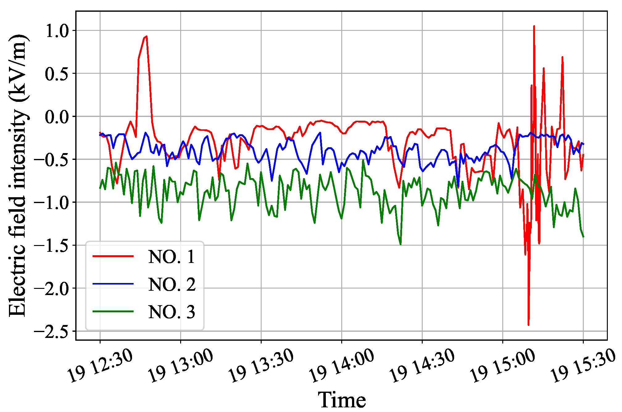
Field mill type atmospheric EF meter is a common device to measure the atmospheric EF, its schematic diagram and physical diagram are shown in Figure 1a,b. It mainly contains a sensing piece and a moving piece, which are similar in shape. Each group of sensing and moving piece has several lobes, like a propeller. When the EF meter is started, the moving piece begins to rotate, and the sensing piece is continuously exposed and obscured with the periodic rotation of the moving piece. The induced currents in the two loops then change with the same value but opposite polarity, and the difference between the two is processed by an operational amplifier and a filter to obtain the raw data. Figure 2 illustrates the measurement data for a three-hour time period at three electric field measurement stations, with a sampling frequency of once per second for a single station.
In the past three years, we have installed about 30 EF measurement stations in Guangzhou city one after another and Figure 1c shows their distribution. In order to facilitate the analysis of lightning in a particular area, Huadu, Baiyun, and Conghua districts are selected as WR.

2.1.2. Lightning Location Data

Lightning is a complex natural phenomenon, the occurrence of lightning is accompanied by electromagnetic signals ranging from very low frequency (VLF) to ultra-high frequency, with the help of which we can use relevant equipment to detect lightning information and thus predict lightning. A lightning locator is a device commonly used to detect lightning, it takes the time difference of lightning VLF electromagnetic pulse arriving at different lightning locators as the basis, and can accurately determine the latitude, longitude, intensity, and polarity of lightning events. Guangzhou Power Supply Bureau, a subsidiary of China Southern Power Grid, which has installed hundreds of lightning locators in Guangdong Province, provided the lightning location data.
A complete multi-station lightning monitoring system consists of four or more lightning locators. Each locator will receive the lightning information and GPS information and transmit it to the central station computer through the communication channel, and then special software is used for time difference positioning calculation, so as to obtain the time, location, intensity, polarity, lightning current, and other parameters of lightning flashes. The lightning locator used in the paper has a temporal resolution less than or equal to 10 7 s and a horizontal spatial resolution less than or equal to 10 m. The system has been tested beforehand and the average positioning error does not exceed 500 m.
According to the analysis of the database, the lightning location data for the whole year 2021 covers almost Guangzhou city, and is widely distributed. Both C-C flashes and C-G flashes will be detected. Note that only C-G lightning location data is used here, as C-C lightning flashes only occur in clouds and have less impact on human activities. In order to correspond to the measurement range of the EF stations in Figure 1c, the data in the upper left of the red dashed line are filtered to further construct the database.

2.1.3. Establishment of Database

For the purpose of discerning whether lightning occurs by EF, it is necessary to intercept a certain length of EF time series to characterize it. If the intercepted series is too long, it will contain a large number of non-thunderstorm EF sequences, and if it is too short, it will reduce the effectiveness of early warning. Generally speaking, the EF changes during the development of thunderstorms can be divided into three stages: thundercloud formation, thundercloud discharge, and thundercloud dissipation. It is worth mentioning that lightning activity is particularly intense in the stage of thundercloud discharge. For most thunderstorms, the time from formation to large-scale discharge is about a few minutes to a few hours.
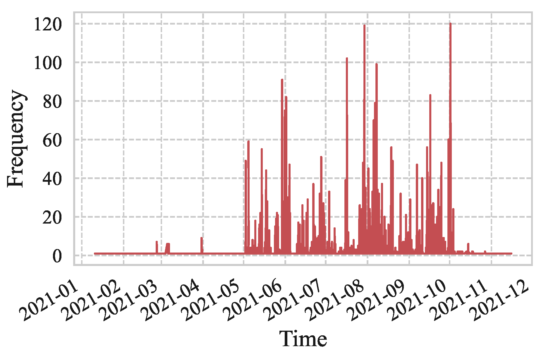
The frequency of lightning strikes for the whole year of 2021 is shown in Figure 3; the statistics are made in a period of one minute (i.e., add up the number of lightning flashes that occurred within 1 min). It can be seen that, for most of the time, the frequency of thunderstorms is about 0, and sometimes the densities of thunderstorms are higher, up to 100 or more. Considering the aggregated nature of lightning occurrences (multiple occurrences within seconds or minutes), if the database is constructed based on each lightning location data, it will result in data redundancy, which is not conducive to the training of the model. Therefore, the 52,267 pieces of data in the database are clustered by 1 min, and if lightning occurs within a certain one-minute time interval, a thunderstorm weather sample can be constructed accordingly.
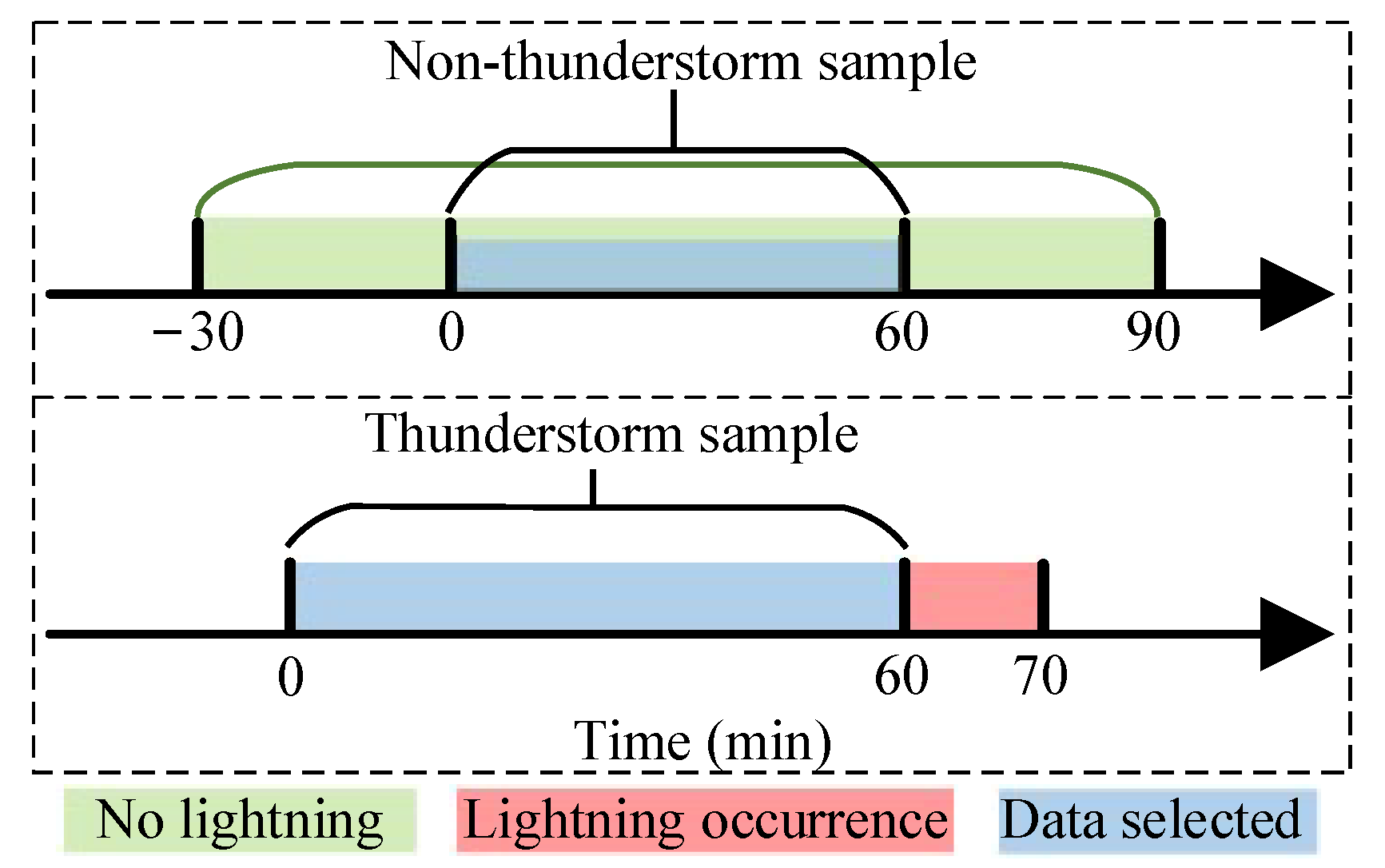
Therefore, in this paper, for thunderstorm weather samples, a 60 min sequence of atmospheric EF is selected, and for non-thunderstorm weather samples, a randomly selected sequence of equal length is taken (shown in Figure 4). The definitions are as follows.
  • Thunderstorm samples: if lightning is monitored within a certain one-minute time interval, the EF measurement data of its past one hour are taken out.
  • Non-thunderstorm sample: randomly take out the EF measurement data for one hour, if there is no lightning occurring before and after half an hour, it is classified as a non-thunderstorm sample, which contains purely sunny days and rainstorms only (no lightning).

2.2. Feature Extraction and Dimensionality Reduction

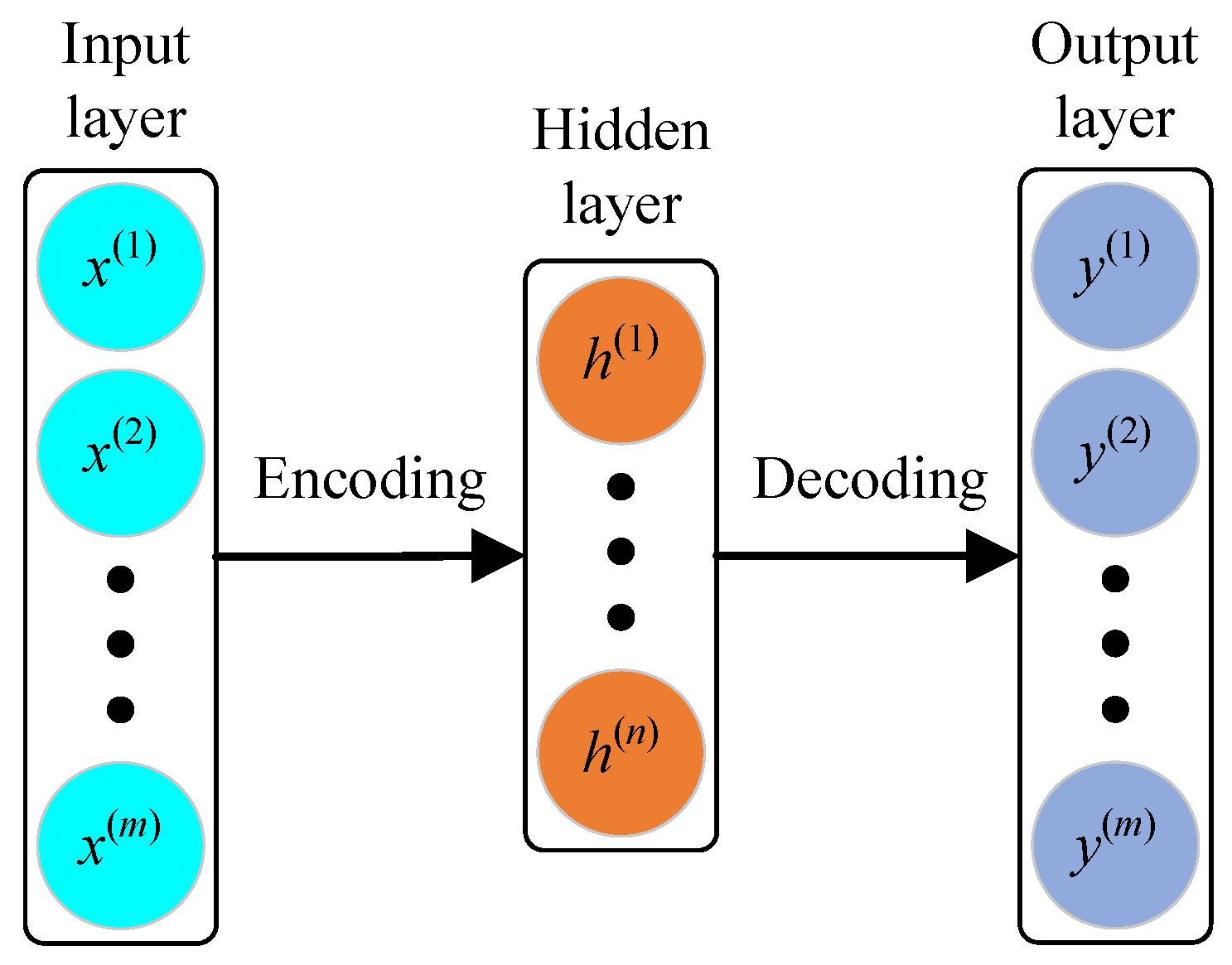
The auto encoder (AE) is one of the most common methods used in machine learning and deep learning to extract features [16,17,18], including a 3-layer structure of input layer, hidden layer, and output layer, and its basic structure is shown in Figure 5. It adopts unsupervised learning and takes the input information as the learning target, which can be used to compress the dimensionality of the input information and is trained by comparing the difference of the original data and the reconstructed data to make the input and output as close as possible, so as to obtain the representation of data in lower dimensions without losing much accuracy [19].
In this paper, SAE is used to extract EF features, whose neurons have a sparse constraint mechanism and the activation function is a sigmoid function ranging from 0 to 1 [20], which can be expressed by the following equation.
σ ( x ) = 1 1 + e x
Suppose X = x 1 , x 2 , , x n 1 , x n ( x i R ( m ) ) is the data sample, where n is the amount of data and m is the dimensionality of features. The encoding network uses the sigmoid activation function to encode the input layer x to obtain the hidden layer h. Then the decoding network decodes the hidden layer to obtain the output vector x ^ . The encoding function f ( x ) and the decoding function g ( h ) are shown in Equations (2) and (3).
h = f ( x ) = f ( W 1 x + b 1 )
x ^ = g ( h ) = g ( W 2 h + b 2 )
where W 1 is the weight from the input layer to the hidden layer, W 2 is the weight from the hidden layer to the output layer, and b 1 and b 2 are the bias terms of the hidden layer and the output layer, respectively.
The core idea of SAE is to introduce a sparse penalty term into the loss function to limit the activation of neurons in the hidden layer. For a given neuron, if its output is close to 1, then its activation level is high. Conversely, its activation level is low if it is close to 0. Let the output of the j-th neuron in the hidden layer be h j ( x ( i ) ) , whose average activity can be denoted as:
ρ ^ j = 1 m i = 1 m h j ( x ( i ) )
where ρ ^ j is the sparsity parameter, and in order to reduce the activation of neurons, whose values are expected to converge to zero, KL scatter is introduced as a penalty term so that ρ ^ j converges to a constant ρ close to zero, and the difference between the two can be expressed in terms of relative entropy as:
KL ( ρ ρ ^ j ) = ρ log ρ ρ ^ j + ( 1 ρ ) log 1 ρ 1 ρ ^ j
The loss function of the AE generally has the form of Equation (6). With the introduction of KL scatter, the loss function of SAE can be expressed by Equation (7).
L = i = 1 m 1 2 x i x ^ i 2
L S A E = L + β j = 1 k KL ( ρ ρ ^ j )
where β is the weighting factor of the sparse penalty term.

2.3. Time Positioning

In order to perform spatio-temporal localization of lightning, the primary problem to be solved is the prediction of lightning occurrence. According to the database established in Section 2.1.3, it is necessary to classify whether lightning occurs or not in the next 1 min based on the measurement data of 30 EF stations. In this section, we will illustrate how to distinguish between thunderstorm and non-thunderstorm weather based on multidimensional EF time series.

2.3.1. Visualization of Electric Field Data

Deep learning has a very wide application in computer vision. Visual image data is two-dimensional data, and the data in the field of lightning warning, which comes from the collection of atmospheric EF data, belongs to a typical one-dimensional time series, thus this problem can be transformed into a time series classification (TSC) problem.
If a one-dimensional array composed of time series is transformed into an image, so that the data from multiple stations are fused together and the characteristics of the atmospheric EF of WR are also available. Further, a deep learning model can be applied to do the analysis, a classification result of whether lightning will occur subsequently can be given.
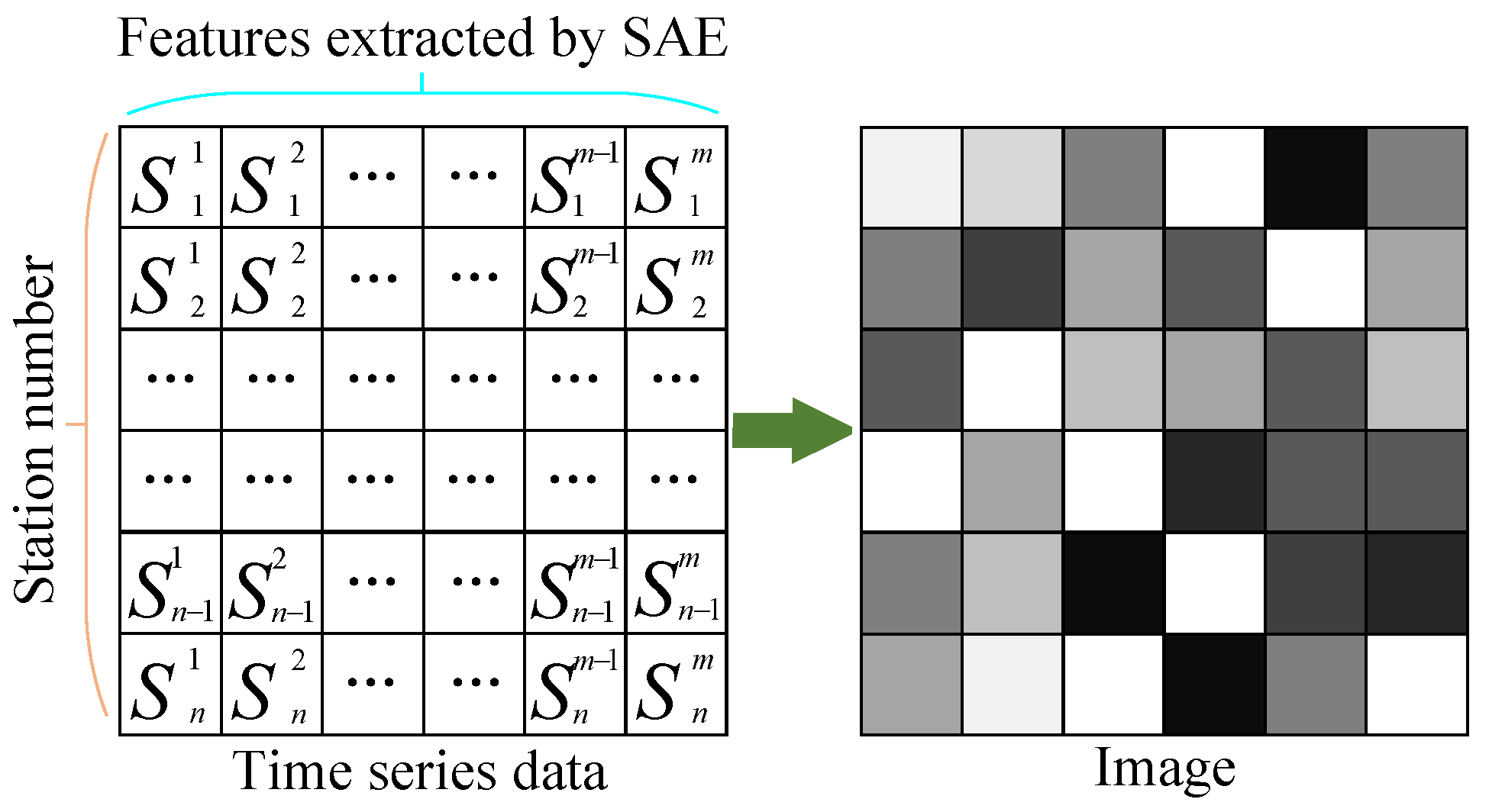
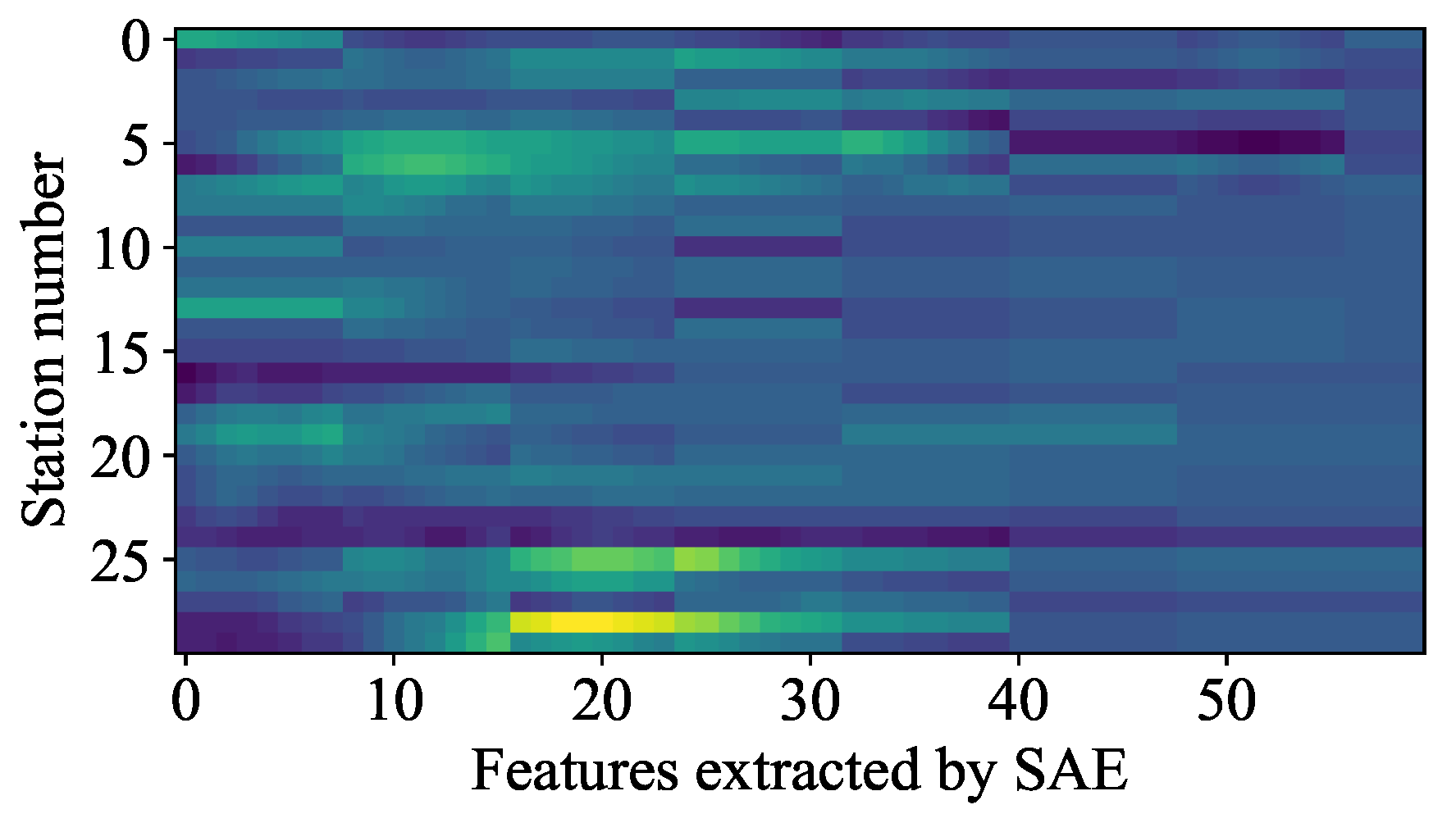
As shown in Figure 6, the visualization of EF data is completed by combining the data of 30 EF stations into one picture, with each row representing the data extracted by SAE from a single station and each column representing the encoded values of 30 stations at a certain moment. Building on the above pre-processing work on the data, we will present an image recognition algorithm next.

2.3.2. ResNet50 Model Architecture

ResNet was proposed in 2015 and won first place on the classification task of the ImageNet competition because of its simplicity and practicality, and many methods have been built on ResNet50 or ResNet101 since then [21,22]. The recognition of weather sample images is more challenging than the recognition of general objects because the weather conditions are complex and variable, the EF station measurements are affected by electromagnetic interference, and the EF images of different thunderstorms present different features. Moreover, thunderstorms occurring out of WR sometimes affect the station measurements to a certain extent, bringing a greater challenge to the classification of weather samples.
The residual structure of ResNet deepens the network structure to facilitate the extraction of deeper features, while effectively solving the problems of gradient disappearance and gradient explosion. It has outstanding achievements in target recognition, image classification and other related fields. Based on the existing weather data samples, taking into account the speed and performance of the model, the ResNet50 network was chosen to classify the weather samples.
As shown in Figure 7, there are 50 layers in the network, including 49 convolutional layers and 1 fully connected layer, which is why it is named ResNet50. The input image size is 224 × 224 and the number of channels is 3. The image data first pass through a convolutional kernel of size 7 × 7 and a max pooling layer, and then the feature information of the images is extracted by stacking multiple layers of residual blocks. Finally, the average pooling layer and the fully connected layer are added, and the probability that the test set images belong to each category is calculated using softmax (Equation (8)) to complete the classification of weather samples.
P G ( x ( i ) ; θ ) = e θ j T x ( i ) l = 1 k e θ l T x ( i )
where θ is the weight parameter, k is the number of categories and P G ( x ( i ) ; θ ) represents the probability that the input sample vector x ( i ) belongs to the j-th classification.

2.3.3. Principle of Residual Block

For the traditional neural network design, one attempts to make the fully trained model more effective in reducing the training error by adding new layers. However, this approach is likely to lead to network degradation, as it is difficult to directly refit the function H ( x ) = x .
To solve this problem, He et al. [23] proposed the concept of residual network in 2015, which can improve the accuracy of the model by adding shortcut branches to deepen the network while avoiding network degradation. The core idea of ResNet is based on the above theory, which can add deeper convolutional layers to improve the model performance. The key role is played by the residual block structure, which effectively prevents the gradient dispersion problem during backpropagation, as shown in Figure 8. At this point, the target to be fitted by the model is no longer the complete output, but rather the difference between the target values H ( x ) and x to achieve identity mapping, which can be expressed by the following equation:
y i = h ( x i ) + F ( x i , ω i )
x i + 1 = f ( y i )
where x i and x i + 1 are the input and output of the i-th residual block, respectively, F represents the residual function, h ( x i ) is the identity mapping, and f represents ReLU activation function.
The features learned from the shallow level l to the deep level L can then be found according to Equations (9) and (10), which is calculated as follows.
x L = x l + i = 1 L 1 F ( x i , ω i )
Then the partial derivative of the loss function with respect to the input can be expressed as
x l = x L · x L x l = x L 1 + x l i = l L 1 F ( x i , ω i )
During the training of the model, x l i = l L 1 F ( x i , ω i ) will not always be −1, i.e., the residual network will not have the problem of gradient disappearance. Meanwhile, x L indicates that the gradient of the deep layer L can be directly passed to the shallow layer l.
Before ResNet was proposed, it was difficult to train very deep neural networks. The proposed structure of residual block ensures that the depth of the network increases without degradation, and the identity mapping allows the network to go deeper and obtain a stronger feature extraction capability.

2.3.4. Improved ResNet50 Network

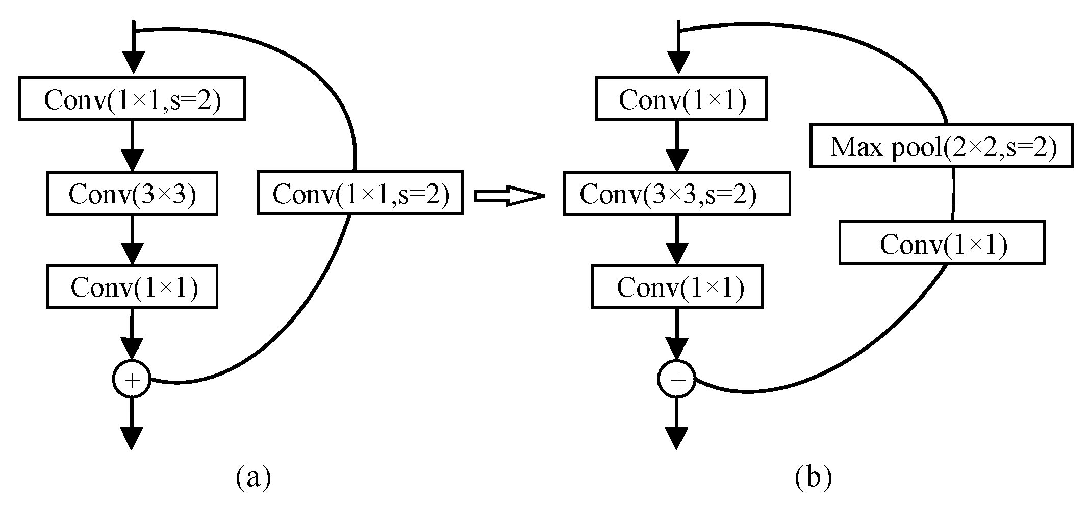
The residual block structure of the standard ResNet50 is shown in Figure 9a. The downsampling is completed by using a 1 × 1 convolutional kernel with a stride of 2 on the shortcut branch and the trunk branch, respectively, but this cannot traverse all the features in the figure, resulting in the loss of some important information, which in turn cannot capture some of the fine features in the timing data and will lead to the degradation of recognition accuracy.
To address the above problem, we shift the down-sampling process of the trunk branch to the 3 × 3 convolution kernel, which allows the residual block to traverse all the information of the weather samples at the beginning and can better extract the features in the EF images. Meanwhile, considering that the EF measurements are usually a few hundred volts per meter on sunny days, whereas in thunderstorms the measurements can reach several thousand volts per meter or even tens of thousands of volts per meter, there is a huge difference between the two. A 2 × 2 maximum pooling layer is added to the shortcut branch, and the maximum pooling operation can extract the maximum value within the pooling window, so as to better distinguish the thunderstorm weather samples from the non-thunderstorm weather samples.
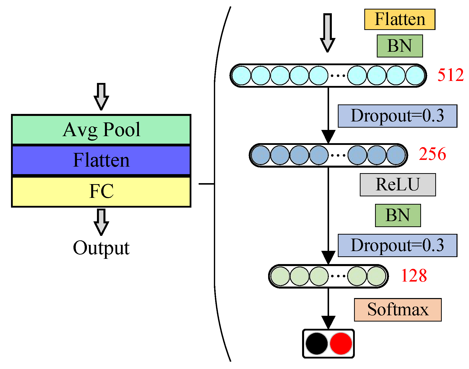
In addition, the ResNet50 network needs to be fine-tuned, i.e., the pooling and fully connected layers in the tail are replaced to make it more suitable for the binary classification task of weather samples in this paper. The fine-tuned network is shown in Figure 10, where the previous image data is flattened into one-dimensional data and then compressed in a series of operations to obtain the probability distribution of the two types of weather samples via the softamx equation. The BatchNorm operation [24] helps to improve the speed of model training and can effectively avoid gradient disappearance and explosion, and the Dropout operation can improve the generalization ability of the model.

2.4. Spatial Positioning

After finishing the classification of the EF time series data according to the above algorithm, we can clearly know whether lightning will occur in the next minute. It is followed by another algorithm that we propose, which helps to judge the possible location of lightning by the EF measurement data.

2.4.1. Spatial Correlation of Lightning

Several samples of thunderstorms are listed in Figure 11, where the colored dots represent lightning that occurred during the corresponding time period and the pink rectangular area represents the lightning’s gathering area. In the exploration of the lightning location data, the following rules were found:
  • A single thunderstorm is often accompanied by multiple lightning episodes.
  • As shown in the pink rectangle in Figure 11, lightning flashes that occur within a few minutes have obvious spatial correlation characteristics.
When a thunderstorm cloud forms at a certain location, it creates a massive discharge phenomenon in the area. The above patterns suggest that there is indeed some spatial connection in the location of lightning occurrence.
Given a finite set of points x 1 , x 2 , , x k R n , their geometric center C is defined as:
C = x 1 + x 2 + + x k k
According to Equation (13), combined with the weather sample database in Section 2.1.3, we intend to construct the correlation between the EF data and the lightning occurrence location by equating the latitude and longitude coordinates of lightning occurring every minute into a point. Therefore, the task of this section is to infer the equivalent centers of all flashes occurring in one minute from EF measurements of 30 stations. A lightning strike on an electrical facility could cause a regional power outage, while a lightning strike on a critical communication line could bring about a communication disruption. Once we know the possible areas of lightning and take measures in advance, the damage caused by lightning can be reduced to a large extent.
Nowadays, scholars of thunderstorm electricity usually attribute thunderstorms to multiple charge structures [25]. Coulomb’s law describes the quantitative relationship between electric charge and electric field. Nevertheless, in real life the situation can be more complicated, which motivates us to propose a method to construct a reasonable inference of the lightning occurrence location given by the measured values of 30 stations.

2.4.2. Multilayer Perceptron

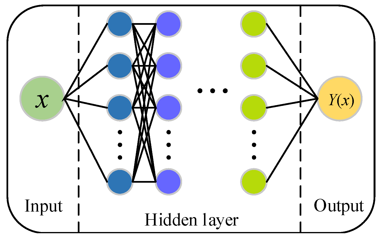
Multilayer perceptron (MLP) was a popular machine learning method in the 1980s with a wide range of applications, such as speech recognition, image recognition, machine translation, etc. [26,27,28]. However, since the 1990s, MLP has encountered strong competition from support vector machines (SVM). In recent years, MLP has gained renewed attention due to breakthroughs in deep learning. Figure 12 illustrates an MLP network structure containing an input layer, a hidden layer, and an output layer. As shown in the figure, the compression encoding of the dataset is obtained by nonlinearly mapping the input dataset to the hidden layer, i.e., the feature information of the original data in another dimensional space is obtained, which is sufficient to characterize the information of the input layer. Thus, the purpose of reducing the data dimension and improving the computational efficiency can be achieved. Theoretically, it is possible to approximate the nonlinear mapping relationship with arbitrary accuracy by including enough hidden layers and neuron nodes.
In order to explore the correlation between the lightning location and EF data, an MLP model is designed in this paper, as shown in Figure 13. MLP is suitable for solving problems such as classification and prediction as it is capable of fitting complex non-linear functional relationships with high adaptability, self-learning, and fault tolerance. The number of nodes in the input layer is related to the dimensionality of the input data, and the same applies to the output layer. The hidden layer can have multiple layers, each of which can be configured with any number of nodes. The number of nodes and type of each layer affect the performance of the entire network and can be changed according to practical needs. On the one hand, if the model is too simple, the relationship between input and output cannot be well constructed, which will lead to large training errors. On the other hand, overly complex models can cause training and prediction to consume a lot of time, which can neither validate the idea and improve the model quickly, nor achieve fast prediction, and will easily lead to overfitting. In Section 3.3, we will test and further analyze the performance of the space positioning module.

2.5. Overview of the Proposed Algorithm

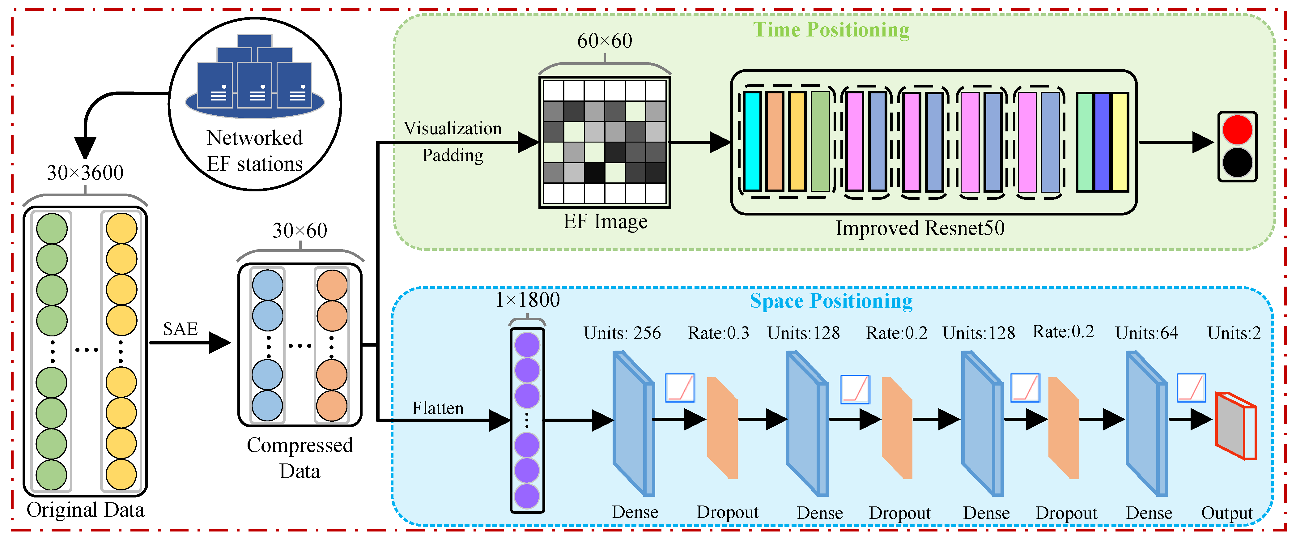
The structure of lightning warning system can be divided into two parts. First, the features extracted by a SAE are transformed into an image to conclude whether it is a thunderstorm weather or not based on the improved ResNet50. Finally, if the above weather sample is determined to be a thunderstorm weather, the lightning spatial localization is initiated and the latitude and longitude of lightning occurrence is predicted based on the MLP neural network proposed in this paper. The overall structure of the algorithm is shown in Figure 13, which is mainly summarized as the following steps:
  • Data collected from 30 EF stations and lightning locators are pre-processed.
  • The EF measurement data and lightning location data are matched one by one to construct the database of weather samples.
  • The characterization of the EF time series is extracted by a SAE.
  • EF features extracted in the previous step are transformed into images and determined whether they are thunderstorm weather samples based on the improved ResNet50 network. If yes, the process proceeds to the next step; otherwise, the process is finished.
  • Lightning spatial localization is initiated and the latitude and longitude of the lightning occurrence is predicted based on a MLP neural network.

3. Results

The experimental environment includes: Memory: 32 G; CPU: Intel Core i9-10900K; GPU: RTX3080; System: Windows 10 Professional 64-bit. The pytorch deep learning framework was used, and the experiments were conducted in Python 3.8.8.

3.1. Feature Extraction

For a single EF station, since its sampling frequency is 1Hz, 3600 samples of data can be collected in one hour. The dimensionality of a single weather sample can reach 3600 × 30, which is not conducive to the model for fast computation. The dimensionality of data from one station is compressed from 3600 to 60 using a SAE, and the dimensionality of the weather samples is thus reduced to 60 × 30. Mean square error (MSE) is used as the evaluation index for model training, and the formula is defined as follows.
M S E = 1 m i = 1 m ( y i y ^ i ) 2
where m is the sample size, y i is the original data, and y ^ i is the reconstructed data.
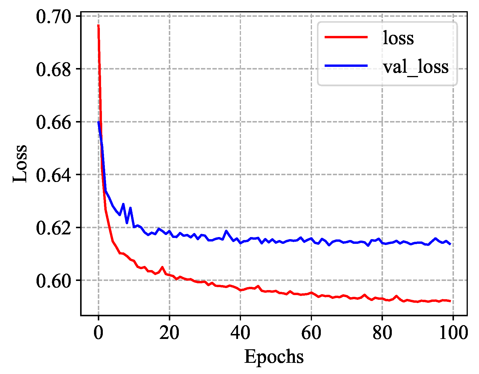
According to the formula in Section 2.2, ρ is set to 0.05, β is set to 3, the batchsize is set to 16 to speed up the operation, 80% of the weather samples are used as the training set and the remaining 20% as the validation set. The SAE network was continuously trained through 100 epochs, and the result is shown in Figure 14.
As can be seen from the figure, with the increasing number of iterations, the gap between the original data and the compressed data keeps decreasing. The MSE of the validation set finally stabilized below 0.62, indicating that the data processed by the SAE can effectively express the features of the original data.

3.2. Time Positioning

By mapping one to one with the RGB color table, the transformation from multiple sets of one-dimensional EF data to images can be realized, thus making it possible to fuse data from multiple stations with the ability to express EF information within the WR. First, the data needs to be normalized according to Equation (15). Then, the normalized values E s are mapped to the (0–255) interval according to Equation (16), and a grayscale map with a specification of 60 × 30 is obtained. The padding operation fills in the gaps at the top and bottom of the image so that the core information is in the middle, thus changing the image size to 60 × 60.
E s = E E min E max E min
C = E s × 255
where E represents the original EF data before conversion, and E min and E max represent the minimum and maximum values of the measured data, respectively.

3.2.1. Classification Result

According to the database created in Section 2.1.3, with a total of 10,093 weather samples, of which 4665 are thunderstorms and 5428 are non-thunderstorms. The training and validation sets are divided according to the ratio of 9:1. The thunderstorm samples and non-thunderstorm samples are classified using the model proposed in Section 2.3. The negative log likelihood (NLL) loss is used, which is useful to train a classification problem with C classes. Its specific expression is as follows.
l o s s = 1 m i = 1 m y log P G ( x ( i ) ; θ )
where m is the sample size, y represents the target value, which is the true category of weather samples, P G ( x ( i ) ; θ ) is the softmax function, which can be calculated using Equation (8).
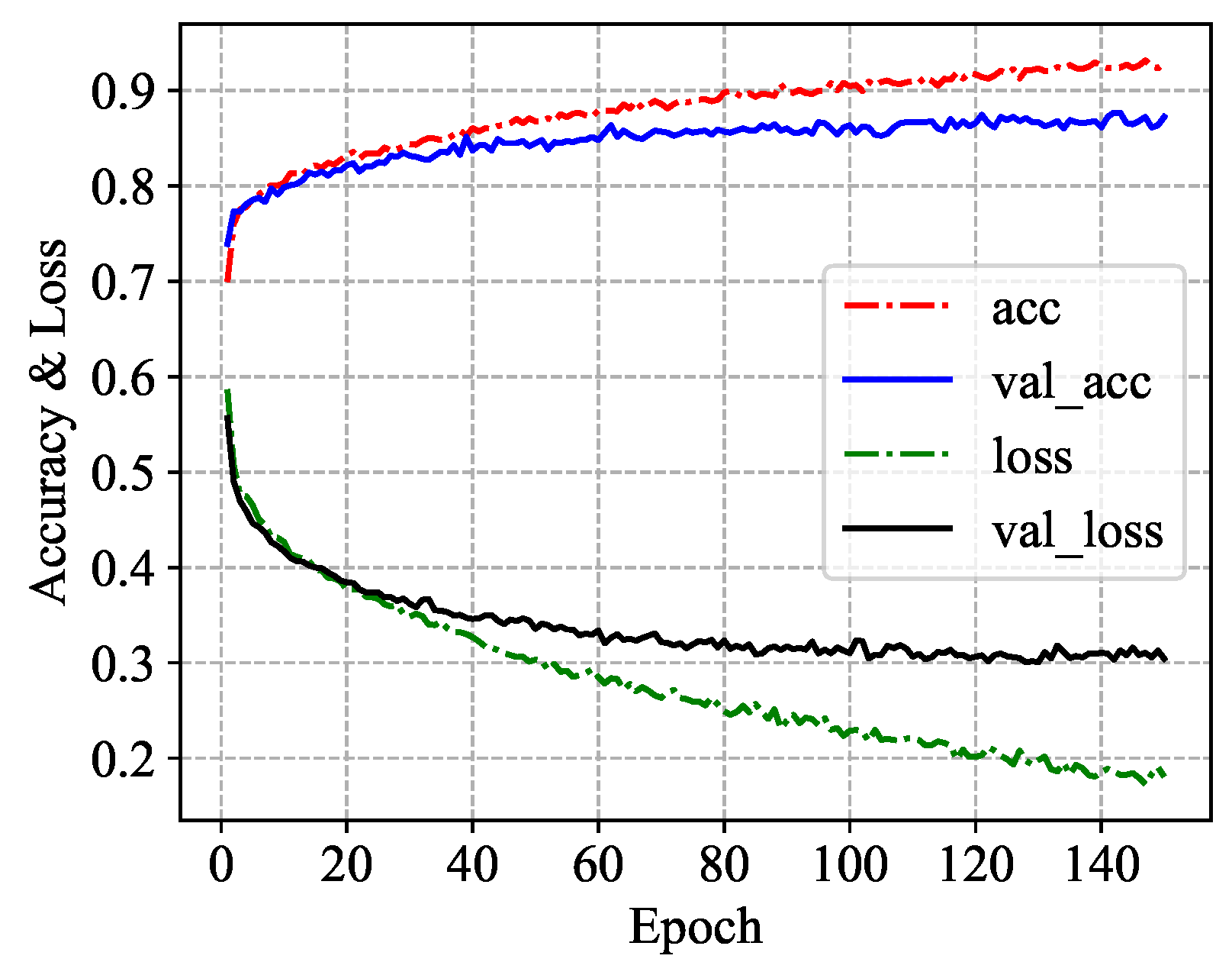
The learning rate was set to 0.005 and the parameters were updated iteratively using stochastic gradient descent (SGD). Figure 15 shows the changes of accuracy and loss function during the training process for the training and validation sets, respectively. Obviously, after 150 epochs of training, the accuracy of the training set and the validation set are stable at about 92% and 87%, and the difference between them is small, which indicates that the model has not overfitted and achieves a good recognition of thunderstorm samples and non-thunderstorm samples. The loss of validation set was held constant starting at around 120 epochs, and the model reached stability. In summary, the model shows excellent performance for the dichotomous task of thunderstorm weather and non-thunderstorm weather.

3.2.2. Evaluation for Different Length of Time Series

The length of the EF time series input to the model also has a significant impact on the accuracy of the model. If the selected sequence is too long, it will contain a large number of non-thunderstorm sequences while increasing the computation time. If it is too short, the accuracy of the model will be affected. In the previous section, we conducted experiments on a 60 min EF time series. Therefore, in this section, the EF time series of 30, 35, 40, 45, 50, and 55 min before the occurrence of lightning are selected as the input of the model to investigate the effect of the length of EF time series on the accuracy of the model.
In the field of machine learning, for binary classification problems, the results can be classified into four cases: true positive examples, false positive examples, true negative examples, and false negative examples, according to the combination of the true category and the prediction results. The joint table of the predicted and true results is shown in Table 1.
On the basis of the results in Table 1, the following four metrics are defined in order to evaluate the performance of the model.
Accuracy = T P + T N T P + T N + F N + F P
Precision = T P T P + F P
Recall = T P T P + F N
F 1 = 2 P R P + R
In Equations (18)–(21), P stands for Precision and R stands for Recall; Accuracy represents the proportion of correctly predicted samples to all samples; Precision represents the proportion of samples currently predicted to be positive that are correctly classified (i.e., the proportion of true positive samples); Recall represents the proportion of true positive samples among those positive samples; F 1 score is the weighted summed average of Precision and Recall, which is set to measure Precision and Recall together.
Table 2 shows the results obtained for time series of different lengths in the validation set (908 weather samples), from which it can be seen that the scores of the four indicators show an increasing trend as the length of the time series increases. The best results can be achieved with the 60 min time series. The reason may be that, for samples of thunderstorms, which often last for more than several hours [29,30], the longer the time series is, the richer the amount of information it contains, which is conducive to the model to make the judgment of whether a thunderstorm will occur. Considering the need to make short-time proximity forecasts and the limited computational performance, time-series data of up to 1 h are selected for the experiments in this paper.

3.2.3. Evaluation under Data Augmentation

In practical applications, training neural networks often encounters the problem of insufficient data. Consequently, in order to get more data, some small changes need to be made to the existing image dataset, such as rotating, panning, and stretching, and the network will consider it a different image. Nevertheless, it is important to note that the strategy of data enhancement is not chosen arbitrarily. In this paper, it involves the identification of EF data from multiple stations, so if operations such as rotating and cropping are performed on them, the correspondence between EF and lightning will be destroyed. In order to expand the amount of data and enrich the amount of information expressed in the images, shown in Figure 16 is a visualization of a weather sample. For the training set images, the position of each row of EF data is randomly swapped. For the validation set images, no changes are made.
Table 3 shows the changes of the four evaluation metrics before and after data augmentation (Aug stands for augmentation), and the performance comparison with other methods. Despite the fact that the “Precision” does not change much, the “Recall”, “ F 1 ”, and “Accuracy” of the model are improved to a large extent. In addition, it is clear that the results of the improved network show an enhancement in the performance of the four metrics compared with the original ResNet50 (where the residual block was not improved). Compared to the convolutional neural network (CNN), and a common temporal data processing algorithm long short-term memory (LSTM) and metrics in other literature, the improved ResNet50 proposed in this article has shown superior performance. The advantage of transfer learning is that it can quickly produce a desired result based on a pre-trained model and provide excellent capabilities when the data set is small. According to the above experimental results and analysis, it is obvious that data augmentation can further improve the accuracy and enhance the generalization ability of the model.

3.2.4. Effect of Noise Interference

Robustness is an important evaluation index of deep learning models, and it is mainly used to check whether the model can maintain the accuracy of judgment in the face of small changes in the input data, i.e., whether the model performs stably in case of certain changes. The level of robustness directly determines the generalization ability of deep learning models. Generally speaking, the more accurate the model is, the less robust it is in general.
In real-world application scenarios, the data to be processed contains more heterogeneous variations. In this paper, the measurement of atmospheric EF is affected by the surrounding electromagnetic environment, even though we have taken this into account when installing the equipment and pre-processed the EF data. It is still not possible to completely eliminate the effects of electromagnetic interference, so robustness testing is necessary. Signal-to-noise ratio (SNR) is a common metric used in science and engineering to compare the strength of the desired signal with the strength of the background noise, with the basic meaning of the ratio of useful signal power P s to noise power P n .
S N R = 10 lg P s P n
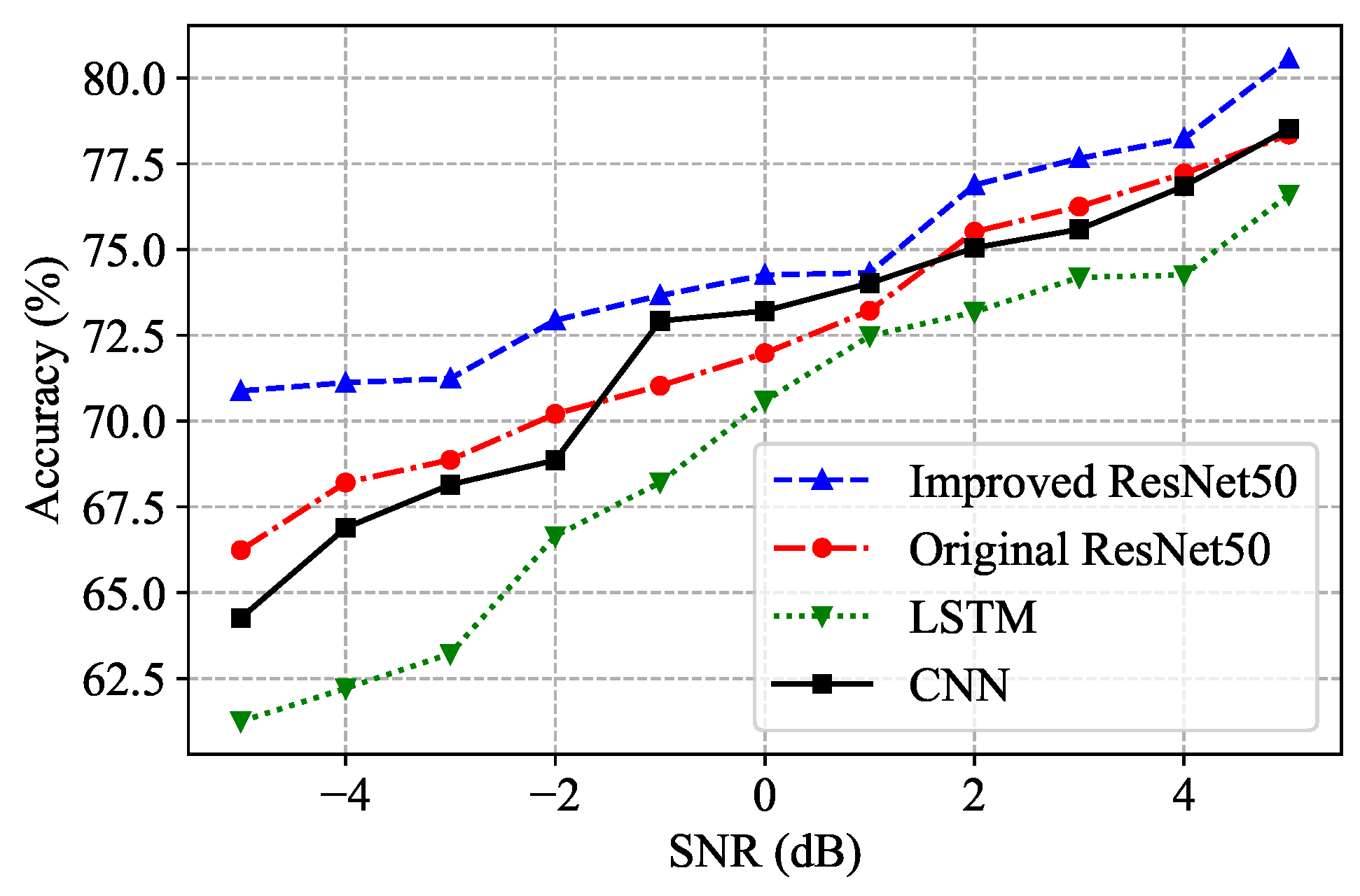
Robustness tests are conducted based on several other common classification algorithms and the improved ResNet50. No noise is added to training set and white noise with standard normal distribution is added to validation set. The results are shown in Figure 17. It is worth mentioning that, with the increase of SNR, the accuracy of all five models has been improved to some extent, but the improved model based on ResNet50 proposed in this paper still performs best, and the accuracy of the model can be kept at a high level with a strong robustness under the interference of a certain degree of noise. However, the other three common algorithms are less resistant to noise. In particular, the LSTM algorithm shows large fluctuations in accuracy after adding noise to the original electric field time series. In summary, the improved ResNet50 model has superior robustness.

3.3. Spatial Positioning

Determining the spatial location of lightning occurrence is the second step of lightning spatio-temporal localization. In Section 3.2, we were able to determine whether a thunderstorm weather will occur. Next, another method is needed to determine the specific location of lightning occurrence. Once we know the possible areas of lightning, and when a thunderstorm is approaching, lightning warning instructions can be issued in advance, so that active lightning protection measures (such as blocking the lightning surge intrusion channel and artificial triggered lightning) can be taken in relevant areas, thereby reducing or avoiding the safety hazards caused by lightning [33,34].

3.3.1. Performance of Lightning Localization

In Section 2.4.2, we constructed a MLP model, which now needs to be trained and experimented on. The MSE (Equation (14)) is used as the loss function to train the network. The MAE is used as the evaluation metric and is defined as follows.
M A E = i = 1 n y i y ^ i
The ReLU nonlinear activation function of the neurons in the middle hidden layer is chosen, which can avoid the gradient disappearance and gradient explosion caused during network training. Using the error back propagation (BP) algorithm to update the weight and bias of each neuron, the training process can be expressed as Equations (24)–(28).
E k = 1 2 j n ( y ^ j k y j k ) 2
Δ w h j = α E k w h j
Δ b h = α E k b h
w h j = w h j + Δ w h j
b h = b h + Δ b h
For a given k-th training sample ( x k , y k ) , we use Equation (24) where y ^ j k represents the output value of the j-th neuron and y j k is the corresponding label value. E k represents the MSE of the k-th training sample and α is the learning rate. After calculating the gradient of the neuron parameters by Equations (25) and (26), the weights and bias of the layer can be updated by Equations (27) and (28) to make the network parameters move in the direction of a smaller MSE. In order to avoid overfitting and falling into local optima during network training, a Dropout layer can be introduced to discard the values of partial neurons. The initial learning rate was set to 0.001 and Adam was used as the optimizer for the training of the above neural network model.
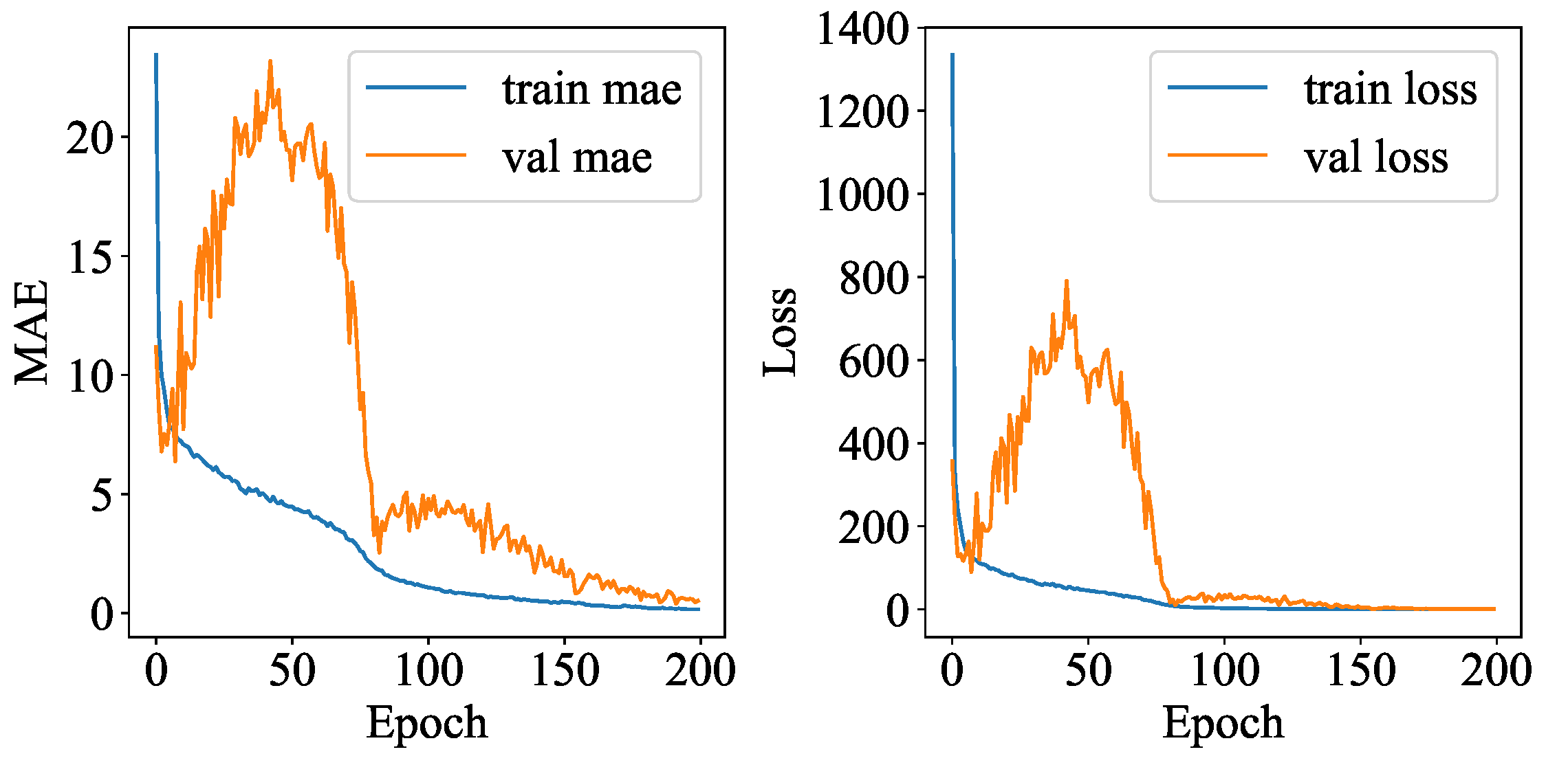
Figure 18 displays the results of training and validation sets, from which it can be seen that with the continuous iterative training of the network, the MAE and MSE continue to decrease. As the EF data has been initially extracted by the SAE, the shortage of manual feature extraction is avoided. After obtaining a representation of the raw data in a low dimension, the MLP network is used to construct its correlation with the latitude and longitude of the lightning occurrence, with the aim of constructing a non-linear relationship. In this case, it is possible to achieve satisfactory results without designing an overly complex network model. The MAE and loss for validation set finally stabilized at 0.82 and 0.89.
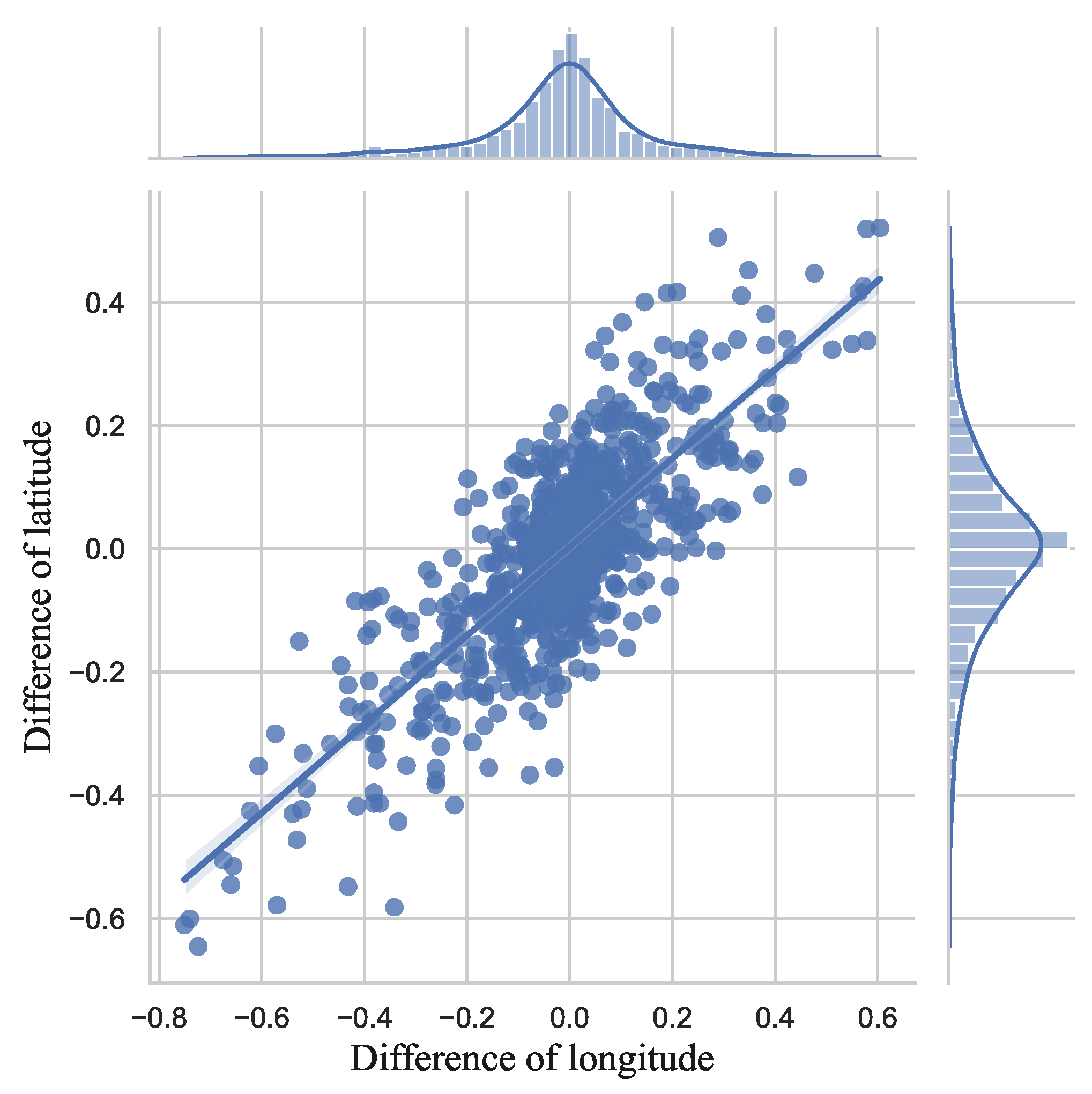
Figure 19 is a scatter plot with histograms of the real latitude and longitude and predicted latitude and longitude of thunderstorm weather samples in validation set. Each point represents the difference between the predicted and actual values of latitude and longitude for a given sample, and the closer to the origin (0, 0), the smaller the error is and the more accurate the lightning is located. The latitude and longitude sent to the network for training are normalized beforehand to eliminate the influence of the magnitude between the data, and the straight line in the graph represents the regression line of the difference in longitude and the difference in latitude (with slope close to 1). Through two histograms, it can be clearly seen that for most of the thunderstorm samples, the model performs well for lightning center localization, with longitude error controlled within ±0.25 and latitude error controlled within ±0.2.

3.3.2. Evaluation for Different Length of Time Series

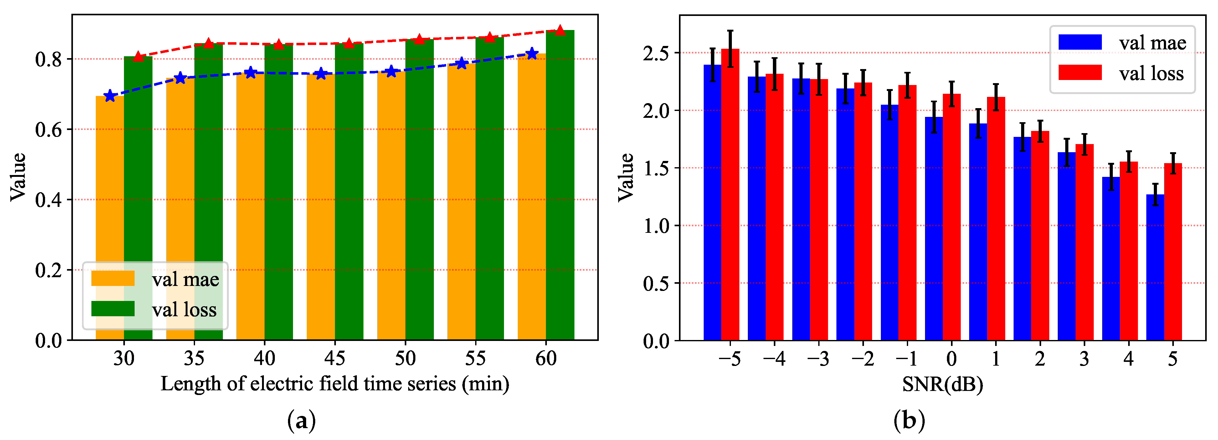
In this section, we will explore the effect of different lengths of EF time series on the spatial localization of lightning. The performance of space positioning module will be further investigated. For different lengths of time series, the variations in the MAE and loss of the validation set need to be observed, and the results after the model has been trained and reached stability are shown in Figure 20a. All experiments were repeated five times for averaging to avoid the factor of chance. By varying the length of the time series used for model training and exploring the changes in loss and MAE of the validation set, no significant effect of the length of time series on the accuracy of lightning spatial localization was found. It is worth noting that as the length of the time series increases, the values of MAE and loss also show an upward trend, but the changes are not significant. Combined with the relationship between the EF and the thundercloud charge, it can be reasonably inferred that it is strictly feasible to locate lightning using EF measurements at a specific time, and an increase in the length of the time series does not imply an increase in accuracy, on the contrary, is likely to lead to an increase in error.

3.3.3. Effect of Noise Interference

As described in Section 3.2.4, the robustness of the model must also be considered. Similarly, a 60 min time series was used and a percentage of the noise signal was added to the original EF data of the validation set.
Figure 20b displays the variation of MAE and loss of the space positioning module under noise disturbance. In general, compared to the results in Section 3.3.2, both MAE and loss increased to varying degrees with the addition of noise, proportional to the noise intensity, implying that noise can indeed interfere with lightning spatial localization to some extent. As the dropout layer is introduced, it can discard some values in the hidden layer with a certain probability, thus significantly reducing the overfitting phenomenon and making it exhibit better robustness in the face of noise interference. Overall, the variation in positioning results is within acceptable limits.
To summarize, the length of the sequence fed into the MLP model shows no obvious pattern and has little effect on the accuracy. Meanwhile, it presents strong robustness against noise interference. Following immediately, we will list three real-world cases during the operation of the lightning warning system whose performance will be further analyzed.

4. Discussion

The construction of lightning warning system is basically completed after the above methods passed the accuracy and robustness tests. The following are a few case studies of the actual operation of the model. These three cases are three presentations of the complete life cycle of thunderstorms. Since the lightning flashes are too intensive to be easily read if they are all put in one figure, a complete life cycle of a thunderstorm is divided into three figures for display, which can better reveal the prediction performance and the pattern of thunderstorm evolution.
As shown in Figure 21a, Case 1 is a thunderstorm that occurred on 2 May 2021 from 13:37 to 14:07. The model can first give a judgment whether there will be flashes based on the electric field measurements in the past hour, and then the location of the lightning center. Table 4 shows the calculated results given by the system per minute and the comparison with the real values. According to Equation (13), the points of all lightning flashes are equated to a point called the geometric center (blue numbers in Figure 21), and the location that the system predicts lightning to occur is called the prediction point (red numbers in Figure 21). It is worth noting that that lightning may not occur every minute, nor does the system make the determination that there will be lightning each minute. As described in Table 1, there will be four cases (TP, FP, FN, TN) based on the predicted values and the actual observations. In this example, 13:37 is taken as the first minute of the start and the number of lightning flashes that occurred during each minute is given. The geometric center, the predicted point and the distance between the two are also listed. For example, in the first minute (13:37) there were two lightning flashes detected, the geometric center is (113.37, 23.51), and the predicted point is (113.32, 23.41), and the distance between them can be calculated by the following equation.
S = 2 R arcsin sin 2 a 2 + cos ( l a 1 ) × cos ( l a 2 ) × sin 2 b 2
where a and b are the difference in longitude and latitude of the two points, respectively; l a 1 and l a 2 represent the latitudes of the two points; R is the radius of the Earth, which is about 6378 km.
According to Equation (29), the distance between the prediction point and geometric center at 13:37 is about 12.65 km, indicating that the system does indicate the approximate location of lightning flashes. At the same time, from the whole thunderstorm process, the accuracy of the prediction declined for the small number of flashes with more scattered distribution (“1”, “3” in Figure 21a), which may be due to the low charge of the thunderstorm clouds and the relatively weak discharge phenomenon, resulting in the electric field meter not detecting the intense fluctuation changes. However, normally, the horizontal range of a single thunderstorm is about a few kilometers to 20 km [35], and the average motion speed of a thunderstorm is 13.22 m/s [36]. The model proposed in this paper is able to give predictions at every minute, which means that the location and motion of discharge areas can be inferred from the predictions made a few minutes before and after. As can be seen from Table 4, the distance between the predicted points and the geometric centers are mostly in the range of 5–15 km. Combined with Figure 21a, even if the model’s prediction deviates widely at a certain moment, it is still possible to know the area where lightning will occur by subsequent predictions.
Case 2 occurred on 10 June 2021 from 15:29 to 15:59. As shown in Figure 21b, it can be clearly seen that the flashes were more concentrated. From 15:29 to 15:41, the number “1” represents the lightning occurred in the first minute. From Table 5, we know that only two flashes occurred, and the distance between the predicted point and the geometric center is 16.9 km. However, during the periods of 15:42–15:51 and 15:52–15:59, most of the subsequent flashes were found to be concentrated in the square area of longitude (113.2, 113.3) and latitude (23.3, 23.5). From the spatio-temporal localization results, it is obvious that the model is able to locate lightning flashes, and a relatively large locational error at a given moment does not affect the overall determination of the massive discharge area.
Presented in Figure 21c, Case 3 was recorded on 17 August 2021 from 18:32 to 19:02. At 18:32–18:43, the distribution of lightning was more scattered, but was mainly found in the northeastern part of the Conghua district. However, the subsequent lightning events were more concentrated (18:44–18:53), when there may have been a merger of multiple thunderstorm clouds [37,38,39]. In addition, as can be seen from Table 6, at this time the thunderstorm weather was particularly intense, with up to 45 lightning flashes per minute. Finally, at 18:54–19:02, the distribution of lightning was more dispersed, implying that the thunderstorm clouds started to develop toward the dissipation process. Thus, the algorithm proposed in this paper can not only locate lightning in time and space, but can also judge the process of lightning formation, development and dissipation based on the results of multiple warnings, which is of great significance for grasping the mechanism of thunderstorms and lightning protection.
Sometimes, during the development of a thunderstorm, ice crystals, shrapnel, and other particles in the clouds are constantly charged by friction, resulting in a strong electric field between the atmosphere and the ground. Although the electric field meter detects a strong electric field at this time and predicts that lightning will occur next, no lightning actually occurs at this time. However, this is usually reflected in the actual observations over the next few minutes. Similarly, when lightning occurs, the charge in the clouds is released, so the electric field measured on the ground drops accordingly, which may cause the model to give a result of no lightning occurring. However, in general, as shown in Table 3, the model is able to maintain an accuracy of more than 80%.

5. Conclusions

In this paper, a deep learning framework for lightning prediction is proposed. First, the features of the original EF time series data are extracted using a SAE. Then, the above extracted features are used to construct a visual picture of EF measurement data of multiple stations. Next, the weather samples are classified based on the improved ResNet50 model to conclude whether a thunderstorm will occur in the next one minute. Finally, if it is judged that lightning will occur in the future, the center of lightning flashes is predicted based on the MLP model. In practice, the model can determine the trend of lightning with multiple predictions made in a few minutes, while also improving fault tolerance.
The composition of lightning prediction model is divided into two parts, i.e., making predictions about the time and location of lightning occurrence, which were tested for accuracy and robustness respectively. Due to the chaotic nature of lightning, it is challenging to forecast it. Taking into account the computational cost and prediction accuracy, more reliable lightning spatio-temporal localization results are given and analyzed with practical cases. The experimental results show that the proposed model has statistically quite high prediction capability for short-time proximity warning, which helps to improve the lightning protection level in the region, and active lightning protection measures can be taken to further reduce the property and safety losses caused by lightning according to the relevant results.

Author Contributions

Conceptualization, Y.Z., B.J.M. and Z.Z.; data curation, R.B. and Y.Z.; methodology, R.B. and Z.Z.; resources, Z.H.; writing—original draft preparation, R.B.; writing—review and editing, R.B., Y.Z. and B.J.M. All authors have read and agreed to the published version of the manuscript.

Funding

This research was funded by the science and technology project of China Southern Power Grid Limited Liability Company (Project No. GZHKJXM20170061).

Institutional Review Board Statement

Not applicable.

Informed Consent Statement

Not applicable.

Data Availability Statement

The data reported in this article is available from the authors upon request.

Acknowledgments

We thank the Guangzhou Power Supply Bureau of China Southern Power Grid for providing the data required in the paper. We are also grateful to three anonymous reviewers for their helpful comments, which significantly improved the quality of our paper.

Conflicts of Interest

The authors declare no conflict of interest.

References

  1. Qie, X.; Liu, D.; Sun, Z. Recent advances in research of lightning meteorology. J. Meteorol. Res. 2014, 28, 983–1002. [Google Scholar] [CrossRef]
  2. Yu, X.; Zheng, Y. Advances in severe convection research and operation in China. J. Meteorol. Res. 2020, 34, 189–217. [Google Scholar] [CrossRef]
  3. Ivanova, A. International practices of thunderstorm nowcasting. Russ. Meteorol. Hydrol. 2019, 44, 756–763. [Google Scholar] [CrossRef]
  4. Bala, K.; Choubey, D.K.; Paul, S. Soft computing and data mining techniques for thunderstorms and lightning prediction: A survey. In Proceedings of the 2017 International conference of Electronics, Communication and Aerospace Technology (ICECA), Coimbatore, India, 20–22 April 2017; Volume 1, pp. 42–46. [Google Scholar]
  5. Hayward, L.; Whitworth, M.; Pepin, N.; Dorling, S. A comprehensive review of datasets and methodologies employed to produce thunderstorm climatologies. Nat. Hazards Earth Syst. Sci. 2020, 20, 2463–2482. [Google Scholar] [CrossRef]
  6. Moon, S.H.; Kim, Y.H. Forecasting lightning around the Korean Peninsula by postprocessing ECMWF data using SVMs and undersampling. Atmos. Res. 2020, 243, 105026. [Google Scholar] [CrossRef]
  7. Mostajabi, A.; Finney, D.L.; Rubinstein, M.; Rachidi, F. Nowcasting lightning occurrence from commonly available meteorological parameters using machine learning techniques. Npj Clim. Atmos. Sci. 2019, 2, 1–15. [Google Scholar] [CrossRef]
  8. Gharaylou, M.; Pegahfar, N.; Farahani, M.M. Influence of tilting effect on charge structure and lightning flash density in two different convective environments. Meteorol. Appl. 2020, 27, e1957. [Google Scholar] [CrossRef]
  9. Yang, B.; Gao, X.; Han, Y.; Zhang, Y.; Gao, T. A thunderstorm identification method combining the area of graupel distribution region and weather radar reflectivity. Earth Space Sci. 2020, 7, e2019EA000733. [Google Scholar] [CrossRef]
  10. Bao, R.; He, Z.; Zhang, Z. Application of lightning spatio-temporal localization method based on deep LSTM and interpolation. Measurement 2022, 189, 110549. [Google Scholar] [CrossRef]
  11. Zhang, Y.; Li, H.; Wang, Z.; Zhang, W.; Li, J. A preliminary study on time series forecast of fair-weather atmospheric electric field with WT-LSSVM method. J. Electrost. 2015, 75, 85–89. [Google Scholar] [CrossRef]
  12. Xing, H.; Yang, X.; Zhang, J. Thunderstorm cloud localization algorithm and performance analysis of a three-dimensional atmospheric electric field apparatus. J. Electr. Eng. Technol. 2019, 14, 2487–2495. [Google Scholar] [CrossRef]
  13. Wang, G.; Kim, W.H.; Kil, G.S.; Park, D.W.; Kim, S.W. An intelligent lightning warning system based on electromagnetic field and neural network. Energies 2019, 12, 1275. [Google Scholar] [CrossRef] [Green Version]
  14. Adzhieva, A.A.; Shapovalov, V.A.; Mashukov, I.K. Local sensing of atmospheric electric field around Nalchik City. In Proceedings of the Advanced Environmental, Chemical, and Biological Sensing Technologies XIV, Anaheim, CA, USA, 9–10 April 2017; Volume 10215, p. 102150W. [Google Scholar]
  15. Srivastava, A.; Mishra, M.; Kumar, M. Lightning alarm system using stochastic modelling. Nat. Hazards 2015, 75, 1–11. [Google Scholar] [CrossRef]
  16. Wang, Y.; Yao, H.; Zhao, S. Auto-encoder based dimensionality reduction. Neurocomputing 2016, 184, 232–242. [Google Scholar] [CrossRef]
  17. Lange, S.; Riedmiller, M. Deep auto-encoder neural networks in reinforcement learning. In Proceedings of the 2010 International Joint Conference on Neural Networks (IJCNN), Barcelona, Spain, 18–23 July 2010; pp. 1–8. [Google Scholar]
  18. Song, C.; Liu, F.; Huang, Y.; Wang, L.; Tan, T. Auto-encoder based data clustering. In Proceedings of the Iberoamerican Congress on Pattern Recognition, Havana, Cuba, 20–13 November 2013; pp. 117–124. [Google Scholar]
  19. Ma, B.J.; Liu, S.; Heidari, A.A. Multi-strategy ensemble binary hunger games search for feature selection. Knowl.-Based Syst. 2022, 248, 108787. [Google Scholar] [CrossRef]
  20. Ng, A. Sparse autoencoder. CS294A Lect. Notes 2011, 72, 1–19. [Google Scholar]
  21. Park, J.; Kim, J.k.; Jung, S.; Gil, Y.; Choi, J.I.; Son, H.S. ECG-signal multi-classification model based on squeeze-and-excitation residual neural networks. Appl. Sci. 2020, 10, 6495. [Google Scholar] [CrossRef]
  22. Wen, L.; Li, X.; Gao, L. A transfer convolutional neural network for fault diagnosis based on ResNet-50. Neural Comput. Appl. 2020, 32, 6111–6124. [Google Scholar] [CrossRef]
  23. He, K.; Zhang, X.; Ren, S.; Sun, J. Deep residual learning for image recognition. In Proceedings of the IEEE Conference on Computer Vision and Pattern Recognition, Las Vegas, NV, USA, 27–30 June 2016; pp. 770–778. [Google Scholar]
  24. Ioffe, S.; Szegedy, C. Batch normalization: Accelerating deep network training by reducing internal covariate shift. In Proceedings of the International Conference on Machine Learning, PMLR, Lille, France, 7–9 July 2015; pp. 448–456. [Google Scholar]
  25. Williams, E.R. CTR Wilson versus GC Simpson: Fifty years of controversy in atmospheric electricity. Atmos. Res. 2009, 91, 259–271. [Google Scholar] [CrossRef]
  26. Gardner, M.W.; Dorling, S. Artificial neural networks (the multilayer perceptron)—A review of applications in the atmospheric sciences. Atmos. Environ. 1998, 32, 2627–2636. [Google Scholar] [CrossRef]
  27. Murtagh, F. Multilayer perceptrons for classification and regression. Neurocomputing 1991, 2, 183–197. [Google Scholar] [CrossRef]
  28. Ma, B.J. Hybrid Adaptive Moth-Flame Optimizer and Opposition-Based Learning for Training Multilayer Perceptrons. In Integrating Meta-Heuristics and Machine Learning for Real-World Optimization Problems; Springer: Berlin/Heidelberg, Germany, 2022; pp. 273–319. [Google Scholar]
  29. Xu, W.; Zhang, C.; Ji, X.; Xing, H. Inversion of a thunderstorm cloud charging model based on a 3D atmospheric electric field. Appl. Sci. 2018, 8, 2642. [Google Scholar] [CrossRef] [Green Version]
  30. Wang, Z.H.; Zeng, Q.F.; Guo, F.X.; Xu, D.P.; Wang, H. A study of the electrostatic field networking in three isolated thunderstorms. In Applied Mechanics and Materials; Trans Tech Publ.: Zurich, Switzerland, 2013; Volume 239, pp. 775–784. [Google Scholar]
  31. Zeng, Q.; Wang, Z.; Guo, F.; Feng, M.; Zhou, S.; Wang, H.; Xu, D. The application of lightning forecasting based on surface electrostatic field observations and radar data. J. Electrost. 2013, 71, 6–13. [Google Scholar] [CrossRef]
  32. Pakdaman, M.; Naghab, S.S.; Khazanedari, L.; Malbousi, S.; Falamarzi, Y. Lightning prediction using an ensemble learning approach for northeast of Iran. J. Atmos. Sol.-Terr. Phys. 2020, 209, 105417. [Google Scholar] [CrossRef]
  33. Cai, L.; Hu, Q.; Wang, J.; Zou, X.; Li, Q.; Fan, Y. Characterization of electric field waveforms from triggered lightning at 58 m. J. Electrost. 2021, 109, 103537. [Google Scholar] [CrossRef]
  34. Zhang, Y.; Yang, S.; Lu, W.; Zheng, D.; Dong, W.; Li, B.; Chen, S.; Zhang, Y.; Chen, L. Experiments of artificially triggered lightning and its application in Conghua, Guangdong, China. Atmos. Res. 2014, 135, 330–343. [Google Scholar] [CrossRef]
  35. Miller, P.; Ellis, A.W.; Keighton, S. A preliminary assessment of using spatiotemporal lightning patterns for a binary classification of thunderstorm mode. Weather Forecast. 2015, 30, 38–56. [Google Scholar] [CrossRef]
  36. Mohee, F.M.; Miller, C. Climatology of thunderstorms for North Dakota, 2002–06. J. Appl. Meteorol. Climatol. 2010, 49, 1881–1890. [Google Scholar] [CrossRef]
  37. Carey, L.D.; Petersen, W.A.; Rutledge, S.A. Evolution of cloud-to-ground lightning and storm structure in the Spencer, South Dakota, tornadic supercell of 30 May 1998. Mon. Weather Rev. 2003, 131, 1811–1831. [Google Scholar] [CrossRef]
  38. Tessendorf, S.A.; Rutledge, S.A.; Wiens, K.C. Radar and lightning observations of normal and inverted polarity multicellular storms from STEPS. Mon. Weather Rev. 2007, 135, 3682–3706. [Google Scholar] [CrossRef] [Green Version]
  39. Gauthier, M.L.; Petersen, W.A.; Carey, L.D. Cell mergers and their impact on cloud-to-ground lightning over the Houston area. Atmos. Res. 2010, 96, 626–632. [Google Scholar] [CrossRef] [Green Version]
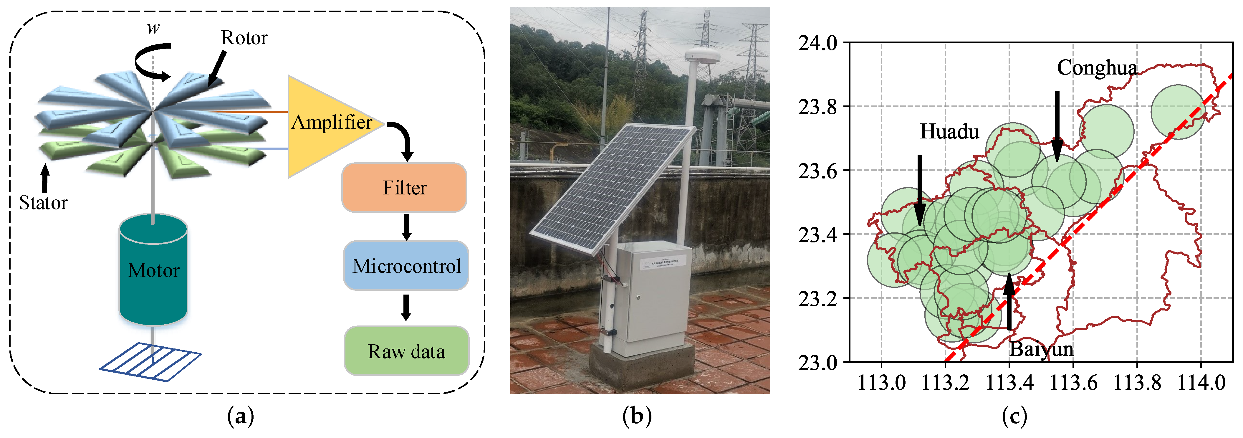
Figure 1. Atmospheric electric field meter and its distribution. (a) Schematic diagram of atmospheric electric field meter; (b) Physical view of atmospheric electric field meter; (c) Geographical distribution of electric field stations.
Remotesensing 14 04131 g001
Figure 2. Changes in electric field measurements at No. 1, No. 2, and No. 3 stations (19 August 2021, 12:30–15:30 CST).
Remotesensing 14 04131 g002
Figure 3. Lightning frequency statistics for the whole year of 2021.
Remotesensing 14 04131 g003
Figure 4. Schematic diagram for establishing thunderstorm weather samples and non-thunderstorm weather samples.
Remotesensing 14 04131 g004
Figure 5. Basic structure of the auto encoder.
Remotesensing 14 04131 g005
Figure 6. Visualization of electric field data.
Remotesensing 14 04131 g006
Figure 7. Architecture of ResNet50.
Remotesensing 14 04131 g007
Figure 8. Structure of the residual block.
Remotesensing 14 04131 g008
Figure 9. (a) Residual block structure of the standard ResNet50; (b) Improved residual block structure.
Remotesensing 14 04131 g009
Figure 10. Fine-tuning of the ResNet50 network.
Remotesensing 14 04131 g010
Figure 11. Several thunderstorm samples (the colored dots represent lightning that occurred during the corresponding time period and pink rectangular area represents the lightning’s gathering area).
Remotesensing 14 04131 g011
Figure 12. Fundamental structure of multilayer perceptron.
Remotesensing 14 04131 g012
Figure 13. Architecture of the lightning warning algorithm (the blue rounded rectangle is the time positioning module and the blue rounded rectangle is the space positioning module).
Remotesensing 14 04131 g013
Figure 14. MSE loss function training curve.
Remotesensing 14 04131 g014
Figure 15. Loss function and accuracy evolution of the training and validation sets during the training process.
Remotesensing 14 04131 g015
Figure 16. An example of atmospheric electric field data visualization.
Remotesensing 14 04131 g016
Figure 17. Test accuracies of four methods under noisy conditions.
Remotesensing 14 04131 g017
Figure 18. MAE and Loss training curves.
Remotesensing 14 04131 g018
Figure 19. Plot of lightning spatial localization results for space positioning module (the dots in the graph represent the difference between the predicted and observed latitude and longitude of the lightning).
Remotesensing 14 04131 g019
Figure 20. Performance of lightning localization. (a) Comparison of experimental results on the prediction of spatial localization by different lengths of electric field time series (the red and blue dashed lines represent the top values of the bar chart, respectively); (b) MAE and loss of space positioning module under noisy conditions.
Remotesensing 14 04131 g020
Figure 21. Three cases in the operation of lightning warning system (The green mark “x” represents the distribution of the atmospheric electric field meters, the blue numbers represent the actual center of flashes, the red numbers represent the predicted positions, and the numbers themselves represent the time elapsed compared to the start). (a) A thunderstorm that occurred on 2 May 2021 from 13:37 to 14:07; (b) A thunderstorm that occurred on 10 June 2021 from 15:29 to 15:59; (c) A thunderstorm that occurred on 17 August 2021 from 18:32 to 19:02.
Remotesensing 14 04131 g021
Table 1. Joint table of early warning results and observation results.
ObservationsPositiveNegative
PredictionPositiveTPFP
NegativeFNTN
Table 2. Comparison of experimental results on the prediction of lightning occurrence time by different lengths of electric field time series.
LengthEvaluation Metrics
PrecisionRecallF1Accuracy
300.85630.69450.76590.8068
350.90070.74540.81560.8447
400.87690.76070.81460.8416
450.88710.75750.81620.8440
500.90840.76400.82920.8561
550.89860.78680.83860.8616
600.92170.81470.86410.8817
Table 3. Results after data augmentation and comparison with the performance of other models (“-” denotes that data is missing).
MethodsEvaluation Metrics (%)
PrecisionRecall F 1 Acc
Without Aug92.281.586.488.2
After Aug90.889.890.390.4
Original Resnet5086.388.487.487.3
CNN85.987.886.886.8
LSTM84.386.285.385.2
Ref. [31]85.482.784.0-
Ref. [32]88.087.286.786.8
Table 4. Real lightning events and the predicted results given by the system per minute in Case 1 (to facilitate the display, the latitude and longitude data in the table are kept to two decimal places, and the original data to six decimal places were used to calculate “Distance” and draw Figure 21. (The “-” mark in the table represents missing data, and the same applies to the following tables).
Time (min)Number of FlashesCase 1
Geometric CenterPrediction PointDistance (km)
12(113.37, 23.51)(113.32, 23.41)12.65
2----
31(113.45, 23.69)(113.45, 23.55)16.04
4----
5--(113.31, 23.22)-
61(113.30, 23.18)--
7--(113.35, 23.25)-
8----
9----
101(113.12, 23.36)(113.21, 23.41)10.76
111(113, 23.42)(113.05, 23.38)7.34
121(113.17, 23.34)(113.11, 23.38)7.64
131(113.05, 23.41)(113.05, 23.31)10.59
141(113, 23.42)(113.12, 23.42)12.23
151(113.02, 23.39)--
16--(113.05, 23.35)-
172(113.07, 23.4)(113.12, 23.34)7.98
18----
192(113.03, 23.4)(113.11, 23.44)9.08
20----
211(113.03, 23.4)(113.12, 23.39)9.07
222(113.3, 23.33)--
234(113.09, 23.37)(113.06, 23.33)5.77
24----
253(113.06, 23.39)(113.08, 23.35)5
261(113.06, 23.38)(113.09, 23.32)7.88
273(113.02, 23.41)(113.11, 23.42)9.19
285(113.08, 23.34)(113.13, 23.36)4.95
294(113.03, 23.41)(113.06, 23.43)3.52
302(113.06, 23.39)(113.09, 23.46)8.14
3110(113.14, 23.29)(113.04, 23.35)11.78
Table 5. Real lightning events and the predicted results given by the system per minute in Case 2.
Time (min)Number of FlashesCase 2
Geometric CenterPrediction PointDistance (km)
12(113.52, 23.6)(113.38, 23.52)16.9
22(113.27, 23.43)(113.32, 23.43)5.14
32(113.27, 23.42)(113.26, 23.39)3.09
47(113.24, 23.45)(113.29, 23.45)5
5--(113.35, 23.41)-
6----
75(113.39, 23.36)(113.36, 23.34)3.78
84(113.23, 23.34)(113.33, 23.33)10.27
9----
104(113.26, 23.31)(113.30, 23.32)4.23
116(113.24, 23.35)--
126(113.3, 23.36)(113.32, 23.36)1.9
132(113.27, 23.35)(113.19, 23.38)9.15
149(113.25, 23.33)--
15----
168(113.22, 23.34)--
175(113.25, 23.35)(113.21, 23.36)3.96
183(113.26, 23.36)(113.31, 23.36)5.52
194(113.26, 23.36)(113.22, 23.32)5.75
202(113.25, 23.34)(113.3, 23.34)5.12
217(113.24, 23.34)(113.21, 23.4)7.38
22--(113.21, 23.5)-
236(113.21, 23.38)(113.18, 23.35)4.39
241(113.22, 23.35)(113.12, 23.38)10.58
251(113.26, 23.27)--
264(113.28, 23.38)(113.22, 23.46)10.6
279(113.2, 23.34)(113.26, 23.33)6.04
2817(113.22, 23.37)(113.27, 23.32)7.32
297(113.21, 23.33)(113.22, 23.29)4.33
309(113.22, 23.35)--
316(113.22, 23.37)(113.24, 23.42)5.83
Table 6. Real lightning events and the predicted results given by the system per minute in Case 3.
Time (min)Number of FlashesCase 3
Geometric CenterPrediction PointDistance (km)
11(113.23, 23.08)(113.38, 23.26)25.03
23(113.54, 23.48)(113.62, 23.59)14.53
38(113.56, 23.6)(113.61, 23.62)5.24
411(113.36, 23.25)(113.55, 23.52)35.69
54(113.57, 23.63)(113.61, 23.65)4.51
614(113.65, 23.68)(113.63, 23.62)6.94
714(113.67, 23.69)--
815(113.69, 23.76)(113.68, 23.64)13.5
98(113.63, 23.68)(113.58, 23.72)6.47
105(113.64, 23.68)--
1117(113.64, 23.65)(113.68, 23.72)8.72
122(113.74, 23.75)(113.72, 23.64)12.46
1316(113.66, 23.69)(113.66, 23.64)5.04
1430(113.61, 23.67)(113.65, 23.62)7.4
1518(113.64, 23.68)--
169(113.68, 23.71)--
1714(113.64, 23.68)(113.58, 23.62)8.83
187(113.62, 23.56)(113.62, 23.6)4.24
1945(113.62, 23.64)--
2015(113.64, 23.66)(113.52, 23.58)15.65
2110(113.62, 23.61)--
225(113.65, 23.68)(113.63, 23.62)6.94
2311(113.6, 23.61)(113.64, 23.6)4.66
2415(113.63, 23.64)(113.68, 23.58)8.3
259(113.59, 23.63)(113.52, 23.56)10.4
269(113.65, 23.65)(113.61, 23.56)10.89
2716(113.66, 23.68)(113.59, 23.68)6.66
2811(113.57, 23.6)(113.6, 23.59)3.57
2910(113.58, 23.62)--
3016(113.67, 23.56)(113.55, 23.66)15.99
316(113.57, 23.57)(113.61, 23.51)7.63
Publisher’s Note: MDPI stays neutral with regard to jurisdictional claims in published maps and institutional affiliations.