Evaluation of the Capability of ExoMars-TGO NOMAD Infrared Nadir Channel for Water Ice Clouds Detection on Mars

Abstract

As part of the payload of the 2016 ExoMars Trace Gas Orbiter (TGO) mission, the Nadir and Occultation for MArs Discovery (NOMAD) suite instrument has been observing the Martian atmosphere since March 2018. NOMAD is mainly dedicated to the study of trace atmospheric species taking advantage of a high-spectral resolution. We demonstrate that when NOMAD is observing in nadir mode, i.e., when the line-of-sight points to the centre of Mars, it can be also exploited to detect ice. In this study we present a method based on the investigation of nadir observations of the NOMAD infrared channel, acquired during Mars Years 34 and 35 (March 2018 to February 2021). We take advantage of the strong water ice absorption band at 2.7 µm by selecting the diffraction orders 167, 168, and 169. We derive the Frost and Clouds Index (FCI), which is a good proxy for ice mapping, and obtain latitudinal-seasonal maps for water ice clouds. FCI is sensitive to the Polar Hood clouds. Nevertheless, detections in the Aphelion Cloud Belt (ACB) are limited. This is consistent with previous observations showing different physical properties between the two main Martian atmospheric structures and making the ACB less detectable in the infrared. We hence derive the infrared nadir channel sensitivity limit for the detection of these clouds.

1. Introduction

Understanding the exchanges between the atmosphere and the surface remains pivotal in planetary climate research. On Mars, seasonal variations in the main atmospheric gaseous components are strongly affected by their condensation and sublimation within the polar caps [1]. In this framework, the formation of ice clouds plays a fundamental role in sculpting the Martian climate. By observing their spatial and seasonal distributions, we can improve our knowledge on atmospheric transport, as well as on water vapour and CO₂ cycles. Moreover, studying the formation and composition of ice clouds can help to better understand smaller scale phenomena such as convective regimes and thermal effects of radiative forcing [2].

Over the two past decades, water ice clouds have been deeply analysed in their composition, microphysical properties and vertical distribution [3,4,5,6,7,8,9,10], also identifying two main seasonal cloud structures emerging at a planetary scale: the Aphelion Cloud Belt (ACB) and Polar Hood (PH) clouds [11,12,13,14,15,16,17,18,19]. Important variations in the Martian topography can also promote the formation of water ice clouds. This is the case, for instance, of the highest volcanoes in the Tharsis region, where extremely elongated orographic clouds have been observed [20,21,22]. The interpretation of such observations can rely on theoretical circulation models needed for a comprehensive understanding of the Martian climate in its complexity [23,24,25,26,27,28,29,30]. These global climate models (GCMs) are in turn trained by continuously comparing their outputs with new observations. Further observations are hence always necessary.

In this work, we investigate the information content of the ExoMars-TGO NOMAD infrared channel nadir dataset. NOMAD is a suite of high spectral resolution instruments mainly dedicated to studying the Martian atmosphere trace gases and climatological processes [31,32,33,34,35]. Given the peculiar mode of operations of the instrument for nadir observations, it is difficult to discern clouds from suspended dust and surface ice deposits. For that reason, we define here a method aimed to identify H₂O ice clouds in NOMAD infrared nadir data, based on the characterization of the 2.7 μm ice absorption band. A brief description of the NOMAD instrument and of the nadir observations that we used in this study is presented in Section 2. Then, we describe the methodology of the study and derive the Frost and Clouds Index in Section 3. The analysis of NOMAD nadir data for MY34 and MY35 is performed in Section 4, where the results obtained over 1.5 MY of NOMAD acquisition are discussed and compared to previous studies and model predictions.

2. NOMAD Instrument

The Nadir and Occultation for MArs Discovery (NOMAD) instrument is a suite of three high resolution spectrometers that was selected as part of the payload of the 2016 ExoMars Trace Gas Orbiter (TGO) mission. Led by the Royal Belgian Institute for Space Aeronomy (BIRA-IASB), NOMAD has been observing the Martian atmosphere since March 2018 (L_S = 150° in MY34) through three channels operating in the ultraviolet-visible (UV-VIS), and infrared (IR) spectral ranges. A first spectrometer is devoted to solar occultation observations (SO channel), operating in the 2.3–4.3 μm IR spectral range. A second spectrometer, capable of performing nadir, limb, and solar occultation observations (LNO channel) covers the 2.3–3.8 μm IR spectral range. A third spectrometer (UVIS channel) can work in the three observation modes covering the 200–650 nm UV-VIS spectral range. A complete description of the instrument can be found in the following papers: Neefs et al. [36], Vandaele et al. [37,38], Thomas et al. [39], and Patel et al. [40].

In the present work, we select the LNO channel for the nadir observations covering the 2.3–3.8 μm IR spectral range with a spectral resolution of 0.3 cm⁻¹ [8]. This channel provides observations of the Martian surface and atmosphere with a typical integration time of around 200 ms. The ground track footprint is approximately 0.5 km × 17.5 km from the TGO orbit, 400 km above Mars. Therefore, NOMAD-LNO is able to map the majority of the surface of the planet every 30 sols [39]. The spectrometer does not observe the whole LNO spectral range simultaneously. Instead, acquisitions are performed nearly simultaneously in 22 cm⁻¹ wide spectral windows (called here orders from now on), representing specific diffraction orders of the diffraction grating. Considering the signal-to-noise ratio (SNR), a maximum number of 6 diffraction orders can be selected for each observation every 15 s, by suitably tuning the frequency of the entrance Acousto-Optical Tunable Filter (AOTF) [8] through an internal radio-frequency generator.

We use level 1A LNO data, which provides data converted into a reflectance factor, i.e., the LNO radiance divided by the measured Solar flux at Mars and by the cosine of the solar zenith angle. The LNO reflectance factor defined at wavelength λ can be written as

$$R_{\lambda }=\frac{1}{cos\left(SZA\right)} \frac{\pi L_{\lambda }}{{\Phi }_{Su{n}_{\lambda } }{d}_{Mars}^2}$$

(1)

where L_λ is the LNO measured spectral radiance (W m⁻² sr⁻¹ μm⁻¹), Φ_Sunλ is the Solar flux at 1 astronomical unit (AU), d_Mars is the Sun–Mars distance in AU, and SZA is the solar zenith angle. More details about the LNO calibration we adopt are presented in Thomas et al. [41]. A slightly different calibration approach, in agreement with the former, within 3%, is given by Cruz Mermy et al. [42].

It is important to note that the general shape of the NOMAD raw spectra is strongly affected by the AOTF transmission and by the spectral response of the grating, i.e., the Blaze function [39]. While the Blaze function is defined by a Gaussian curve, the AOTF transmission presents a strong peak with several side-lobes. A combination of a sinc function with a Gaussian is used to represent the AOTF curve [8]. Nevertheless, these secondary peaks allow photons from a larger spectral range to fall on the grating. As a result, an unexpected signal is summed with the expected spectral information. This becomes significant on the edges of each order. After the spectral and radiometric calibrations [8,41,42], the AOTF and Blaze modulations also propagate to the reflectance factor conversion in the form of low-frequency oscillations in the spectral continuum. For this reason, we only work with reflectance factors at the central value of each spectral order in order to mitigate these oscillations.

Regarding the SNR of the data, Thomas et al. [39] made an analysis taking into account different sources of uncertainty. The main source of noise is represented by the instrument thermal background, which limits the integration times in order to avoid the saturation of the detector. The 15 s period of observations is divided by the number of orders (maximum of 6). Therefore, measuring fewer orders achieves a better SNR. In the same sequence of observations, two or three orders are typically measured, given an average SNR value of 10. For the best scenario, strongly affected by SZA, the measured SNR is expected to be around 15–20 [41].

3. Methodology

3.1. Data Selection

The first step of this work is to identify the water ice spectral features covered by NOMAD diffraction orders. A brief description of the spectral content and main scientific focus of each available LNO diffraction order is presented in Oliva et al. [43], who discussed the capability of the NOMAD infrared nadir channel to detect surface ice by using a spectral ratio with orders 190 (2322.9–2341.5 nm) and 169 (2611.8–2632.7 nm). These two orders allowed estimation of the relative depth of the 2.7 μm absorption band, which is the strongest CO₂ and H₂O ice absorption band in the LNO spectral range. However, this approach is less effective for the detection of transient phenomena such as ice clouds. It hence requires a more stringent temporal and spatial coincidence between the two orders. Nevertheless, as detailed in Section 2, NOMAD is not capable of observing its entire spectral range simultaneously due to its mode of operation and high resolution. Therefore, NOMAD alternates observations according to diffraction orders. As a result, the observation period of order 190 does not fully coincide with the other. We are therefore very limited in the temporal coverage. For this reason, we investigate an alternative approach focused on orders 169 (2611.8–2632.7 nm), 168 (2627.2–2648.2 nm) and 167 (2642.8–2663.9 nm), all falling on the short-wavelength shoulder of the strong 2.7 μm ice absorption band (see Figure 1).

Figure 1 presents simulated CO₂ ice, H₂O ice, and dust reflectance spectra using the Multiple scattering Inverse radiative TRansfer Atmospheric (MITRA) tool [44,45,46,47]. MITRA code is based on the multi-solver LibRadtran radiative transfer package [48] and can be operated both as a forward model and as an inverse retrieval algorithm to study planetary atmospheres [44,45,46,47]. In this study, we take advantage of the forward model in order to reproduce spectra in the LNO spectral range. Nevertheless, we do not attempt to derive aerosol microphysical information. Indeed, as we work in nadir mode, the signal is highly convoluted with the surface properties and therefore, abundance and grain size retrievals are characterised by non-negligible uncertainties when using only a few orders. Regarding the ice reflectance spectra, surface CO₂ ice and H₂O ice are simulated with effective radii of 100 µm (r_eff = 100 µm) (dark/light blue solid lines), while r_eff = 7 µm and 10 µm are respectively used for CO₂ ice and H₂O ice clouds (dark/light blue dashed lines). Conversely, the red solid line represents the dust spectrum with r_eff = 1 µm [43]. As highlighted by the vertical dashed green line, order 190 is located on the ice cloud continuum. The challenge of this work is to define a technique that exploits only orders 167, 168, 169 and that allows detection of H₂O ice clouds and frost separated from dust (see Section 3.2 and Section 4.2).

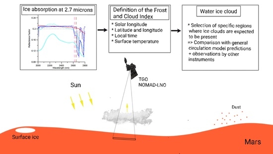
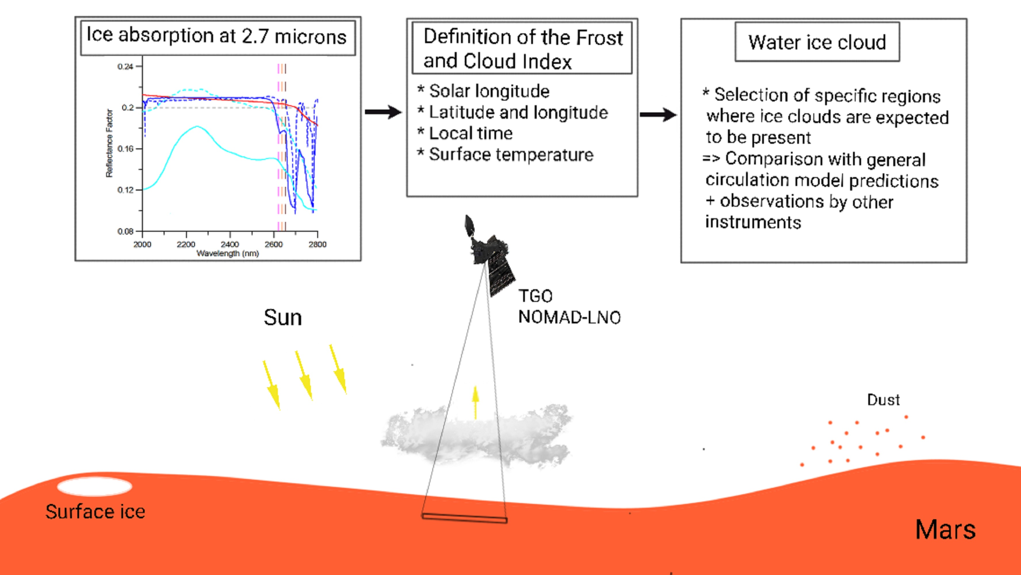
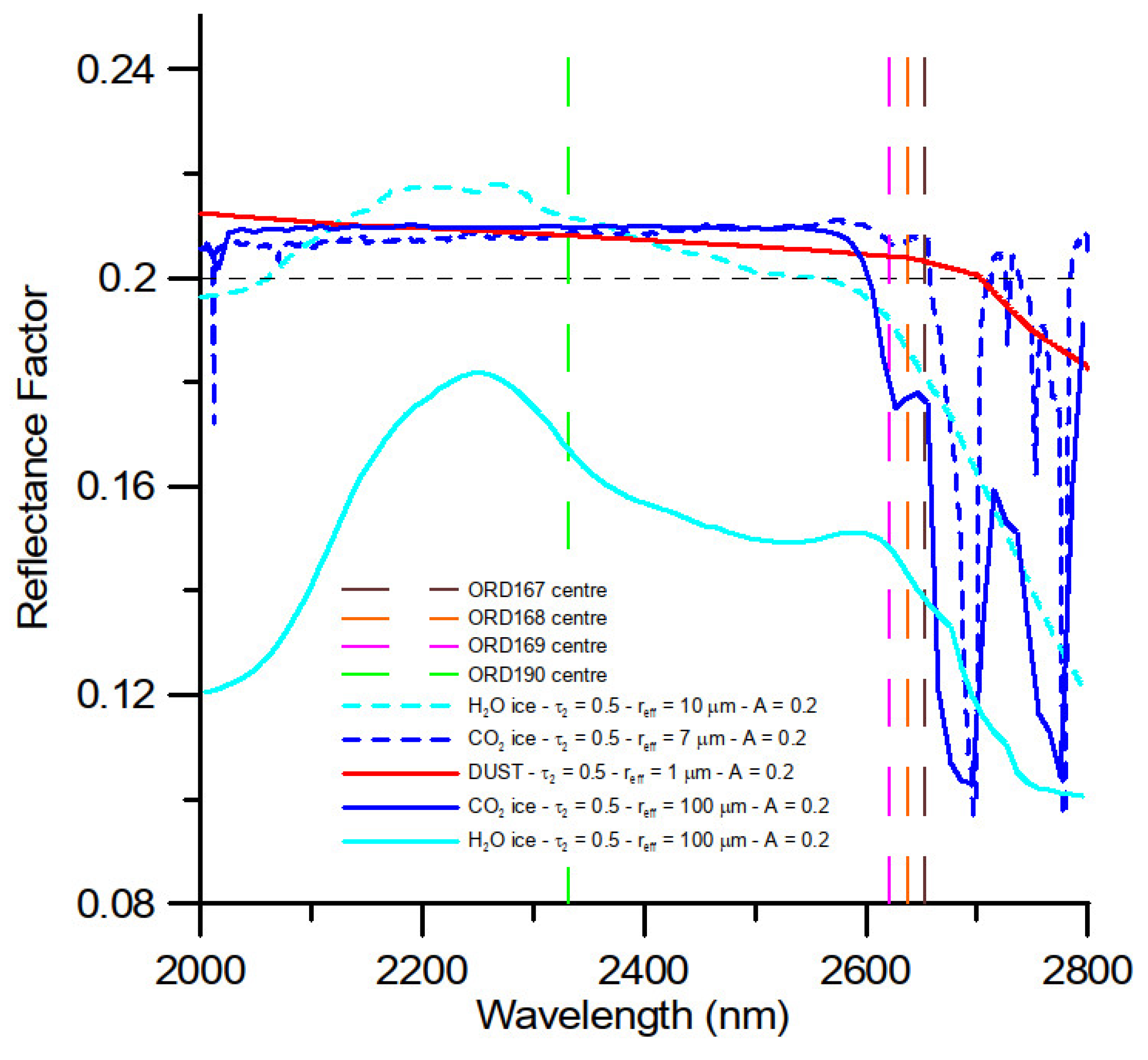
3.2. Frost and Clouds Index through the 2.7 µm Absorption Band

In the LNO spectral range, the surface reflectance is the main source of signal variability. Therefore, any effort to detect ice cloud’s spectral signatures has to account for the surface contribution. Previous studies using MGS-TES [49], MEX-OMEGA [50], and CRISM [51] nadir observations have demonstrated albedo spatial variations over the whole Martian surface [49,52,53]. These albedo variations, coming from different surface mineralogy absorptions, also represent the main source of variability in LNO reflectance factors. By comparing LNO reflectance to a Martian albedo map it is possible to remove surface albedo contributions and to spotlight anomalous detections resulting from, for example, an ice cloud’s spectral signature. To this extent, OMEGA data provide reflectance spectra in the NIR allowing the construction of albedo maps in the 0.97–2.7 µm spectral range [53]. Nevertheless, as cautioned by Riu et al. [54], OMEGA albedo maps can be partially biased in low-albedo equatorial terrains, where plagioclase minerals predominate [54,55,56]. Indeed, in the NIR, this mineral phase presents a lack of spectral absorption features that may be altered by the presence of dust and could constitute a caveat for the construction of OMEGA albedo maps. On the contrary, TES is able to detect plagioclase features in the TIR range [55], and therefore, takes into account the low-albedo equatorial terrains effect on the NOMAD spectra. Moreover, TES data are also filtered to partially minimise the effect of atmospheric dust and clouds. For these reasons, we will rely on the TES bolometric albedo (0.3 to 2.9 μm), instead of the NIR OMEGA albedo (0.97–2.7 µm), as a reference for evaluating anomalies in the LNO reflectance factors.

For each LNO observation, i, characterised by different longitudes and latitudes, we define for simplicity the LNO_Norm ratio as

$${\left(LN{O}_{Norm}\right)}_i=\frac{R_i}{TE{S}_i}$$

(2)

where R is the reflectance factor value taken at the centre of the selected order (i.e., at λ = 2622.3 nm, 2637.8 nm, and 2653.6 nm for orders 169, 168 and, 167 respectively), and TES is the bolometric Martian albedo value averaged in each considered LNO footprint. Such a ratio will be sensitive to anomalies pertaining to both ice and dust, and for this reason, we investigate how it behaves with the two components by performing simulations with the MITRA tool.

Figure 2 illustrates LNO_Norm simulations of dust and H₂O ice, adopting average effective radii and optical depths, and considering order 169 as an example (dashed lines). The ice absorption makes the resulting curve depart significantly with respect to the dust curve. Conversely, the same behaviour is not observed in order 190, also shown in Figure 2 as reference, where the two curves are quite similar (solid lines). It is important to stress that changing the aerosol’s microphysics in the simulations has an impact on the LNO_Norm value, in principle making dust mimic ice anomalies especially on low-albedo terrains and hence, possibly yielding false positive detections.

Given that LNO data moderate SNR, the LNO_Norm parameter is affected by non-negligible fluctuations. In order to mitigate this effect, we combine LNO_Norm of the three orders defining a Frost and Clouds Index as

$$\mathrm{FCI}=\frac{1}{LNONorm 167 \ast LNONorm 168 \ast LNONorm 169}$$

(3)

where LNO_Norm 167, LNO_Norm 168, and LNO_Norm 169 are respectively the LNO_Norm values defined in Section 3.2 for orders 167, 168, and 169.

Similarly to Figure 2, simulations have been performed for FCI in the presence of suspended dust and water ice particles (see Figure 3). Given the way FCI is defined, as expected, its simulated values are larger for water ice (blue line). While the LNO_Norm ratio allows to spot anomalous detections in presence of water ice clouds, FCI allows to emphasise simultaneous detections happening in the three orders and helps to potentially derive a threshold value for ice detection as will be shown in Section 4.1. Nevertheless, it is important to mention that, despite the TES map being filtered to minimise the effect of atmospheric dust and clouds, it still contains surface ice [49], increasing the uncertainty in transitional ice/no-ice regions. As in the case of the Ice Index [43], the discussion coming from the FCI is semi-qualitative and the value that we derive later should not be considered as an actual threshold for ice detection, but rather an indication for abundant frost or dense water ice clouds.

4. Data Analysis and Results

For this study, we analyse 1.5 Martian Years of NOMAD LNO nadir infrared observations thanks to the three orders mentioned in Section 3.1.

Table 1. Number of LNO orbits through the 3 orders close to the 2.7 μm ice absorption band (i.e., 169, 168, and 167) in MY34 (starting at L_S = 150° which is the beginning of the NOMAD science phase) and MY35.

	MY34: LS = [150–360°]	MY35: LS = [0–360°]	Total
Order 167	682	371	1053
Order 168	504	1144	1648
Order 169	694	403	1097
TOTAL	1880	1918	3798

presents the number of orbits acquired for each order. Even if order 168 has been deeply used in MY35, we globally note a fair distribution in the total number of observations between MY34 and 35.

In order to focus the analysis on seasonal ice coverage, we construct a latitudinal-seasonal map of FCI (see Figure 4). Initially, all the LNO data are organised by latitude (from 90°N to 90°S) and time (MY34 and 35), expressed in terms of L_S, with a 2° × 2° binning. Each bin of latitude and L_S contains data averaged at all available longitudes. By computing the FCI map, we keep track of the observations falling into common bins for all the three orders. Then, we remove the worst-case scenarios with the lowest SNRs, i.e., below SNR~10. We hence select the LNO observations with a solar zenith angle lower than 60°, as larger illumination angles seriously affect the signal intensity measured by NOMAD. In order to keep a significant colour dynamic, in Figure 4 we saturate the colour bar for FCI values larger than 3. Important saturations can be observed at the highest latitudes in both hemispheres, i.e., when L_S = 180–270° in MY34–35 in the Southern hemisphere and when L_S = 0–45° in MY35 in the Northern hemisphere. These observations represent the sublimation phase of the polar cap [1,43,57,58,59,60,61]. Indeed, surface ice presents a strong absorption at 2.7 µm (see Figure 1) and directly impacts the FCI values. The polar regions are deeply discussed in Oliva et al. [43], which investigates the LNO information content in order to obtain latitudinal-seasonal maps for CO₂ ice in both polar regions. Being outside the scope of this paper, the polar caps observations are not discussed in detail here.

However, we observe bins with a high FCI value also in non-polar regions. In the Northern hemisphere, most of them can be found above latitude 40°N. Some high FCI values are also present around the equator for L_S = 45–180° in MY35. In the South, from latitude 20°S to 40°S, FCI returns some saturated pixels for L_S = 150–180° in MY34 and around L_S = 90° in MY35. The investigation of these non-polar high FCI pixels is discussed in the following section. First, we discuss the sensitivity of FCI to detect frost (see Section 4.1). Then, we attempt to derive a detection limit for water ice clouds (see Section 4.2).

On the other hand, as already mentioned in Section 3.2, different surface mineralogies are responsible for the global variations of surface albedo [62,63,64]. This affects the measured reflectance, especially over regions of low surface albedo [18,52]. It is worth noting that the high FCI values around latitude 60°N are over low surface albedo regions. This dark latitudinal band covers Acidalia and Utopia Planitia [65]. Szantai et al. [18] studied the diurnal cloud life cycle over these large regions using OMEGA data. Similar to the NOMAD data analysis in this work, they defined a spectral ratio (Reversed Ice Cloud Index (ICIR) based on Madeleine et al. [16]) at the 3.1 µm water ice absorption band and used it as a proxy of the water ice column. The results are not always in agreement with the model predictions. They found the highest ICIR uncertainty (>20%) over Acidalia and Utopia Planitia, regions with low surface albedo. For that reason, we also investigate the possibility of having surface effect residues in the results (see Section 4.3).

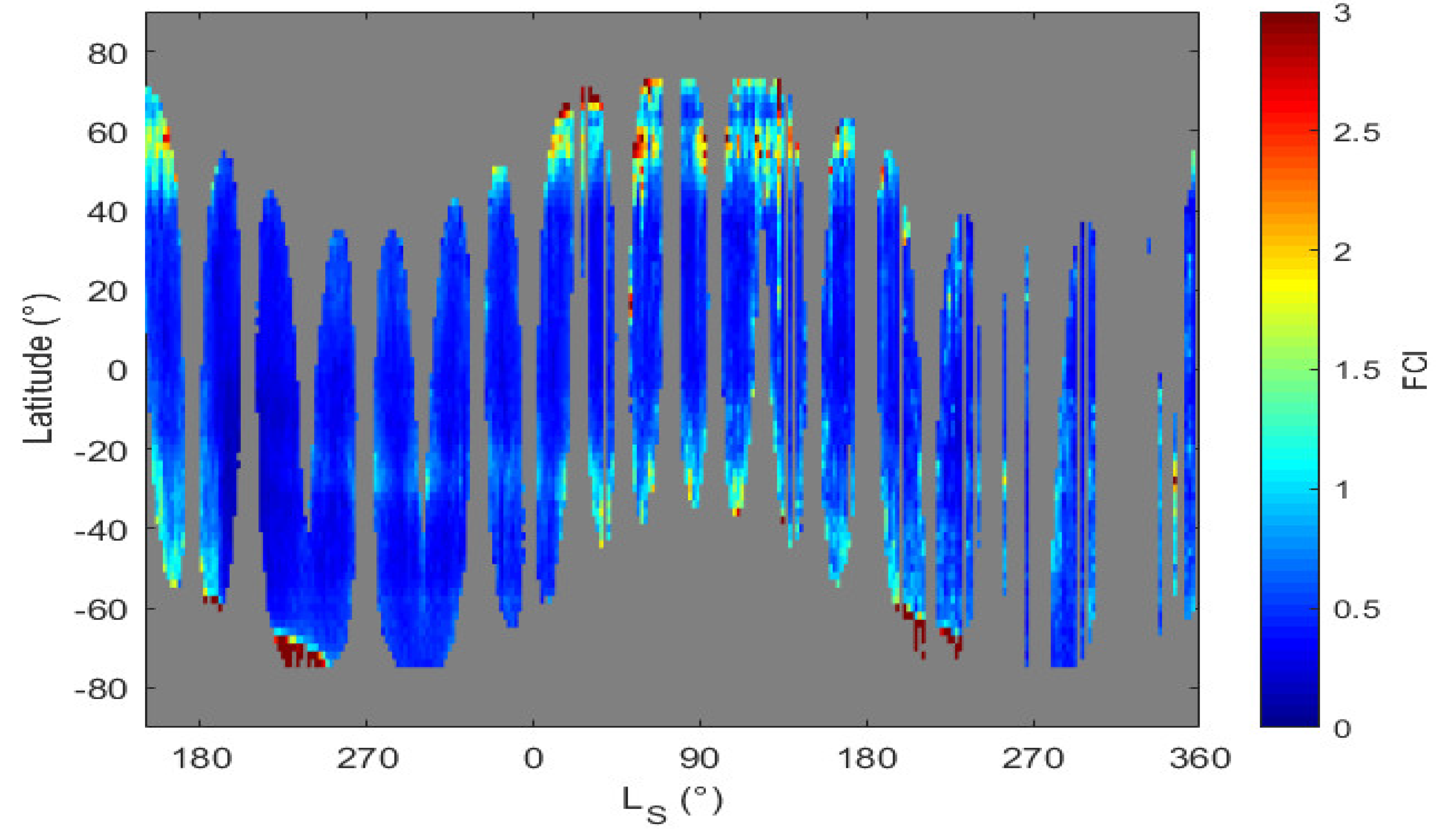
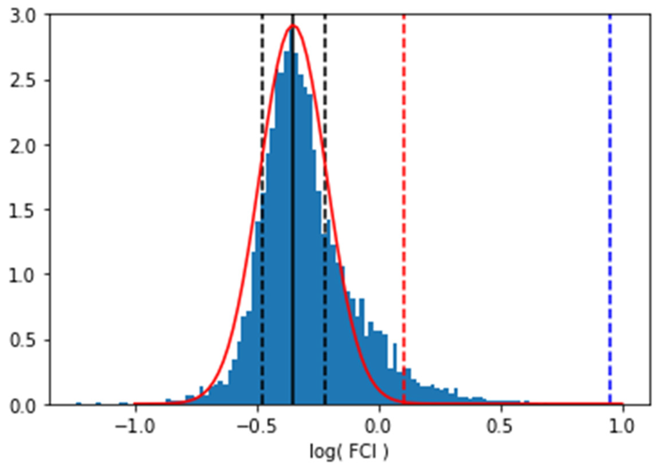
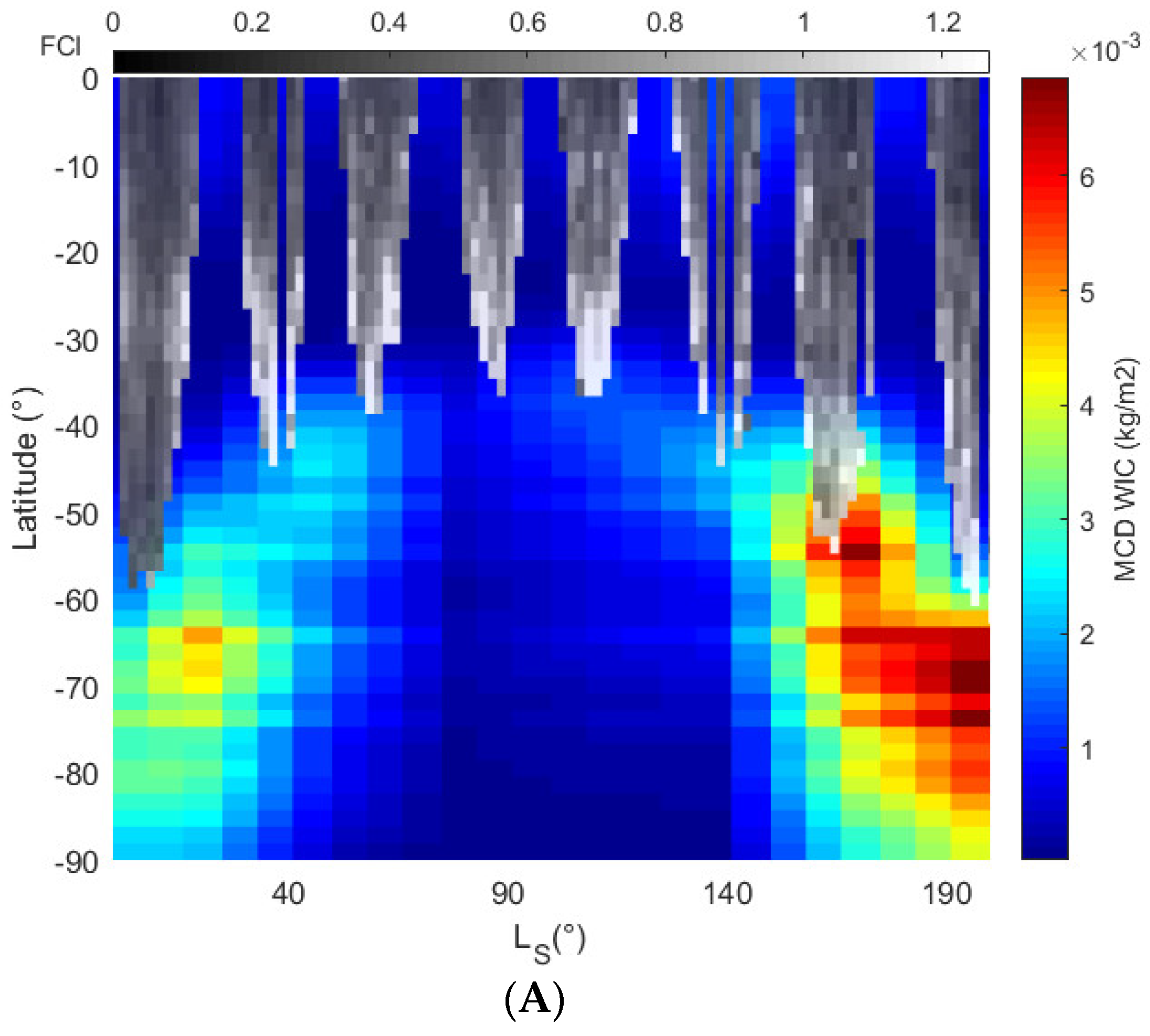
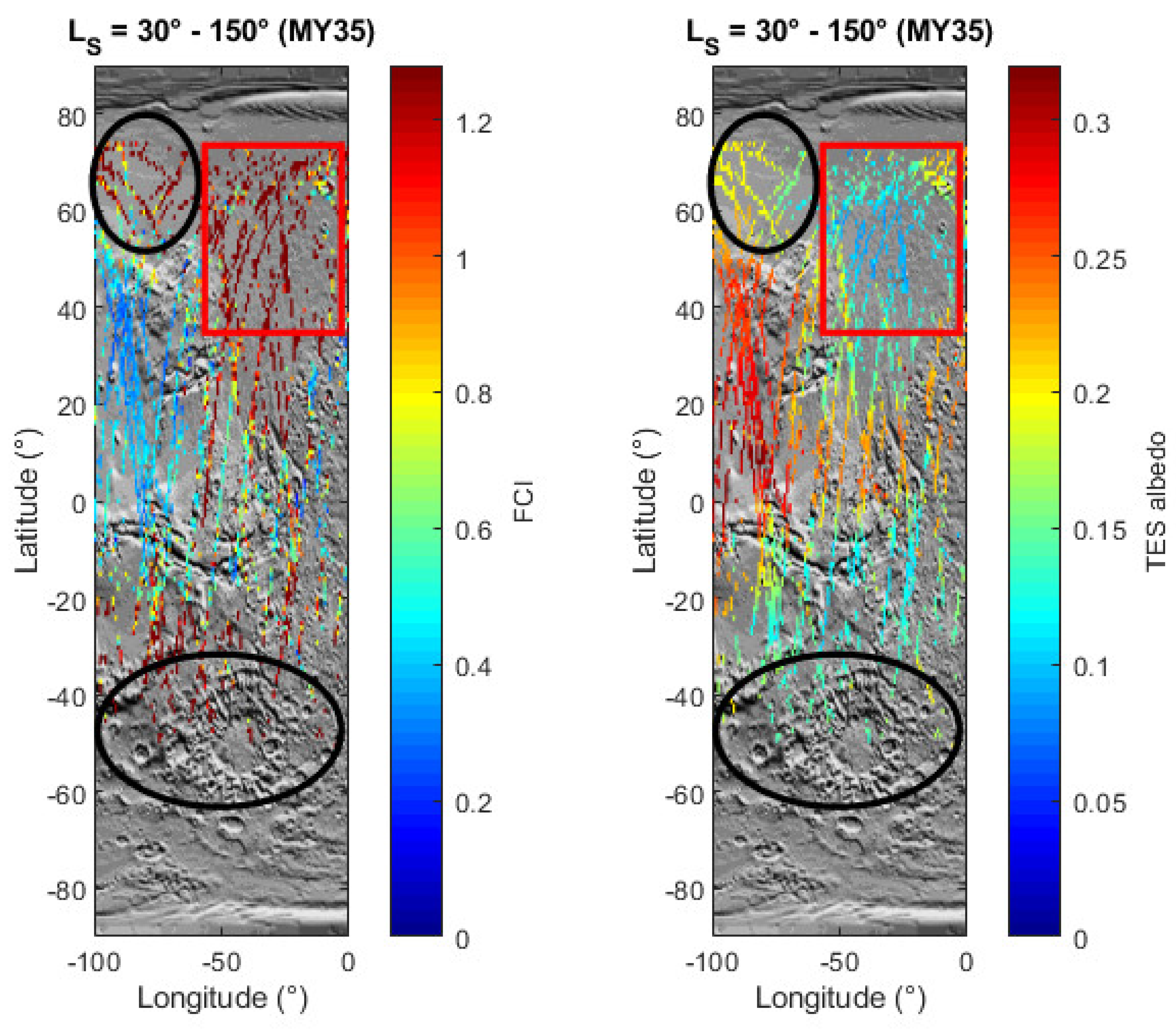
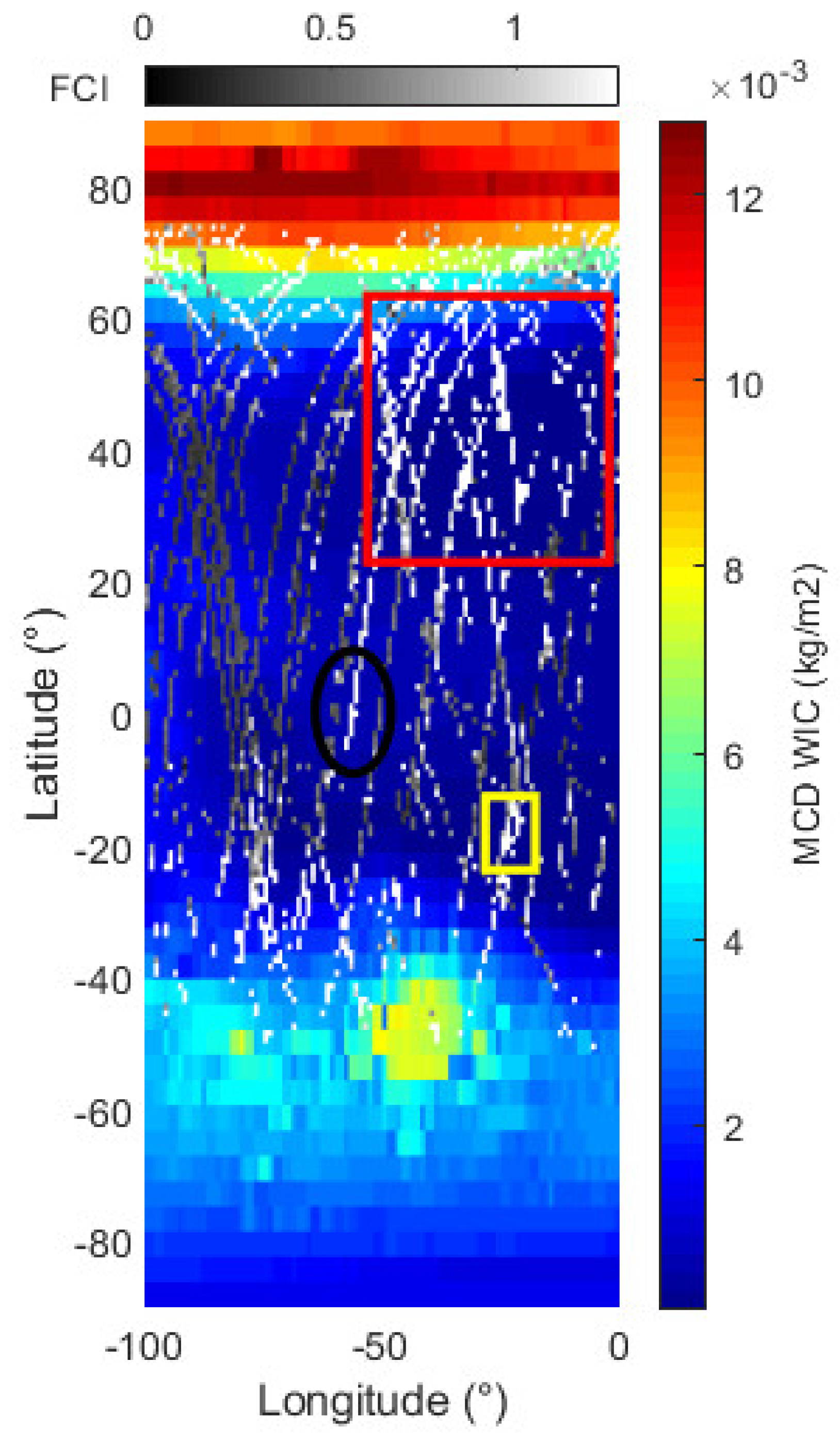
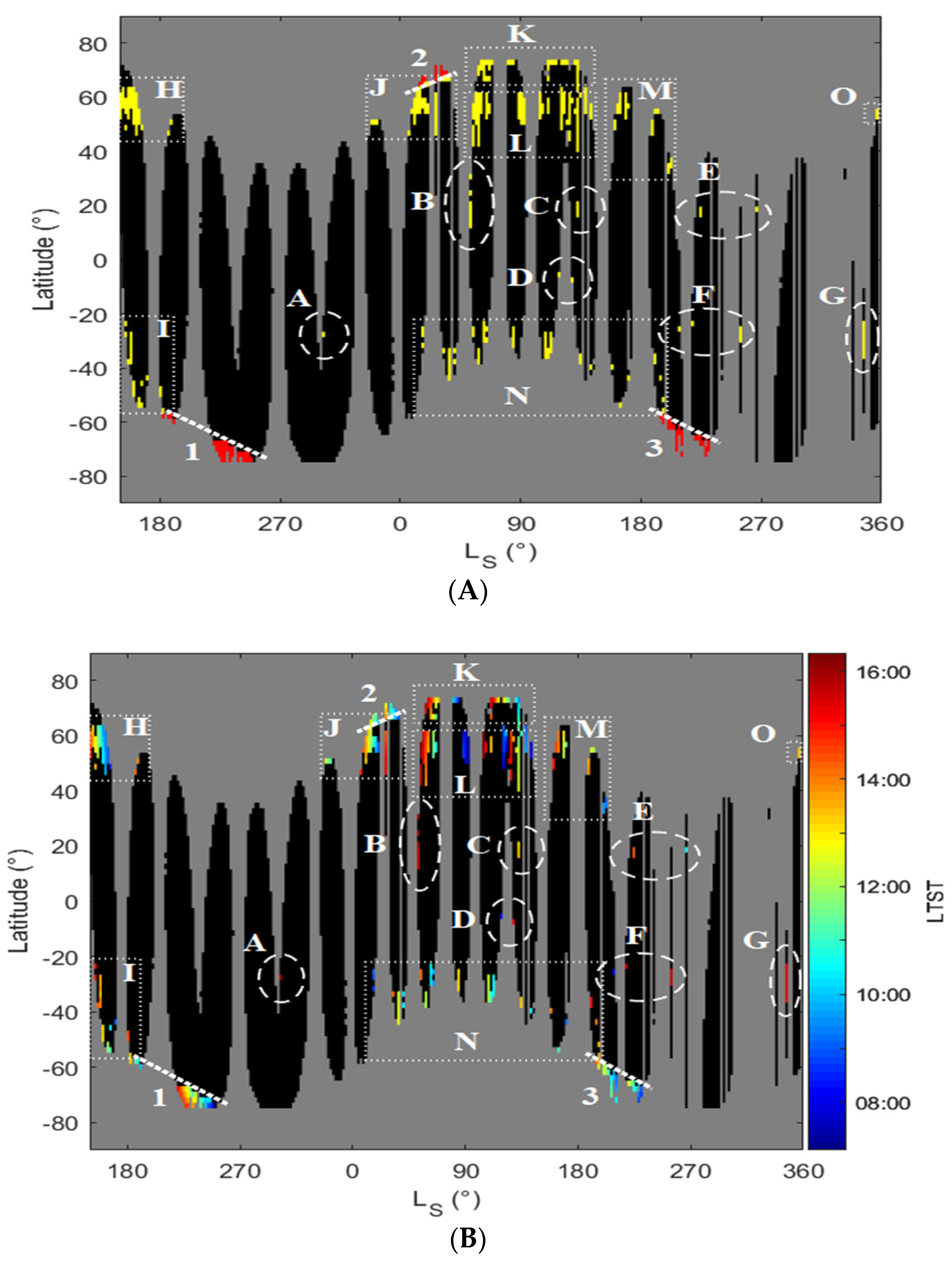
4.1. Frost Detection

We discuss here the possibility to derive a threshold value for the detection of frost. In order to define a quantitatively and statistically robust threshold value, we compute the histogram of FCI values distribution in logarithmic X-scale. As shown in Figure 5, the bulk of the histogram follows a Gaussian distribution peaked at −0.35 (µ = −0.35) with a standard deviation of 0.13 (σ = 0.13). Nevertheless, the distribution is not totally symmetrical around its mean value. We can observe a wing on the right-hand side of the distribution, corresponding to the high FCI pixels in Figure 4. Similarly to what has been done by Oliva et al. [43], we are able to tune the threshold value so that the edge of polar caps is detectable. This happens for FCI values exceeding the average value of the distribution by 3.5σ. This threshold is indicated by the vertical dashed red line in Figure 5. As a comparison, we also estimate an average FCI value for polar deposits, represented by the vertical dashed blue line (Figure 5). Sensitive to surface ice deposits, the FCI value over the polar cap exceeds the average value of the distribution by 10σ.

We apply it on the FCI map of Figure 4 and present the results in Figure 6A. As expected, detections in the polar regions (see regions 1, 2, and 3 in red) are in good agreement with the expected boundaries of the polar caps, but high values of FCI are also found at mid-latitudes. We now focus on these detections found at latitudes within the range of +/−30° (see regions from A to G in Figure 6A). A possible explanation for these detections is the presence of ice surface deposits. In order to verify this hypothesis, we need to take into account two parameters: the surface temperature (T) and the Local True Solar Time (LTST). Indeed, even at mid-latitudes, temperatures may drop below the frost point, i.e., T~148 K for CO₂ [66] and T~193 K for H₂O [67] at 610 Pa (average Martian pressure at 0 elevation). This can be achieved in the early morning just after the sunrise. Piqueux et al. [66] observed surface temperatures consistent with CO₂ frost at all latitudes and predicted a survival time of less than 1 h after sunrise. On the other hand, the Martian topography may play an important role, especially within ancient volcanoes, cracks, and craters. This complex geometry of terrain allows the existence of shadowed areas on a local surface, which can maintain low temperatures even during the day. Taking into account the LTST (see Figure 6B), we use the Mars Climate Database v5.3 (MCD) [25,68] in order to estimate the surface temperature for the mid-latitude detections in the end of MY34 (region A) and MY35 (from region B to G). For all these detections, the MCD predicted surface temperatures are listed in

Table 2. Solar longitudes (L_S), latitudes, local times (LTST), and MCD predicted surface temperatures (T) of the regions of interest (A to F) identified in Figure 6. Numbers in the regions D, E, and F represent bins from left to right in each region.

Region of Interest	LS (°)	Latitude (°)	LTST	T (K)
A	301 (MY34)	−27	16:12	282
B	51	11 to 29	16:00	254
C	133	16 to 21	13:18	236
D1	117	−5	08:25	220
D2	129	−7	15:40	260
E1	225	17	15:55	251
E2	267	19	10:43	253
F1	205	−25	8:20	240
F2	218	−23	15:56	279
F3	255	−24 to −30	15:57	286
G	347	−23 to −36	15:38	265

. It can be seen that MCD predicts surface temperatures that are always higher than the H₂O frost point (T > 193 K). We can hence exclude the presence of both CO₂ and H₂O frost even for 8:20 and 8:25 LTST, where residual night frost can survive (see Table 2 for D1 and F1). Moreover, the MCD predictions for the regions A, E, F and, G seem consistent with Carrozzo et al. [67] who observed H₂O frost only before L_S = 150°. In contrast, as mentioned above, frost can survive in shadowed regions along scarps and craters. However, this possibility is not easy to verify due to the large NOMAD nadir channel footprint (see Section 2).

Given the above discussion, we see that the interpretation of mid-latitude detections (regions A to G in Figure 6A) as surface frost can be discarded. In contrast, the detections in the regions B, C and, D fall in the Aphelion season, i.e., L_S~60–160°. During this season, the Aphelion Cloud Belt occurs every year at low latitudes. Therefore, these regions could be suitable for ACB detections. Moreover, in Figure 6A, we can also see many detections present at high latitudes (above 40°N and below 30°S in MY34-35) which relate to another important atmospheric structure, the Polar Hood. We hence decide to verify the cloud hypothesis in the next section by selecting specific regions where clouds are expected to be present by general circulation models or have been observed by other instruments.

4.2. Water Ice Cloud Detection

As already mentioned in the previous section, Figure 6A presents high FCI values even outside the red regions 1, 2 and, 3. In the Northern hemisphere, they are found above latitude 40°N. Moreover, we observe high values in the Southern hemisphere, mainly before L_S 180° (MY34) and around L_S 90° (MY35), in addition to the scattered detections at mid-latitudes (see Section 4.1). In this section, we verify the possibility to spot potential clouds using the FCI. To this extent, we highlight new regions of interest in which the detections are spotted (see the regions H to O in Figure 6). As we can observe, for the regions H to O in Figure 6b, the LTST mainly concentrates in a range of about 2 h around noon. Nevertheless, early detections exist in region L (see at L_S 90° and 164° and latitudes around 50°N), with a 7:13 LTST and 8:45 LTST respectively. MCD simulations always predict surface temperatures higher than 197K and are, therefore, inconsistent with the presence of frost. For this reason, we suggest that the detections are related to atmospheric ice (see Section 3). However, it is important to keep in mind that this region may lead to surface effect residues present in the results (see Section 4 and Section 4.3 for more details).

Two main cloud structures can be observed on Mars: the Polar Hoods (PH) and the Aphelion Cloud Belt (ACB) (see Section 1) [4,9,17]. The PH occurs above the high latitudes (~40°N and ~40°S) of the winter hemispheres. The Northern Polar Hood (NPH) is usually observed about three-quarters of the Martian Year, starting at L_S 150°, and covers all longitudes. Moreover, the NPH is always extended to the pole [15]. Instead, the Southern Polar Hood (SPH) is an annular ring that is not extended to the pole due to less available water vapour in the South than in the North [12]. The SPH is only present during two phases: between L_S = 10–70° (phase 1) and between L_S = 100–200° (phase 2) [14]. During phase 1, the structure is extended over a large range of latitudes, namely from 30°S to 75°S. As shown in region N, FCI detections are present from latitude ~25°S to 50°S. Given the period of observations (L_S = 0–200°), the FCI results appear to be compatible with clouds in the SPH. Figure 7 presents a direct comparison with the MCD simulations. However, the limited coverage for the Southern hemisphere does not allow us to observe the whole cloud structure. Nevertheless, we are able to observe the evolution of the SPH at equatorward latitudes. Detections between L_S = 15–83° appear compatible with phase 1. On the other hand, phase 2 seems to cover L_S 107° to 195°, following the recession of the polar cap. This phase is partially observed in region I (L_S = 153–187°) due to the lack of observations in MY34. Moreover, it is worth noting that the specifics of the TGO orbit influence the spatial and temporal coverages of the NOMAD observations. Indeed, as shown in Figure 6B, the LTST changes over the latitudes and L_S. Nevertheless, important diurnal variations of water ice clouds occur in the Martian atmosphere. Such effects can hence affect the results, underestimating the presence of clouds compared to the MCD predictions [19,69]. For example, at L_S 20°, observations are acquired in the morning for the Southern Hemisphere. At that time, MCD predicts a low water ice column at the probed latitudes (see Figure 7A). On the other hand, at Ls~100°, MCD simulations seem to be more in agreement with the FCI results by selecting a LTST in the early afternoon (see Figure 7B).

In the Northern hemisphere, we observe detections at the highest probed latitudes (see the regions J, K, M and, O) and around latitudes 50°N and 60°N (see the regions H and L). Detections in the regions H and M are compatible with the start of the NPH. Nevertheless, the limited coverage considerably reduces the number of observations during the northern autumn and winter in MY34 and 35. On the other hand, the regions J and O appear in agreement with the end of the NPH. During spring (before L_S 40° in region J), the FCI indicates the presence of clouds up to latitude 50°N, suggesting an extended NPH. During the rest of spring and summer (L_S~50–150° in region K), detections are not consistent with previous studies [9,10,15,17]. It is important to mention that the NOMAD instrument provides simultaneous observations of these clouds in the UV through the UVIS channel (see Section 2), that is sensitive to clouds and confirms their presence at latitude ~74°N (personal discussion with Y. Willame, ice clouds retrieval based on Willame et al. [17]). Moreover, these results are also supported by the MCD predictions. Nevertheless, FCI detections in region L are uncommon, especially between L_S~50° and 150°. At L_S~50° and 150°, they cover latitudes up to 35°N. A possible explanation is that they are related to the northern part of ACB, which seems to connect with the NPH. Although these detections are not predicted by MCD, they probably represent the so called ‘cloud bridge’ [70] detected during previous Martian Years [6,14,17,18,71,72]. Given the disagreement between the model predictions and FCI detections, we decide to discuss the results for the region L in the next section.

Regarding the ACB, it is not visible in our results in Figure 6. The structure is known to appear at low latitudes (10°S to 30°N), with enhancements over volcanoes in the Tharsis region [13]. Different types of clouds compose the cloud belt, ranging from formless morning thin haze to large-scale thick clouds. In terms of microphysical properties, two main groups have been observed for the thick clouds. The difference in particle size defines the core and the periphery of ACB. The first group corresponds to regions strongly controlled by local dynamics and topography. These clouds are observed over the Tharsis region with a 5 µm grain size. On the other hand, regional wind circulation forms the second group composed of large-scale clouds and is characterised by particle sizes of 2–3.5 µm [5,16]. In our results (Figure 6), only a couple of detections are present at equatorial regions during this season (see regions B, C and, D) and could be explained on the basis of the differences in morphology and microphysical properties described above. One of the reasons could be that the large LNOs footprint (Section 2) makes it difficult to detect optically thin hazes and clouds. On the other hand, large-scale cumulus clouds, from 5 to 10 km in size, could be detectable in the NOMAD nadir footprint. Nevertheless, they are relatively thin at the beginning of the northern spring and only become thicker late in the ACB season. The thickest of these clouds have been observed during the early northern summer, forming at the beginning of the afternoon [16,20] consistently to the regions C and D. Moreover, the clouds’ ice abundance could play an important role in their detection. Olsen et al. [10] derived the water ice column (WIC) for MY26-32 using the nadir IR observations of OMEGA. They estimated two ranges of values, about 1.2–1.6 pr. μm over the ACB and 1.5–2.5 pr. μm over the PH. This distinction between the two cloud structures can explain the global results presented in Figure 6. While we register several detections over the PH, only a few isolated clouds are detected over the ACB. This behaviour suggests that the LNO nadir dataset is only sensitive to clouds with ice columns larger than 1.5 pr. μm.

As mentioned in Section 4.1, detections are also present at mid-latitudes during the perihelion season (L_S = 180–360°, see regions A, E, F and, G in Figure 6). These results are difficult to confirm with the MCD predictions, although the simulations agree with the presence of clouds in region E for a 10:30-11 LTST. Moreover, the results for the regions A, E and, F are not consistent with the OMEGA data analysis [10]. During the perihelion season, the solar flux increases and relatively warms the Martian atmosphere promoting dust activity. This hence limits water ice cloud column opacities [12]. Nevertheless, previous works have demonstrated the presence of water ice clouds during this period. They mainly occur in the mesosphere (at altitudes above 50 km) [4,8,73]. The results in the regions A, F, and G appear to be in agreement with the previous studies focused on MRO-CRISM [51] and NOMAD-SO (SO channel, see Section 2) data analysis [4,8]. They spotted water ice clouds around L_S 200°, 270°, 300°, and L_S 345°, which were also observed by SPICAM [17] for the regions A and G. Moreover, especially for the regions A and F, the detections correspond to the period of the perihelion cloud trails (PCT). This class of mesospheric clouds are formed between L_S 210° and 310° in the late morning to the mid-afternoon. Horizontally extended (200 to 1000 km), they are observed over specific regions between latitudes 5°S and 40°S, i.e., in the Arsia Mons, Syria, and Solis regions and along the Thaumasia Planitia, Valles Marineris margins, and the north east of Hellas Basin [74,75].

Given the above discussion, it is important to remind that the kind of threshold value that we use indicates abundant frost or dense water ice clouds instead of an absolute value for ice detection (see Section 3.2 and Section 4.1). Therefore, the FCI appears to be sensitive only to ice that is characterised by a particular microphysics. Nevertheless, some FCI detections (especially region L in Figure 6) are still difficult to justify with previous studies or the MCD predictions. For that reason, we discuss these results in the next section.

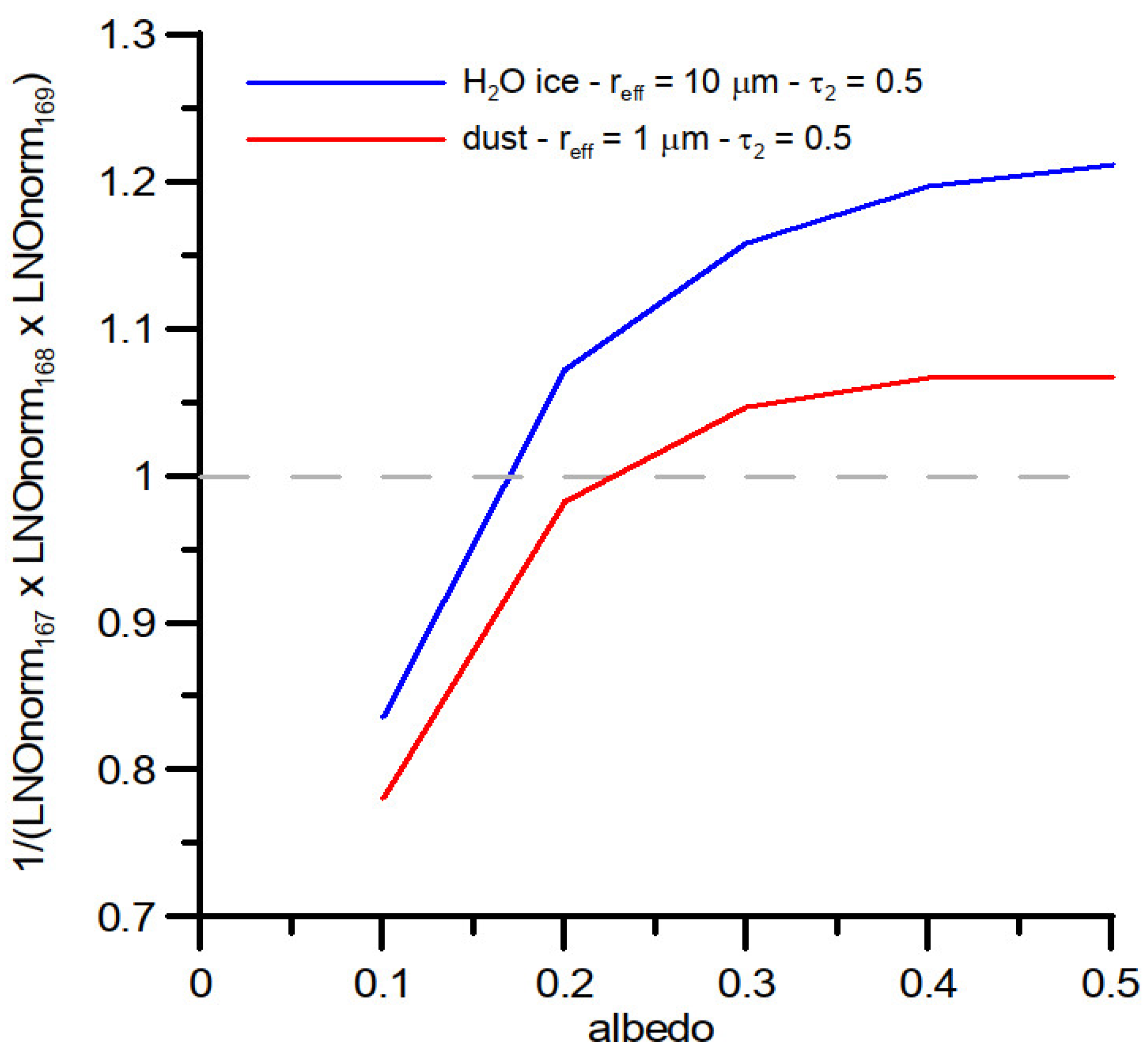
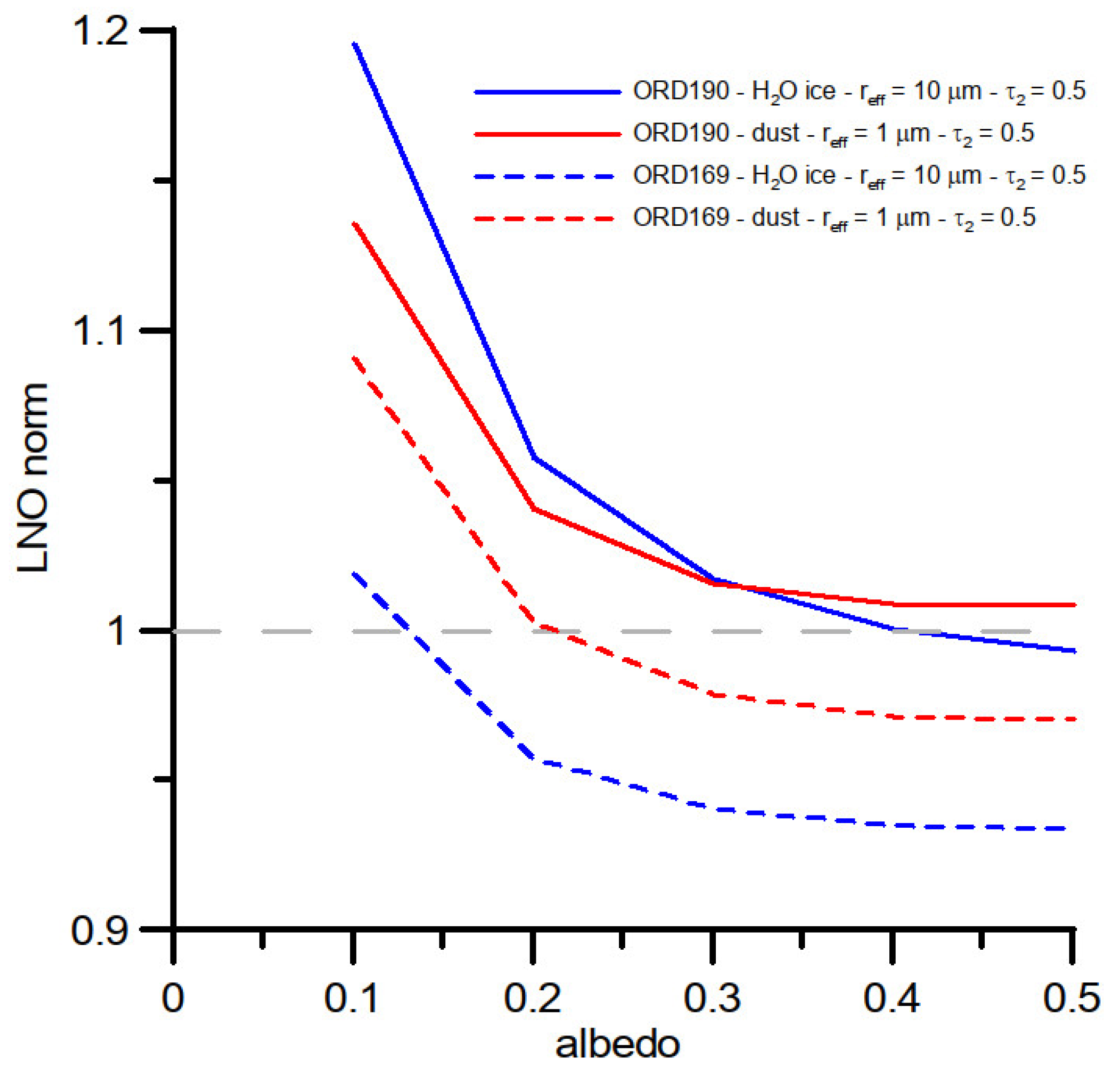
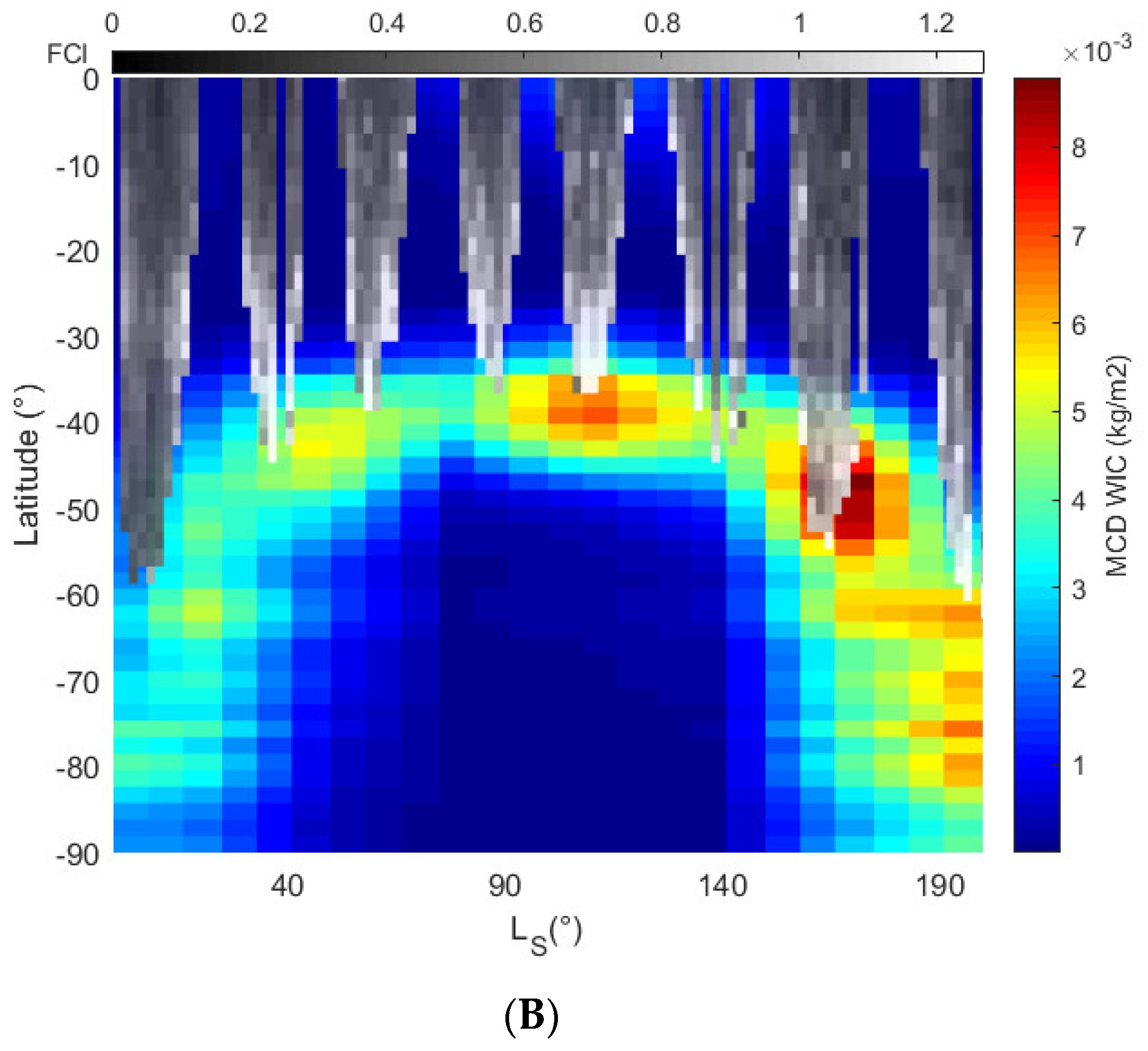
4.3. FCI Sensitivity

It is worth noting that the detections in region L are over low surface albedo regions covering Acidalia and Utopia Planitia [65]. As already mentioned in Section 4, the dark latitudinal band around 60°N affects the measured reflectance [18,52]. Therefore, we investigate in this section the possibility of having surface effects residues in the results of the region L (see Figure 6). We apply the FCI on observations between L_S 30° and 150° in MY35. In order to verify an eventual correlation between the FCI and the dark terrains, we can perform a direct comparison with the TES albedo map. The results are given in terms of latitude and longitude in Figure 8. As we can see, saturated values of the FCI (>3.5σ, see Section 4.1) are present over Acidalia Planitia and the north of that region (see red rectangle on the left panel). They can also be seen at the highest-probed latitudes in both hemispheres (see black circles on the left panel). These high index values should be related to the presence of water ice clouds (see Section 3.2 and Section 4.2). Nevertheless, by comparison with the right panel, we see that the high FCI values inside the red rectangle present a correlation with dark terrains. Since TES albedo is bolometric, the correlation we observe can result from an overestimation of albedo values over dark regions at 2.7 µm with respect to LNO. Therefore, the high values in the red rectangle (see left panel) are likely linked to the presence of surface effect residues over Acidalia Planitia in the LNO data. This is hence in agreement with the OMEGA results in Szantai et al. [18].

In Figure 8, the selected period corresponds to the aphelion season. The circles cover regions with an intermediate surface albedo. These regions are not comparable with dark regions in the northern high latitudes [65]. Therefore, the saturated FCI values in both hemispheres are likely linked to the presence of clouds. As highlighted in Section 4.2, the low WIC of the ACB makes its detection difficult in the LNO spectral range [10]. The full ACB structure is not hence visible. For that reason, we attempt to derive the FCI sensitivity limit for cloud detection. From MCD simulations, we notice that the PH water ice column can take values of the same order as those of the surface water ice (~10⁻² kg/m²). They are then superior by a factor 10 to those of the ACB (~10⁻³ kg/m²). However, the PH is not always fully detected (see region I in Figure 6). Moreover, some detections have been recorded around the equator during the Aphelion season (see the regions B–D in Figure 6). Local thick clouds in the ACB can hence be detected. In order to estimate the sensitivity limit of the FCI, we compare the FCI results in Figure 8 with the MCD predictions (see Figure 9). We can see that the WIC of the ACB takes values lower than 3 × 10⁻³ kg/m². In contrast, those in the centre of the SPH are generally higher than 5 × 10⁻³ kg/m², while the WIC of the NPH can reach 1.3 × 10⁻² kg/m². From the saturated index values at the highest latitudes (white pixels), we can estimate the limit of the FCI sensitivity for cloud detection at ~4 × 10⁻³ kg/m². Some saturated pixels are found at mid latitudes, which may indicate the presence of thicker clouds compared to the rest of the ACB (see black circle). Nevertheless, as over Acidalia Planitia (see red rectangle), we suspect a surface effect in the detection inside the yellow rectangle. Indeed, this region covers a terrain with a low surface albedo (TES albedo lower than 0.1, see Figure 8).

5. Conclusions

NOMAD-LNO is a spectrometre mainly designed to investigate the presence of trace gases in the Martian atmosphere. The instrument uses preselected spectral orders to resolve the absorption lines of the single species. Due to this mode of operations and to its high resolving power, it cannot acquire a single spectrum over the full spectral range (see Section 2). Therefore, the spatial coverage linked to the full spectral range is also limited, since each spectral order observes a different footprint. Moreover, due to technical constraints imposed by the spacecraft, the SNR is not optimal. Finally, there is an intrinsic limitation linked to the spectral behaviour of ice clouds and dust. Depending on their microphysical properties, it can be really challenging to distinguish between them. Having all these constraints and limitations in mind, we have described a technique that takes advantage of three NOMAD-LNO diffraction orders (167, 168, and 169), covering the short wavelength shoulder of the 2.7 μm ice absorption band. The application of such a technique allows us to map surface ice and H₂O ice clouds into the Martian atmosphere. We applied the method on regions where ice clouds are either expected by general circulation models or have been observed by other instruments. The method is based on spectral ratios between LNO reflectance factor spectra and TES bolometric dust-clean albedo. We have defined a Frost and Cloud Index (FCI) as a useful proxy for ice mapping (see Section 3). We applied the method to the LNO dataset in Martian years 34 and 35 (March 2018 to February 2021) excluding observations with SZA larger than 60° to avoid the lowest SNRs (see Section 4). As discussed in Section 4.2, the acquisition of data during MY34-35 allows us to construct seasonal maps for water ice clouds. The results appear in agreement with previous studies focused on Mars Express SPICAM/UV and OMEGA data analysis [10,17]. FCI is sensitive to the Polar Hood clouds, although the full structure is not detected. Moreover, detections in the Aphelion Cloud Belt (ACB) are limited. This is consistent with previous OMEGA observations [10] showing different physical properties between the two main Martian atmospheric structures and making the ACB less detectable in the infrared. We hence derived the LNO channel sensitivity limit for cloud detection (see Section 4.3).

Finally, the analysis presented in this paper represents one of several studies dedicated to the exploitation of the LNO nadir dataset and opens the way for different follow-up papers. As a direct continuation to this work, further comparison with the NOMAD-UVIS channel about the cloud’s detection is already planned. It will help to tune the FCI, hopefully to increase its sensitivity to ice clouds and to limit the number of false detections. In addition, an in-depth radiative transfer analysis of the 2.35 µm feature in CO₂ ice clouds spectra is currently being performed.

References

1. Langevin, Y.; Bibring, J.-P.; Montmessin, F.; Forget, F.; Vincendon, M.; Douté, S.; Poulet, F.; Gondet, B. Observations of the south seasonal cap of Mars during recession in 2004–2006 by the OMEGA visible/near-infrared imaging spectrometer on board Mars Express. J. Geophys. Res. 2007, 112, E08S12. [Google Scholar] [CrossRef]
2. Montmessin, F.; Gondet, B.; Bibring, J.-P.; Langevin, Y.; Drossart, P.; Forget, F.; Fouchet, T. Hyperspectral imaging of convective CO2 ice clouds in the equatorial mesosphere of Mars. J. Geophys. Res. Planets 2007, 112, E11S90. [Google Scholar] [CrossRef]
3. Clancy, R.T.; Wolff, M.J.; Christensen, P.R. Mars aerosol studies with the MGS TES emission phase function observations: Optical depths, particle sizes, and ice cloud types versus latitude and solar longitude. J. Geophys. Res. Planets 2003, 108. [Google Scholar] [CrossRef]
4. Clancy, R.T.; Wolff, M.J.; Smith, M.D.; Kleinböhl, A.; Cantor, B.A.; Murchie, S.L.; Toigo, A.D.; Seelos, K.; Lefèvre, F.; Montmessin, F.; et al. The distribution, composition, and particle properties of Mars mesospheric aerosols: An analysis of CRISM visible/near-IR limb spectra with context from near-coincident MCS and MARCI observations. Icarus 2019, 328, 246–273. [Google Scholar] [CrossRef]
5. Wolff, M.J.; Clancy, R.T. Constraints on the size of Martian aerosols from Thermal Emission Spectrometer observations. J. Geophys. Res. Planets 2003, 108. [Google Scholar] [CrossRef]
6. Smith, M.D. Interannual variability in TES atmospheric observations of Mars during 1999–2003. Icarus 2004, 167, 148–165. [Google Scholar] [CrossRef]
7. Smith, M.D.; Wolff, M.J.; Clancy, R.T.; Kleinböhl, A.; Murchie, S.L. Vertical distribution of dust and water ice aerosols from CRISM limb-geometry observations. J. Geophys. Res. Planets 2013, 118, 321–334. [Google Scholar] [CrossRef]
8. Liuzzi, G.; Villanueva, G.L.; Crismani, M.M.; Smith, M.D.; Mumma, M.J.; Daerden, F.; Aoki, S.; Vandaele, A.C.; Clancy, R.T.; Erwin, J.; et al. Strong variability of Martian water ice clouds during dust storms revealed from ExoMars Trace Gas Orbiter/NOMAD. J. Geophys. Res. Planets 2020, 125, e2019JE006250. [Google Scholar] [CrossRef]
9. Wolff, M.J.; Clancy, R.T.; Kahre, M.A.; Haberle, R.M.; Forget, F.; Cantor, B.A.; Malin, M.C. Mapping water ice clouds on Mars with MRO/MARCI. Icarus 2019, 332, 24–49. [Google Scholar] [CrossRef]
10. Olsen, K.S.; Forget, F.; Madeleine, J.-B.; Szantai, A.; Audouard, J.; Geminale, A.; Altieri, F.; Bellucci, G.; Oliva, F.; Montabone, L.; et al. Retrieval of the water ice column and physical properties of water-ice clouds in the Martian atmosphere using the OMEGA imaging spectrometer. Icarus 2021, 353, 113229. [Google Scholar] [CrossRef]
11. Clancy, R.; Grossman, A.; Wolff, M.; James, P.; Rudy, D.; Billawala, Y.; Sandor, B.; Lee, S.; Muhleman, D. Water vapor saturation at low altitudes around Mars aphelion: A key to mars climate? Icarus 1996, 122, 36–62. [Google Scholar] [CrossRef]
12. Smith, M.D. Spacecraft observations of the Martian atmosphere. Annu. Rev. Earth Planet. Sci. 2008, 36, 191–219. [Google Scholar] [CrossRef]
13. Smith, M.D. THEMIS observations of Mars aerosol optical depth from 2002–2008. Icarus 2009, 202, 444–452. [Google Scholar] [CrossRef]
14. Benson, J.L.; Kass, D.M.; Kleinböhl, A.; McCleese, D.J.; Schofield, J.T.; Taylor, F.W. Mars’ south polar hood as observed by the Mars Climate Sounder. J. Geophys. Res. Planets 2010, 115. [Google Scholar] [CrossRef]
15. Benson, J.L.; Kass, D.M.; Kleinböhl, A. Mars’ north polar hood as observed by the Mars Climate Sounder. J. Geophys. Res. Planets 2011, 116. [Google Scholar] [CrossRef]
16. Madeleine, J.B.; Forget, F.; Spiga, A.; Wolff, M.J.; Montmessin, F.; Vincendon, M.; Jouglet, D.; Gondet, B.; Bibring, J.P.; Langevin, Y.; et al. Aphelion water-ice cloud mapping and property retrieval using the OMEGA imaging spectrometer onboard Mars Express. J. Geophys. Res. 2012, 117, E00J07. [Google Scholar] [CrossRef]
17. Willame, Y.; Vandaele, A.; Depiesse, C.; Lefèvre, F.; Letocart, V.; Gillotay, D.; Montmessin, F. Retrieving cloud, dust and ozone abundances in the martian atmosphere using SPICAM/UV nadir spectra. Planet. Space Sci. 2017, 142, 9–25. [Google Scholar] [CrossRef]
18. Szantai, A.; Audouard, J.; Forget, F.; Olsen, K.S.; Gondet, B.; Millour, E.; Madeleine, J.B.; Pottier, A.; Langevin, Y.; Bibring, J.P. Martian cloud climatology and life cycle extracted from Mars Express OMEGA spectral images. Icarus 2021, 353, 114101. [Google Scholar] [CrossRef]
19. Wu, Z.; Li, T.; Heavens, N.G.; Newman, C.E.; Richardson, M.I.; Yang, C.; Li, J.; Cui, J. Earth-like thermal and dynamical coupling processes in the Martian climate system. Earth-Sci. Rev. 2022, 229, 104023. [Google Scholar] [CrossRef]
20. Benson, J.L.; Boney, B.P.; James, P.B.; Shan, K.J.; Cantor, B.A.; Caplinger, M.A. The seasonal behavior of water ice clouds in the Tharsis and Valles Marineris regions of Mars: Mars orbiter camera observations. Icarus 2003, 165, 34–52. [Google Scholar] [CrossRef]
21. Benson, J.L.; James, P.B.; Cantor, B.A.; Remigio, R. Interannual variability of water ice clouds over major Martian volcanoes observed by MOC. Icarus 2006, 184, 365–371. [Google Scholar] [CrossRef]
22. Hernández-Bernal, J.; Sánchez-Lavega, A.; del Río-Gaztelu Urrutia, T.; Ravanis, E.; Cardesín-Moinelo, A.; Connour, K.; Tirsch, D.; Ordóñez-Etxeberria, I.; Gondet, B.; Wood, S.; et al. An extremely elongated cloud over Arsia Mons volcano on Mars: I. Life cycle. J. Geophys. Res. Planets 2021, 126, e2020JE006517. [Google Scholar] [CrossRef]
23. Forget, F.; Pierrehumbert, R.T. Warming early Mars with carbon dioxide clouds that scatter infrared radiation. Science 1997, 278, 1273–1276. [Google Scholar] [CrossRef]
24. Forget, F.; Hourdin, F.; Talagrand, O. CO2 snowfall on Mars: Simulation with a general circulation model. Icarus 1998, 131, 302–316. [Google Scholar] [CrossRef]
25. Forget, F.; Hourdin, F.; Fournier, R.; Hourdin, C.; Talagrand, O.; Collins, M. Improved general circulation models of the Martian atmosphere from the surface to above 80 km. J. Geophys. Res. 1999, 104, 24155–24175. [Google Scholar] [CrossRef]
26. Richardson, M.I.; Wilson, R.J.; Rodin, A.V. Water ice clouds in the Martian atmosphere: General circulation model experiments with a simple cloud scheme. J. Geophys. Res. Planets 2002, 107. [Google Scholar] [CrossRef]
27. Montmessin, F.; Forget, F.; Rannou, P.; Cabane, M.; Haberle, R.M. Origin and role of water ice clouds in the Martian water cycle as inferred from a general circulation model. J. Geophys. Res. Planets 2004, 109, E10004. [Google Scholar] [CrossRef]
28. Navarro, T.; Madeleine, J.-B.; Forget, F.; Spiga, A.; Millour, E.; Montmessin, F.; Määttänen, A. Global Climate Modeling of the Martian water cycle with improved microphysics and radiatively active water ice clouds. J. Geophys. Res. Planets 2014, 119, 1479–1495. [Google Scholar] [CrossRef]
29. Daerden, F.; Whiteway, J.A.; Davy, R.; Verhoeven, C.; Komguem, L.; Dickin-son, C.; Taylor, P.A.; Larsen, N. Simulating observed boundary layer clouds on Mars. Geophys. Res. Lett. 2010, 37. [Google Scholar] [CrossRef]
30. Daerden, F.; Neary, L.; Viscardy, S.; Garcia, M.A.; Clancy, R.; Smith, M.; Encrenaz, T.; Fedorova, A. Mars atmospheric chemistry simulations with the GEM-Mars general circulation model. Icarus 2019, 326, 197–224. [Google Scholar] [CrossRef]
31. Aoki, S.; Vandaele, A.C.; Daerden, F.; Villanueva, G.L.; Liuzzi, G.; Thomas, I.R.; Erwin, J.T.; Trompet, L.; Robert, S.; Neary, L.; et al. Water vapor vertical profiles on Mars in dust storms observed by TGO/NOMAD. J. Geophys. Res. Planets 2019, 124, 3482–3497. [Google Scholar] [CrossRef]
32. Vandaele, A.C.; Korablev, O.; Daerden, F.; Aoki, S.; Thomas, I.R.; Altieri, F.; López-Valverde, M.; Villanueva, G.; Liuzzi, G.; Smith, M.D.; et al. Martian dust storm impact on atmospheric H2O and D/H observed by ExoMars Trace Gas Orbiter. Nature 2019, 568, 521–525. [Google Scholar] [CrossRef]
33. Liuzzi, G.; Villanueva, G.L.; Mumma, M.J.; Smith, M.D.; Daerden, F.; Ristic, B.; Thomas, I.; Vandaele, A.C.; Patel, M.R.; Lopez-Moreno, J.-J.; et al. Methane on Mars: New insights into the sensitivity of CH4 with the NOMAD/ExoMars spectrometer through its first in-flight calibration. Icarus 2019, 321, 671–690. [Google Scholar] [CrossRef]
34. Korablev, O.; Olsen, K.S.; Trokhimovskiy, A.; Lefèvre, F.; Montmessin, F.; Fedorova, A.A.; Toplis, M.J.; Alday, J.; Belyaev, D.A.; Patrakeev, A.; et al. Transient HCl in the atmosphere of Mars. Sci. Adv. 2021, 7, eabe4386. [Google Scholar] [CrossRef] [PubMed]
35. Smith, M.D.; Daerden, F.; Neary, L.; Khayat, A.S.; Holmes, J.A.; Patel, M.R.; Villanueva, G.; Liuzzi, G.; Thomas, I.R.; Ristic, B.; et al. The climatology of carbon monoxide on Mars as observed by NOMAD nadir-geometry observations. Icarus 2021, 362, 114404. [Google Scholar] [CrossRef]
36. Neefs, E.; Vandaele, A.C.; Drummond, R.; Thomas, I.R.; Berkenbosch, S.; Clairquin, R.; Delanoye, S.; Ristic, B.; Maes, J.; Bonnewijn, S.; et al. NOMAD spectrometer on the ExoMars Trace Gas Orbiter mission: Part1—Design, manufacturing and testing of the infrared channels. Appl. Opt. 2015, 54, 8494–8520. [Google Scholar] [CrossRef] [PubMed]
37. Vandaele, A.; Neefs, E.; Drummond, R.; Thomas, I.; Daerden, F.; Lopez-Moreno, J.-J.; Rodriguez, J.; Patel, M.; Bellucci, G.; Allen, M.; et al. Science objectives and performances of NOMAD, a spectrometer suite for the ExoMars TGO mission. Planet. Space Sci. 2015, 119, 233–249. [Google Scholar] [CrossRef]
38. Vandaele, A.C.; Willame, Y.; Depiesse, C.; Thomas, I.R.; Robert, S.; Bolsée, D.; Patel, M.R.; Mason, J.P.; Leese, M.; Lesschaeve, S.; et al. Optical and radiometric models of the nomad instrument part I: The UVIS channel. Opt. Express 2015, 23, 30028–30042. [Google Scholar] [CrossRef]
39. Thomas, I.R.; Vandaele, A.; Robert, S.; Neefs, E.; Drummond, R.; Daerden, F.; Delanoye, S.; Ristic, B.; Berkenbosch, S.; Clairquin, R. Optical and radiometric models of the NOMAD instrument part II: The infrared channels-SO and LNO. Opt. Express 2016, 24, 3790–3805. [Google Scholar] [CrossRef]
40. Patel, M.R.; Antoine, P.; Mason, J.P.; Leese, M.R.; Hathi, B.; Stevens, A.H.; Dawson, D.; Gow, J.P.D.; Ringrose, T.J.; Holmes, J.A.; et al. NOMAD spectrometer on the ExoMars Trace Gas Orbiter mission: Part 2—Design, manufacturing, and testing of the ultraviolet and visible channel. Appl. Opt. 2017, 56, 2771–2782. [Google Scholar] [CrossRef]
41. Thomas, I.R.; Shohei, A.; Trompet, L.; Robert, S.; Depiesse, C.; Willame, Y.; Cruz-Mermy, G.; Schmidt, F.; Erwin, J.T.; Vandaele, A.C.; et al. Calibration of NOMAD on ESA’s ExoMars Trace Gas Orbiter: Part 2—The Limb, Nadir and Occultation (LNO) channel. Planet. Space Sci. 2022, 218, 105410. [Google Scholar] [CrossRef]
42. Cruz Mermy, G.; Schmidt, F.; Thomas, I.R.; Daerden, F.; Ristic, B.; Patel, M.R.; Lopez-Moreno, J.J.; Bellucci, G.; Vandaele, A.C. Calibration of NOMAD on ExoMars Trace Gas Orbiter: Part 3—LNO validation and instrument stability. Planet. Space Sci. 2022, 218, 105399. [Google Scholar] [CrossRef]
43. Oliva, F.; D’Aversa, E.; Bellucci, G.; Carrozzo, F.G.; Ruiz Lozano, L.; Altieri, F.; Thomas, I.R.; Karatekin, O.; Cruz Mermy, G.; Schmidt, F.; et al. Martian CO2 ice observation at high spectral resolution with ExoMars/TGO NOMAD. J. Geophys. Res. Planets 2022, 127, e2021JE007083. [Google Scholar] [CrossRef]
44. Adriani, A.; Moriconi, M.; D’Aversa, E.; Oliva, F.; Filacchione, G. Faint luminescent ring over Saturn’s polar hexagon. Astrophys. J. Lett. 2015, 808, L16. [Google Scholar] [CrossRef]
45. Sindoni, G.; Grassi, D.; Adriani, A.; Mura, A.; Moriconi, M.; Dinelli, B.; Filac-chione, G.; Tosi, F.; Piccioni, G.; Migliorini, A.; et al. Characterization of the white ovals on Jupiter’s southern hemisphere using the first data by the JUNO/JIRAM instrument: Jupiter ovals as seen by JIRAM/JUNO. Geophys. Res. Lett. 2017, 44, 4660–4668. [Google Scholar] [CrossRef]
46. Oliva, F.; Adriani, A.; Moriconi, M.; Liberti, G.L.; D’Aversa, E.; Filacchione, G. Clouds and hazes vertical structure of a Saturn’s giant vortex from Cassini/VIMS-V-v data analysis. Icarus 2016, 278, 215–237. [Google Scholar] [CrossRef]
47. Oliva, F.; Geminale, A.; D’Aversa, E.; Altieri, F.; Bellucci, G.; Carrozzo, F.; Sindoni, G.; Grassi, D. Properties of a Martian local dust storm in Atlantis chaos from OMEGA/MEX data. Icarus 2018, 300, 1–11. [Google Scholar] [CrossRef]
48. Mayer, B.; Kylling, A. Technical note: The libRadtran software package for radiative transfer calculations? Description and examples of use. Atmos. Chem. Phys. Discuss. 2005, 5, 1319–1381. [Google Scholar] [CrossRef]
49. Christensen, P.R.; Bandfield, J.L.; Hamilton, V.E.; Ruff, S.W.; Kieffer, H.H.; Titus, T.N.; Malin, M.C.; Morris, R.V.; Lane, M.D.; Clark, R.L.; et al. Mars Global Surveyor Thermal Emission Spectrometer experiment: Investigation description and surface science results. J. Geophys. Res. Planets 2001, 106, 23823–23872. [Google Scholar] [CrossRef]
50. Bibring, J.P.; Soufflot, A.; Berthé, M.; Langevin, Y.; Gondet, B.; Drossart, P.; Buoyé, M.; Combes, M.; Puget, P.; Semery, A.; et al. OMEGA: Observatoire Pour La Minéralogie, l’Eau, Les Glaces et l’Activité. In Mars Express: The Scientific Payload; Wilson, A., Chicarro, A., Eds.; European Space Agency: Paris, France, 2004; Volume 1240, pp. 37–49. [Google Scholar]
51. Murchie, S.; Arvidson, R.; Bedini, P.; Beisser, K.; Bibring, J.-P.; Bishop, J.; Boldt, J.; Cavender, P.; Choo, T.; Clancy, R.T.; et al. Compact Reconnaissance Imaging Spectrometer for Mars (CRISM) on Mars Reconnaissance Orbiter (MRO). J. Geophys. Res. Planets 2007, 112. [Google Scholar] [CrossRef]
52. Viviano, C.E.; Seelos, F.P.; Murchie, S.L.; Kahn, E.G.; Seelos, K.D.; Taylor, H.W.; Taylor, K.; Ehlmann, B.L.; Wiseman, S.M.; Mustard, J.F.; et al. Revised CRISM spectral parameters and summary products based on the currently detected mineral diversity on Mars. J. Geophys. Res. Planets 2014, 119, 1403–1431. [Google Scholar] [CrossRef]
53. Riu, L.; Poulet, F.; Carter, J.; Bibring, J.-P.; Gondet, B.; Vincendon, M. The M3 project: 1—A global hyperspectral image-cube of the Martian surface. Icarus 2019, 319, 281–292. [Google Scholar] [CrossRef]
54. Riu, L.; Poulet, F.; Bibring, J.-P.; Gondet, B. The M3 project: 2—Global distributions of mafic mineral abundances on Mars. Icarus 2019, 322, 31–53. [Google Scholar] [CrossRef]
55. Christensen, P.; Bandfield, J.L.; Hamilton, V.E.; Howard, D.A.; Lane, M.D.; Piatek, J.L.; Ruff, S.; Stefanov, W.L. A thermal emission spectral library of rock-forming minerals. J. Geophys. Res. Planets 2000, 105, 9735–9739. [Google Scholar] [CrossRef]
56. Poulet, F.; Mangold, N.; Platevoet, B.; Bardintzeff, J.M.; Sautter, V.; Mustard, J.F.; Bibring, J.P.; Pinet, P.; Langevin, Y.; Gondet, B.; et al. Quantitative compositional analysis of Martian mafic regions using the MEx/OMEGA reflectance data: 2. Petrological implications. Icarus 2009, 201, 84–101. [Google Scholar] [CrossRef]
57. Piqueux, S.; Byrne, S.; Richardson, M.I. Sublimation of Mars’s southern seasonal CO2 ice cap and the formation of spiders. J. Geophys. Res. 2003, 108, 5084. [Google Scholar] [CrossRef]
58. Schmidt, F.; Douté, S.; Schmitt, B.; Vincendon, M.; Bibring, J.-P.; Langevin, Y.; OMEGA Team. Albedo control of Seasonal South Polar Cap recession on Mars. Icarus 2009, 200, 374–394. [Google Scholar] [CrossRef]
59. Schmidt, F.; Schmitt, B.; Douté, S.; Forget, F.; Jian, J.J.; Martin, P.; Langevin, Y.; Bibring, J.P.; OMEGA Team. Sublimation of the Martian CO2 Seasonal South Polar Cap. Planet. Space Sci. 2010, 58, 1129–1138. [Google Scholar] [CrossRef]
60. Cull, S.; Arvidson, R.E.; Mellon, M.; Wiseman, S.; Clark, R.; Titus, T.; Morris, R.V.; McGuire, P. Seasonal H2O and CO2 ice cycles at the Mars Phoenix landing site: 1. Prelanding CRISM and HiRISE observations. J. Geophys. Res. 2010, 115, E00D16. [Google Scholar] [CrossRef]
61. Hansen, C.J.; Byrne, S.; Portyankina, G.; Bourke, M.; Dundas, C.; McEwen, A.; Mellon, M.; Pommerol, A.; Thomas, N. Observations of the northern seasonal polar cap on Mars: I. Spring sublimation activity and processes. Icarus 2013, 225, 881–897. [Google Scholar] [CrossRef]
62. Bandfield, J.L.; Christensen, P.R.; Smith, M.D. Spectral data set factor analysis and end-member recovery: Application to Martian atmospheric particulates. J. Geophys. Res. 2000, 105, 9573–9588. [Google Scholar] [CrossRef]
63. Bandfield, J.L. Global mineral distributions on Mars. J. Geophys. Res. 2002, 107. [Google Scholar] [CrossRef]
64. Rogers, D.; Christensen, P.R. Age relationship of basaltic and andesitic surface compositions on Mars: Analysis of high-resolution TES observations of the northern hemisphere. J. Geophys. Res. 2003, 108, 5030. [Google Scholar] [CrossRef]
65. Rogers, A.D.; Bandfield, J.L.; Christensen, P.R. Global spectral classification of Martian low-albedo regions with Mars Global Surveyor Thermal Emission Spectrometer (MGS-TES) data. J. Geophys. Res. 2007, 112, E02004. [Google Scholar] [CrossRef]
66. Piqueux, S.; Kleinböhl, A.; Hayne, P.O.; Heavens, N.G.; Kass, D.M.; McCleese, D.J.; Schofield, J.T.; Shirley, J.H. Discovery of a widespread low-latitude diurnal CO2 frost cycle on Mars. J. Geophys. Res. Planets 2016, 121, 1174–1189. [Google Scholar] [CrossRef]
67. Carrozzo, F.G.; Bellucci, G.; Altieri, F.; D’aversa, E.; Bibring, J.P. Mapping of water frost and ice at low latitudes on Mars. Icarus 2009, 203, 406–420. [Google Scholar] [CrossRef]
68. Millour, E.; Forget, F.; Spiga, A. The Mars Climate Database, Version 5.3; ESAC: Madrid, Spain, 2018. [Google Scholar]
69. Wilson, R.J.; Neumann, G.A.; Smith, M.D. Diurnal variation and radiative influence of Martian water ice clouds. Geophys. Res. Lett. 2007, 34, L02710. [Google Scholar] [CrossRef]
70. Guha, B.K.; Jagabandhu, P.; Zhaopeng, W. Observation of aphelion cloud belt over Martian tropics, its evolution, and associated dust distribution from MCS data. Adv. Space Res. 2021, 67, 1392–1411. [Google Scholar] [CrossRef]
71. Liu, J.; Richardson, M.I.; Wilson, R.J. An assessment of the global, seasonal, and interannual spacecraft record of Martian climate in the thermal infrared. J. Geophys. Res. 2003, 108, 5089. [Google Scholar] [CrossRef]
72. Mateshvili, N.; Fussen, D.; Vanhellemont, F.; Bingen, C.; Dodion, J.; Montmessin, F.; Perrier, S.; Dimarellis, E.; Bertaux, J.-L. Martian ice cloud distribution obtained from SPICAM nadir UV measurements. J. Geophys. Res. 2007, 112, E07004. [Google Scholar] [CrossRef]
73. Guzewich, S.D.; Smith, M.D. Seasonal Variation in Martian Water Ice Cloud Particle Size. J. Geophys. Res. Planets 2019, 124, 636–643. [Google Scholar] [CrossRef]
74. Clancy, R.T.; Wolff, M.J.; Whitney, B.A.; Cantor, B.A.; Smith, M.D. Mars equatorial mesospheric clouds: Global occurrence and physical properties from Mars Global Surveyor Thermal Emission Spectrometer and Mars Orbiter Camera limb observations. J. Geophys. Res. Planets 2007, 112, E04004. [Google Scholar] [CrossRef]
75. Clancy, T.R.; Wolff, M.J.; Heavens, N.G.; James, P.B.; Lee, S.W.; Sandor, B.J.; Cantor, B.A.; Malin, M.C.; Tyler, D.; Spiga, A. Mars perihelion cloud trails as revealed by MARCI: Mesoscale topographically focused updrafts and gravity wave forcing of high altitude clouds. Icarus 2021, 362, 114411. [Google Scholar] [CrossRef]
Figure 1. Simulated ice and dust spectra in the 2–2.8 µm range obtained by the MITRA tool [44,45,46,47]. The simulations have been performed with the following characteristics: a surface albedo of 0.2 (A = 0.2), an incidence angle of 0° (i = 0°), and an optical depth at 2 µm of 0.5 (τ2 = 0.5). We describe all aerosol layers by adopting lognormal size distributions with an effective variance of 0.1 (veff = 0.1) and characteristic grain sizes (reff). Vertical dashed lines indicate the centres of orders. See the legend on the panel for the colour definition.
Remotesensing 14 04143 g001
Figure 2. Simulated LNONorm vs. arbitrary albedo obtained by the MITRA tool. The simulations have been performed for water ice and dust using orders 190 and 169. See the legend on the panel for the colour definition.
Remotesensing 14 04143 g002
Figure 3. Simulated FCI vs. arbitrary albedo obtained by the MITRA tool. The simulations have been performed for water ice (in blue) and dust (in red) using orders 167, 168 and 169.
Remotesensing 14 04143 g003
Figure 4. Latitudinal-seasonal map of FCI. Observations cover MY34, from LS = 150° to 360°, and all MY35.
Remotesensing 14 04143 g004
Figure 5. FCI values distribution in logarithmic X-scale for MY34-35. Solid black line: mean value of the distribution (µ = −0.35). Dashed black line: standard deviation of the distribution (σ = 0.13). Dashed red line: mean value of FCI at the polar cap edge (µ + 3.5σ). Dashed blue line: mean value of FCI on the polar cap deposits (µ + 10σ).
Remotesensing 14 04143 g005
Figure 6. Latitudinal-seasonal maps of FCI. Observations cover MY34, from LS = 150° to 360°, and all MY35. (A) Yellow and red points indicate a FCI value above 3.5σ. The regions 1, 2 and, 3 in red correspond to the expected boundaries of the polar caps. The letters define regions of interest for cloud detection in yellow. (B) Colour points indicate the corresponding LTST.
Remotesensing 14 04143 g006
Figure 7. Comparison between the latitudinal-seasonal map of FCI (grey scale) with the one of MCD Water Ice Column (colour scale) for latitudes from 0° to 90°S and LS 0° to 200°. Grey scale: FCI results in region N (see Figure 6). Saturated FCI values are in white (>3.5σ, see Section 4.1). Colour scale: MCD Water ice column at 9 LTST (A), and 13 LTST (B).
Remotesensing 14 04143 g007aRemotesensing 14 04143 g007b
Figure 8. Left panel: LNO observations in MY35, from LS = 30° to 150°. Colour points indicate the FCI values saturated at 3.5σ (see Section 4.1). Right panel: TES albedo values falling in each bin of the LNO tracks in MY35, from LS = 30° to 150°. Red rectangle: correlation between high FCI values and region of low surface albedo. Black circle: example of high FCI values not correlated with regions of low surface albedo.
Remotesensing 14 04143 g008
Figure 9. Comparison between the FCI results (grey scale) with the MCD Water Ice Column (colour scale) for all latitudes and longitude from 100°W to 0°. Grey scale: LNO observations in MY35, from LS 30° to 150°. Saturated FCI values are in white (>3.5σ, see Section 4.1). Colour scale: MCD Water ice column simulation for LS 150° and 15 LTST.
Remotesensing 14 04143 g009