What You See Is What You Breathe? Estimating Air Pollution Spatial Variation Using Street-Level Imagery

Abstract

High spatial resolution information on urban air pollution levels is unavailable in many areas globally, partially due to the high input data needs of existing estimation approaches. We introduced a computer vision method to estimate annual means for air pollution levels from street-level images. We used annual mean estimates of NO₂ and PM_2.5 concentrations from locally calibrated models as labels from London, New York, and Vancouver to allow for compilation of a sufficiently large dataset (~250 k images for each city). Our experimental setup is designed to quantify intra- and intercity transferability of image-based model estimates. Performances were high and comparable to traditional land-use regression (LUR) and dispersion models when training and testing images from the same city (R² values between 0.51 and 0.95 when validated on data from ground monitoring stations). Similar to LUR models, transferability of models between cities in different geographies is more difficult. Specifically, transferability between the three cities (London, New York, and Vancouver), which have similar pollution source profiles, was moderately successful (R² values between zero and 0.67). Comparatively, performances when transferring models trained on cities with very different source profiles, such as Accra in Ghana and Hong Kong, were lower (R² between zero and 0.21). This suggests a need for local calibration, using additional measurement data from cities that share similar source profiles.

1. Introduction

Air pollution has significant and widely accepted implications on health outcomes [1,2,3,4]. Advances in spatial estimation of air pollution concentrations have been instrumental in establishing health effects and the impact of the burden of disease [5,6]. Yet, we currently lack information on air pollution levels in many areas globally [7], especially at sufficiently high spatial resolution, to inform local planning and air quality management strategies. The limited number of spatial and temporal resolution of air quality models partially results from input data requirements of existing estimation approaches; this includes physical based models such as dispersion models, and geostatistical models such as land use regression (LUR) models [8]. High quality air pollution measurements from ground measurement campaigns are required for development and calibration of city-wide air pollution models, yet they are very costly to implement and therefore not available to most cities around the world. Advances in deep learning methods and their success in computer vision applications has led to a growing interest in using images for estimating air pollution levels [8,9,10,11,12,13,14,15,16]. The rationale behind this interest is that information on pollution sources and common predictor variables used in traditional approaches (for example, land use, traffic, and built and natural environment features [17]) is, at least partially, visible from street-level and satellite images. If utilized effectively, this approach has the potential to reduce input data requirements and scale up to global coverage at a low cost.

Increasing the availability of images in cities makes the extraction of visual information at high spatial resolution feasible. In contrast, spatially detailed air pollutant concentration levels are typically not readily available. This is a substantial challenge in the application of deep learning methods, as they require very large numbers of labeled data (i.e., images and their corresponding air pollution levels) for training. One proposed solution [9,13,16,18] is to collect images when conducting air pollution monitoring campaigns. However, such data are rarely available and are costly to collect at the scale necessary for generalizing unseen locations. A second approach is to extract intermediate user defined features from images that are known to be important predictors of air pollution (e.g., trees, buildings, cars, buses, and roads) and to use them as explanatory variables to estimate pollutant levels with traditional regression methods [16]. This process, however, requires separate training on databases that may not contain crucial categories of interest or be publicly available. Furthermore, deep learning methods that automatically learn relevant features commonly outperform methods based on hand-crafted features in visual recognition tasks [19]. In this study, we propose a third approach, to estimate pollution levels from raw images without extracting intermediate user defined features. As the numbers of monitoring locations (in hundreds) from ground measurement campaigns are insufficient for training deep learning models, we propose to use annual mean estimates of air pollutant concentrations from locally calibrated models as labels for training. These local models provide continuous surfaces of pollution estimates at high spatial resolution. Use of LUR or dispersion-based estimates, matched with street-level images, allows for compilation of a large dataset of image-label pairs required for training deep learning models. Different types of images (e.g., street-level, aerial, and satellite images) will contain visual information captured from different viewpoints. Local information, especially near-road, (e.g., cars, building heights, and built and natural environmental features) is more visible from street images, while high resolution satellite and aerial images will contain more information on the spatial context (e.g., proximity to parks, forests, and oceans that are not necessarily visible from street level) [20]. Here, we use street-level images only to test whether locally rich information can be used to estimate spatial variation at high resolution. Variation of NO₂ is higher and is influenced more by local sources, likely visible from street images. On the other hand, PM_2.5 is influenced by regional levels and secondary production, which is less likely to be visible from street images. LUR models, for NO₂ especially, indicate that the variables describing the near-road environment explain much of the spatial variability within urban areas, and we hypothesize that street-level imagery would be useful in NO₂ modelling, but less relevant for estimation of variability in PM_2.5. However, while overall variability is harder to explain for PM_2.5, some can be explained by near-road predictors; we hypothesize that imagery may provide a richer dataset for estimation than geospatial predictors that have been identified previously.

In this study, we describe the application of a deep learning approach to estimate air pollution spatial variation using street-level images for PM_2.5 and NO₂. Our deep learning models work by automatically learning visual features associated with different levels of pollution to describe variation over space. These features may correspond to sources of pollution or pollution haze when visible from street images. First, we tested how transferable (i.e., similar) these visual features are within (intracity) and across (intercity) cities where we had good data from city-wide models and ground monitoring stations. For training the models, we used annual mean NO₂ and PM_2.5 estimates from three cities in three different countries, selected for their varying levels of pollution and the availability of high-resolution concentration estimates: London (UK), New York (USA), and Vancouver (Canada) [21,22,23,24,25,26]. A disadvantage of this approach, however, is that the performance of the image-based models will be influenced by the performance of the source models, the outputs of which were treated as the truth during the training phase. We used previously published models from all three cities and we included their performances against measured concentrations. Second, we made estimates for two additional large cities (Accra (Ghana) and Hong Kong (PRC)) as examples of locations where spatially resolved ground measurements are available. In Accra and Hong Kong, our estimates were based merely on street-level images with no additional information on the spatial context (such as regional pollution levels or proximity to parks or the ocean). Our selection of cities from different geographies, countries, and source profiles was deliberate, as it made the task of transferability particularly difficult. This means that we can better understand the transferability capabilities of image-based models in three different settings that vary in their level of expected difficulty for transferability performance: within the same city and country, across cities with similar source profiles but in different countries and geographies, and across cities with different source profiles and different geographies.

2. Materials and Methods

2.1. Land Use Regression and Dispersion Model Outputs

We obtained the annual mean estimates of NO₂ (200 m resolution raster) and PM_2.5 (100 m resolution raster) for 2010 from 3 cities (London, New York, and Vancouver) using the most recent local models developed for these cities [21,22,23,24,25,26,27,28]. Land use regression (LUR) models were available for New York and Vancouver and an atmospheric dispersion model for London. Land use regression and dispersion models are the 2 main model types used for estimating spatial variability, and we selected 3 cities where we had access to images and high-resolution annual estimates for both pollutants. We had access to a maintained dispersion model for London; however, there is no recent LUR for London for both pollutants. For other cities, LUR models were used and were available to us. The New York LUR models (r = 0.69 for PM_2.5 and r = 0.79 for NO₂, computed using ground measurements) included traffic density, proximity to bus routes, percentage of impervious surface, interior building space, proximity to industrial sites, and proximity to heat and hot water boilers as geospatial predictor variables. For Vancouver (r = 0.33 for PM_2.5 and r = 0.86 for NO₂) the model included vehicle density, proximity to commercial areas, elevation, and population density as predictor variables. The model in London (r = 0.65 for PM_2.5 and r = 0.49 for NO₂) used distance to roads by type, street canyon type, and meteorological inputs as key input variables. Distributions of annual estimates for both pollutants were distinct and almost non-overlapping for each of the study cities (Figure 1). The differences in absolute levels of pollution across cities is by design for our experiment and makes intercity transferability challenging, as discussed in Section 3. NO₂ estimates demonstrated a clear spatial trend following roads as the main source, whereas PM_2.5 levels are more heterogeneously spread, reflecting the diversity of sources, the impact of regional factors, and secondary production (Figure 2). Vancouver is characterized by low levels of NO₂ and PM_2.5 concentrations. Areas near downtown and the Vancouver International Airport show relatively higher levels of air pollution, whereas large parks and mountainous areas have low pollution levels (Figure 2). This resulted in bimodal distribution for both PM_2.5 and NO₂ in Vancouver, with a distinct local peak at the lower end in Figure 1. A similar bimodal distribution was observed in New York, especially for NO₂, whereas London estimates showed unimodal distributions for both pollutants. Both New York and London are right skewed. In New York, densely populated Manhattan, as well as Queens and Brooklyn Heights, stand out with their high levels of pollution. In London, similarly, the densely populated city center, as well as areas near major roads, have high levels of pollution. London contained the highest estimates for both pollutants.

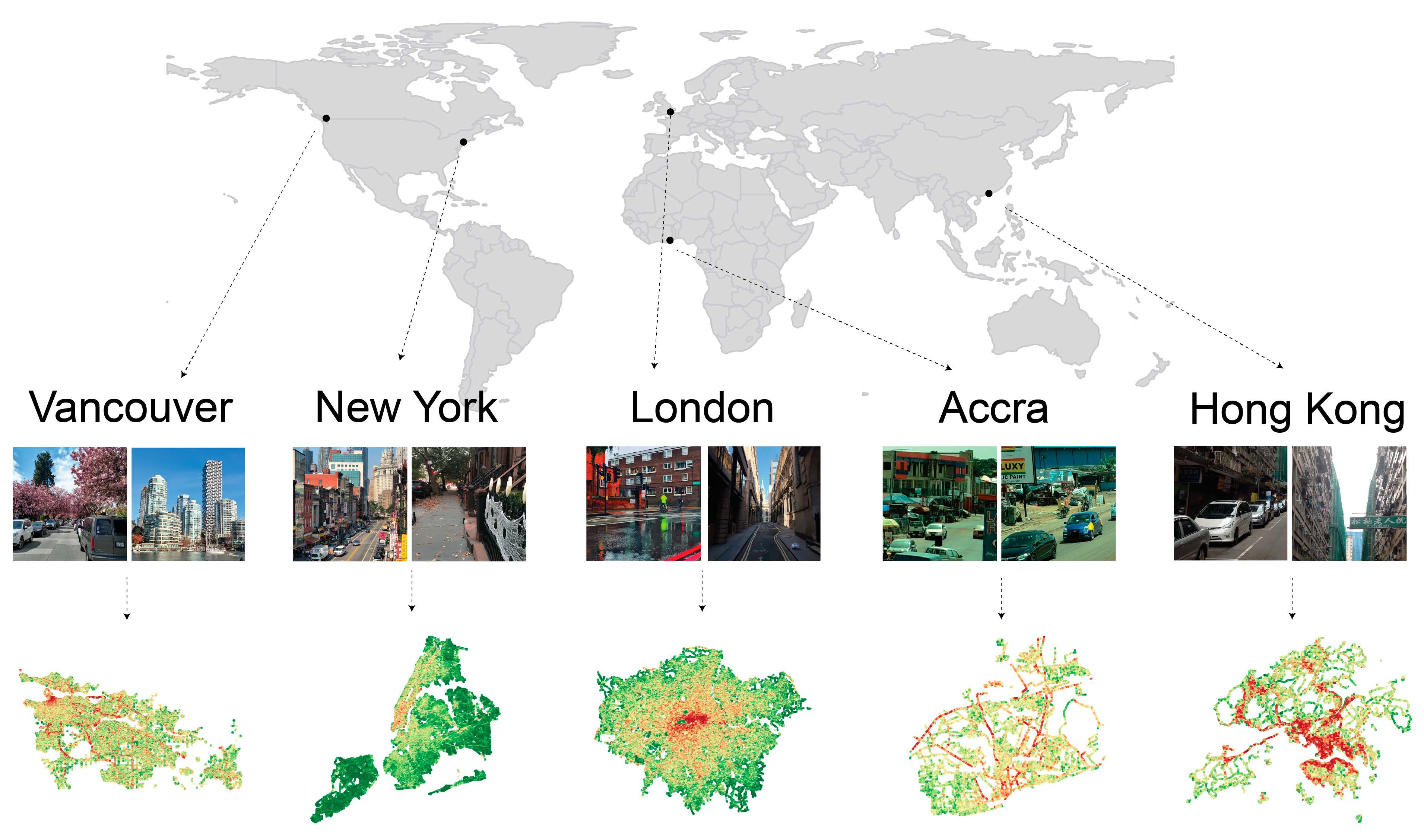
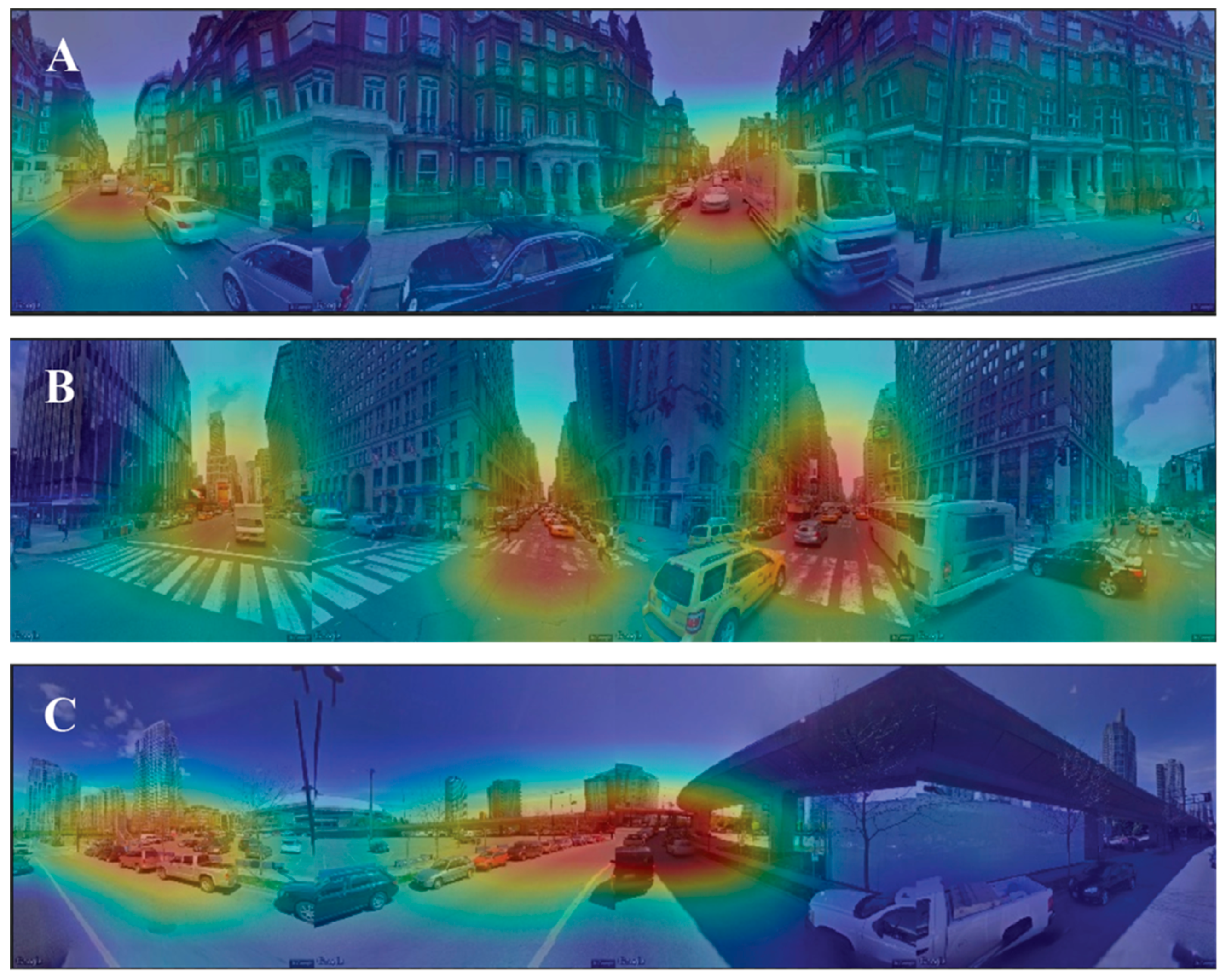
2.2. Street-Level Images

To obtain images, a 100 m grid for London, New York, and Vancouver was created using the boundary shape files covering the model output domains. Grids of 100 m for Accra and Hong Kong were created using the city boundary shape files. For each of the grid centroid points, we used the nearest street-level panorama image location available from Google Street View that was captured from 2008 to 2012 (±2 years from the model year) for London, New York, and Vancouver. For each image location, 4 images of 224 × 224 pixels were accessed, specifying the camera direction (i.e., 0°, 90°, 180°, and 270°) relative to the street view vehicle to cover a 360° view. These images were then concatenated, resulting in a single image of 224 × 896 pixels used as an input to the network as explained in Section 2.4. Nearly 820,000 street-level images (378,856 images for London, 198,300 for New York, and 242,248 for Vancouver) were matched with NO₂ and PM_2.5 model estimates (see Section 2.1) as outcome labels. For Accra and Hong Kong, we obtained the most recent panorama image for each of the grid centroid points corresponding to the years 2018 and 2019, resulting in a total of 250,460 and 265,308 images, respectively.

2.3. Ground Monitoring Stations

Site measurement data were obtained from ground-based air monitoring stations from each of the 3 study cities for evaluating the image-based air pollution estimates. More information about stations and data collection protocols used are available from [23,29,30,31,32]. Stations were included for evaluations where a street image (and consequently an image-based estimate) was available within 50 m. For London, daily station data from [31] was used to calculate the annual means of measured pollution over ground stations that had at least 1 measured value every month for 2010. For Vancouver and New York, annual means of measured data from [23,29,30,32] were used for stations that had collected data for more than half of the year during 2010. We used a total of 59 ground NO₂ sites with 8, 4, and 47 sites in London, New York, and Vancouver, respectively. For PM_2.5, a total of 15 stations were used with 9, 2, and 4 sites, respectively. London had the highest average pollutant values for NO₂ and PM_2.5 (63.4 and 16.3 µg/m³, respectively) followed by New York (54.1 and 11.3 µg/m³) and Vancouver, with the lowest (11.0 and 4.0 µg/m³) levels. Unfortunately, the numbers of available ground monitoring stations were very low. More data from ground monitoring stations are needed for evaluations to generalize our analysis from comparisons between image-based predictions and ground truth measurements. We report our findings in the following section.

The metrics used for evaluations in

Table 1. Summary of model performances for all experiments.

			City-Wide LUR Based Estimates of Air Pollution
			London					New York					Vancouver
		r	RMSE	NRMSE	R2	ME	r	RMSE	NRMSE	R2	ME	r	RMSE	NRMSE	R2	ME
NO2			N = 94,714					N = 49,575					N = 60,562
Intracity		0.79	7.31	0.20	0.62	−0.19	0.87	3.83	0.18	0.75	0.34	0.73	1.81	0.19	0.52	0.11
Intercity		0.42	21.38	0.58	0.18	18.80	0.60	12.83	0.59	0.36	−8.66	0.28	17.57	1.81	0.08	−16.69
Adj. intercity			12.07	0.32		0.00		6.89	0.31		0.00		3.12	0.32		0.00
PM2.5
Intracity		0.79	0.88	0.06	0.59	0.04	0.85	0.61	0.06	0.71	0.069	0.60	1.63	0.49	0.33	0.14
Intercity		0.37	5.77	0.40	0.14	5.52	0.47	4.06	0.42	0.22	−2.21	0.06	9.10	2.73	0.00	−8.80
Adj. intercity			1.55	0.11		0.00		1.17	0.12		0.00		2.75	0.82		0.00
			Ground Monitoring Stations
			London					New York					Vancouver
		r	RMSE	NRMSE	R2	ME	r	RMSE	NRMSE	R2	ME	r	RMSE	NRMSE	R2	ME
NO2			N = 8					N = 47					N = 4
Intracity		0.90	17.71	0.27	0.81	13.47	0.76	27.97	0.49	0.58	26.29	0.97	2.63	0.24	0.95	1.65
Intercity		0.82	46.22	0.71	0.67	41.91	0.51	22.30	0.39	0.26	17.90	0.51	13.70	1.23	0.00	−12.14
Adj. intercity			13.52	0.21		0.00		14.38	0.25		0.00		4.81	0.43		0.00
PM2.5			N = 9					N = 4					N = 2
Intracity		0.72	2.19	0.13	0.51	−0.34	0.86	1.15	0.10	0.74	1.56	-	1.04	0.25	-	0.70
Intercity		0.46	8.03	0.48	0.22	7.54	0.29	5.26	0.47	0.09	−4.41	-	8.81	2.15	-	−8.7
Adj. intercity			2.72	0.16		0.00		0.65	0.06		0.00		0.78	0.19		0.00
			Hong Kong					Accra
		r	RMSE	NRMSE	R2	ME	r	RMSE	NRMSE	R2	ME
NO2			N = 97					N = 35
Intercity		0.46	63.30	0.58	0.21	51.63	0.25	38.55	0.63	0.06	30.19
Adj. intercity			42.42	0.39		0.00		28.65	0.47		0.00
PM2.5			N = 52					N = 32
Intercity		0.02	8.35	0.36	0.00	3.90	−0.12	13.02	0.61	0.01	8.09
Adj. intercity			9.76	0.42		0.00		11.91	0.56		0.00

ME and RMSE values are reported in µg/m³.

need to be interpreted carefully for cities with small numbers of ground station data. Ground monitoring station data offered an evaluation based upon a measured (ground truth) dataset in addition to the evaluations undertaken on modelled data. Since the models developed for New York, Vancouver, and London were not calibrated using ground monitoring station data, these measurements can be used as an independent test set for these cities. We used ground measurement data from Accra and Hong Kong, collected through previous spatial monitoring field campaigns. For Hong Kong, we used data from 97 NO₂ sites and 52 PM_2.5 sites collected in 2014 as detailed elsewhere [33]. For Accra, data was available from 35 NO₂ sites and 32 PM_2.5 sites collected from 2019 to 2020 [18,34,35].

2.4. Modelling Approach

We used ResNet [36] architecture, where outputs are continuous pollutant levels (a regression task as opposed to classification) to train separate deep learning models for estimating NO₂ and PM_2.5 concentrations. We selected ResNet as it has a global average pooling at the end, which allowed us to generate post hoc model visualizations highlighting the most relevant areas in the image for estimates using class activation maps (CAMs) [37]. Specifically, we used ResNet18 architecture with pre-trained weights on ImageNet, available in PyTorch [38]. We added a fully connected layer at the end with a single output value suited for the regression task, replacing the soft-max layer after Layer 4. We fixed pre-trained weights up to Layer 4, and fine-tuned and trained weights for Layer 4, as well as the fully connected layer at the end (Figure S1).

We first evaluate intracity performances of image-based deep learning models for estimating air pollution. For labels, annual mean pollutant levels from city-wide models were used for London, New York, and Vancouver. Networks were trained and tested on image-label pairs from the same city using 4-fold cross validation. The results show how well models perform in capturing visual features associated with pollution levels at a local level.

We then explored how trained models transfer across cities. Transferability of LUR models across space was previously evaluated, and found to perform poorly without local calibration [39,40,41]. In this study, the networks trained on combined data from 2 cities were tested on the held-out city. This process was repeated 3 times, holding out a different city each time. The results show how effectively the identified features, associated with different pollution levels, transferred across cities.

Finally, we focused on the transferability of deep learning models to Accra and Hong Kong. The most appealing promise of using street imagery for air pollution estimation is its potential for scaling globally at a low cost, especially to the very large number of cities which lack local air pollution measurements or models (e.g., cities from different countries, development trajectories, pollution sources, and climates) [7]. To test the viability of such an application, we selected Accra and Hong Kong as test cities where we had access to spatially distributed air pollution measurements collected through field campaigns. Note also that these settings differ geographically and with respect to development level, climate, and pollution sources from all training cities.

The root mean square error (RMSE), normalized RMSE (NRMSE), mean error (ME), Pearson correlation coefficient (r), and coefficient of determination (R²) were computed using hold-out sets for each of the cities and experiments. The R² value for predicted vs. observed concentration was used to allow for quantitative comparisons with earlier work that focused on intercity transferability of LUR models, with results ranging between R² = 0.33 and 0.51 [41]. We generated estimation maps for each city to assess how well spatial variations were captured. Finally, we evaluated performance using ground monitoring station data.

3. Results and Discussion

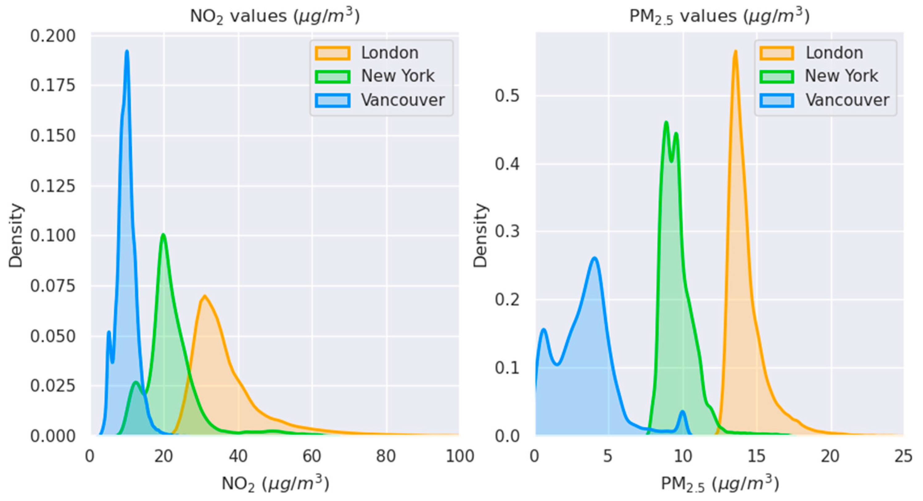
3.1. Intracity Performance for London, Vancouver, and New York

Separate labelled images for NO₂ and PM_2.5 were prepared for each of the three cities. Each of these images were matched with labels available from city-wide pollution rasters using the coordinate information for each image. We trained separate models for each city using four-fold cross validation. In each fold, 75% of the data (randomly selected image outcome pairs for 75% of grid points) were used for training the network and the remaining 25% were withheld. We then measured how well the trained network used images to estimate outcomes at locations that were not used in training from the same city. We repeated this process four times, holding out a different 25% of data each time.

Full results are available in Table 1. For NO₂, intracity models achieved r values of 0.79, 0.87, and 0.73 (R² = 0.58, 0.75, and 0.52) for London, New York, and Vancouver, respectively. Lower performances were observed for PM_2.5 where r values were 0.79, 0.85, and 0.60 (R² = 0.59, 0.71, 0.33). This was expected and consistent with previous work, as local variation for NO₂ is higher and influenced more by local (mobile) sources compared with PM_2.5, which is influenced by regional levels and secondary production. This is unlikely to be closely related to micro-scale spatial patterns of sources. Average RMSE values across cities were 4.3 µg/m³ for NO₂ and 1.0 µg/m³ for PM_2.5. The best performances were achieved in New York and the poorest performance was observed in Vancouver, particularly in areas of low pollution.

Figure 2 shows that the spatial patterns of pollution are better captured for NO₂ compared to PM_2.5 by image-based deep learning models. Similar patterns over space are observed for both label and prediction maps, even though predictions are only based on street-level images, i.e., no spatial information or smoothing method was used for generating prediction maps. Image-based deep learning models identify major roads and distinguish them from smaller streets. They also associate them with higher levels of pollution concentration. City centers characterized by higher building and population density are also identified and predicted as high-pollution areas. These results are consistent with inputs into LUR and dispersion models used as labels described in Section 2. Prediction errors for all cities were particularly high for low pollution areas. Spatial patterns in errors reflect the impact of features such as geography (e.g., proximity to the coast and mountains in Vancouver). This may, in part, reflect that street-level images are predominantly collected from streets by driving cars and therefore availability is limited for low pollution areas such as parks, forests, and coastal areas. The models use images only for predictions, with no additional information on the spatial context (such as proximity to parks, mountains, and oceans). Data from other sources (e.g., satellite images and built environment datasets) can be used to provide information about the spatial context within a multi-model learning framework and can help to improve performances in the future [20].

We used class activation maps (CAMs) for additional insights into image regions that are used by the model for making pollution predictions [37,42]. CAMs offer a post hoc visualization method using the average pooling layer at the end of ResNet18. Figure 3 shows some examples from locations where both the label and predicted pollution values were very high from each city. The areas of the image that substantially contribute positively to the final prediction value are highlighted in red. We observe that roads, cars, and high building density are being highlighted in these images. Interpretation of CAM visualizations become harder and less appealing for areas with mid- or low-range pollution levels (see more examples in Supplementary Materials). This could be related to the general difficulty of interpretability of deep learning models and associated inadequacies in the proposed CAM method, but could also potentially be explained by the fact that no specific image region is identified as a major source of pollution, which also correctly results in lower pollution estimates.

We analyzed the association between the model estimate results and ground monitoring site measurements separately for each study city. Sites that had co-located model estimates within a distance of less than 50 m were included. It was not possible to compute r for PM_2.5 in Vancouver as we only had two qualifying measurement sites. Correlations between estimated values and annual mean concentrations were high: NO₂ models achieved r values of 0.90, 0.76, and 0.97 (R² = 0.81, 0.58, 0.95, N = 8, 47, 4) for London, New York, and Vancouver, respectively. PM_2.5 models achieved r values of 0.72 for London and 0.86 for New York (R² = 0.51, 0.74, N = 9, 4). The number of available monitoring stations for evaluations were limited, so results should be interpreted with caution. These values are comparable to performances of the underlying model outputs used for training, suggesting that images can capture a substantial part of pollution sources often used as inputs for model training. We were unable to generate daily or hourly estimates of pollution as we were restricted by image availability.

3.2. Intracity Performance for London, Vancouver, and New York

For evaluating transferability of learning, we trained three separate models using three-fold cross validation. In each fold, combined data from two cities were used for training the network and the third city was withheld. We then measured how well the trained network used images to predict outcomes in the holdout city not used for training. Resultant performance metrics can be compared with the intracity results presented in the previous section. In regression tasks, it is well known that deep learning models do not generalize well previously unseen values. This was, by design, a specifically challenging setting, as label data distributions used for the selected three cities were almost non-overlapping for NO₂ and PM_2.5 (Figure 1). For example, when training with combined NO₂ data from Vancouver and New York, labels used in training were mostly ranged between 0 and 40 µg/m³. Accordingly, predictions were also in this range when making predictions in London. Yet, target data NO₂ concentrations were much higher in London, mostly ranging between 20 and 60 µg/m³ resulting in large RMSEs. As a result, estimation of absolute levels was poor. We also aimed to understand if it was possible to shift estimation distributions to match the target distributions, to achieve lower levels of absolute error. Furthermore, we sought to clarify whether our models were successful in capturing spatial variation and relative pollutant levels. For this purpose, we transformed and adjusted estimation distributions using the mean and standard deviation of the labels ($\overline{x}$ and ${\sigma }_x$) from the target city, using the following equation: $y\prime =\overline{x}+\left(y-\overline{y}\right)\ast \left({\sigma }_x/{\sigma }_y\right)$ where $y\prime$ and $y$ are the adjusted and pre-adjusted estimation values, respectively. This post hoc adjustment step influences RMSE and NRMSE values, but not r and R² values. In practice, some prior information on means and variation of air pollution levels from the target city will be required for this post hoc adjustment step. We reported performances from the adjusted model estimates in Table 1 and Figure 2 (results from non-adjusted model estimates are provided in the Supplementary Materials).

When the network trained on two source cities was used to make predictions in the hold out target city, the performances were much lower. The Pearson correlations between true (label) and predicted values were 0.42, 0.60, and 0.28 (R² = 0.18, 0.36, 0.08) in London, New York, and Vancouver for NO₂, and 0.37, 0.47, and 0.06 for PM_2.5 (R² = 0.14, 0.22, 0). These correlations were lower, and the errors were larger, than those for intracity results (Section 2.1). Correlations between estimated values and annual mean concentrations from ground monitoring stations were also lower, with r values ranging between 0.51 (R² = 0.00, N = 4) for Vancouver and New York (R² = 0.26, N = 47) and 0.82 (R² = 0.67, N = 8) in London for NO₂, and 0.29 (R² = 0.09, N = 4) in New York and 0.46 (R² = 0.22, N = 9) in London for PM_2.5. This is consistent with previous work where transferability of LUR models was evaluated [39,40,41], which found low performances of NO₂. Specifically, previous work reported that transferability performances of an LUR model trained on Vancouver was R² = 0.51 (N = 40) for Victoria (another city in Canada) and R² = 0.33 (N = 26) for Seattle (a city in another country). We observed similar performances from intercity NO₂ models: R² = 0.67 (N = 8) for London, R² = 0.26 (N = 47) for New York, and R² = 0.00 (N = 4) for Vancouver. We used less data input, yet our evaluation set was limited as we had limited numbers of available monitoring stations in London and Vancouver. Figure 2 shows that spatial variation for NO₂ can be captured to a limited degree. It is, however, much harder to transfer across cities to estimate spatial variability of PM_2.5. This likely results from differences in both important PM_2.5 sources between cities and regional influences on PM_2.5 spatial patterns (e.g., topographic and geographic), and from meteorological impacts on dispersion and secondary PM_2.5 production. For example, Vancouver is mountainous with sea breeze influences, which will not be identified by street-level images, while New York City is downwind of industrial emission sources and power generation facilities which were located outside of the imagery domain. Even though it is possible to transfer image-based deep learning models between cities, success will depend not only on visual similarity of features associated with pollution levels, but also differences in absolute levels and distributions of pollution between source and target cities. Some of this information is available from global models [43]. Further research is needed to investigate the most efficient approach to local calibration to help produce models that are as predictive as their performances in training cities [15,41].

Finally, we aimed to understand whether image-based estimates perform better in locations where local LUR and dispersion models have lower error. For a comparative analysis of image-based prediction errors and locally calibrated models (originally used as labels in training), we computed relative errors for each ground monitoring station location. The number of monitoring stations available for evaluation was unfortunately too low to generalize our findings. Still, as expected, intracity image-based errors for NO₂ were highly correlated with local LUR and dispersion model errors, with correlations of r = 0.62 (N = 8), 0.72 (N = 47), and 0.99 (N = 4) for London, New York, and Vancouver, respectively. When transferring between cities for NO₂, we got a much lower correlation for New York at 0.08 where we had the largest number of data points with N = 47. In other cities, the correlations remained relatively high at r = 0.60 for London, and r = 0.98 for Vancouver. For PM_2.5, within-city correlations between relative errors from intracity image-based estimates were r = 0.51 for London (N = 9) and r = 0.21 for New York (N = 4); we could not include Vancouver with N = 2. Intercity image-based transfer was even more difficult for PM_2.5, in line with other findings, where the correlations were very low or in the wrong direction, with r = 0.35 and r = −0.77. These findings are in line with our main results, where we showed that image-based models can learn local features when trained on image-label pairs from the same city. It is, however, much harder to transfer across cities.

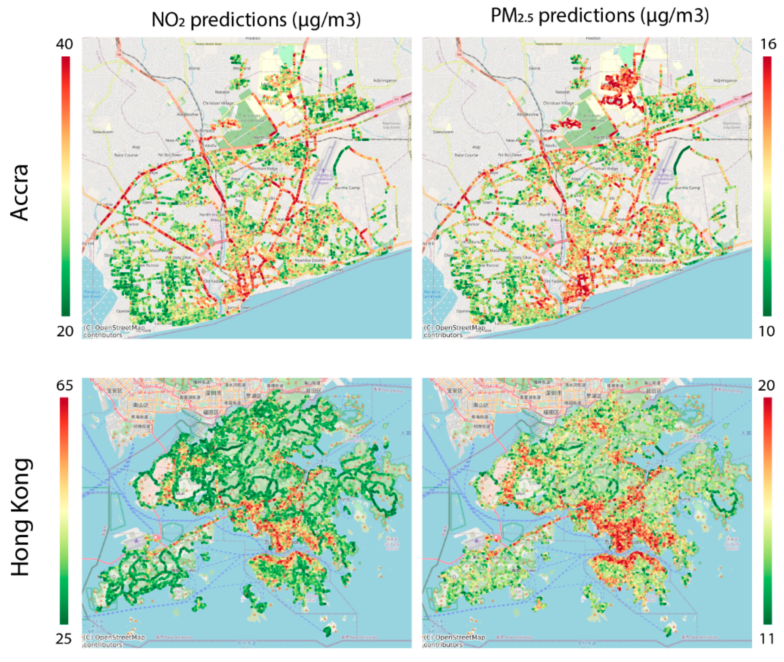
3.3. Evaluation of Transferability to Accra and Hong Kong

We evaluated how well a model trained on combined (pooled) data from all three source cities (London, New York, and Vancouver) performed in estimating pollution levels in Accra and Hong Kong. Evaluation of transferability performance is difficult for cities where city-wide estimates of annual pollutant levels are scarce. We used monitoring station data from field campaigns carried out for Hong Kong [33] and for Accra [18]. In Hong Kong, measurements were collected in two sampling campaigns during the warm and cool seasons. Roadside measurements of NO₂ were made for two- to three-week periods with Ogawa passive samplers at 97 locations. PM_2.5 was measured using TSI SidePak personal aerosol monitors at 84 sites for 24 h. Both NO₂ and PM_2.5 measurements at the above sites were adjusted for day-to-day variation, with continuous measurements made at a subset of four monitoring sites. A similar protocol was employed in Accra (10 year-long sites and 136 week-long sites). Sites with street-level images available within a 50m distance threshold were included for evaluations in Table 1.

Estimation maps shown in Figure 4 associate major roads and city centers with high pollution. However, when we evaluated performances with ground monitoring stations, the performances were poor (r = 0.46, R² = 0.21 (Hong Kong) and 0.21, R² = 0.06 (Accra) for NO₂, and r = 0.02, R² = 0.02 (Hong Kong) and 0.12, R² = 0.01 (Accra) for PM_2.5). In Hong Kong, higher pollution levels near China are not captured, as the images do not contain information on proximity to high pollution regions. The city center, however, is successfully identified as a relatively high pollution area.

4. Conclusions

The focus of this work was to understand whether and to what extent information contained in street-level images, with limited or no information on the local conditions, can predict spatial variation in annual pollution levels. Performance of image-based models when trained and tested on the same city for estimating mean annual levels of air pollution were high. Model performances of these deep learning models, using only images as input, were comparable to performances of traditional models that require substantially higher levels of input data. This suggests that images can capture a substantial part of pollution sources often used as inputs for model training, along with additional insights from post hoc visualizations highlighting image regions that are used by these models.

Similar to LUR models, transferability of models between cities in different geographies is difficult. Specifically, we found that transferability between Hong Kong and Accra was much more difficult than transferability between London, Vancouver, and New York. Image-based estimation models work better when transferring between cities that share similar sources of pollution. It is, however, a much larger challenge to transfer models calibrated in cities with fundamentally different sources of pollution (e.g., type of cars and biomass burning [44]). In other words, model ability is dependent on the similarity of underlying sources of pollution that can be captured by images only. Hence, their ability to scale up to global coverage is also dependent on availability of label data from cities with similar source profiles.

Our findings provide several open questions for future work. Would locally calibrated LUR model outputs for a city like Accra, where and when available, transfer well to other West African cities (e.g., Nigeria) with similar sources of pollution? Would image-based models transfer well to cities within the same country and over time? Can active learning approaches of machine learning be utilized for effective local calibration where the measurement points in target cities are sampled in an optimal way? Can images be combined with other globally available local sources of information (e.g., satellite-based air quality estimates, or aerial image satellite data on proximity to parks, oceans, and roads, or OpenStreetMaps) to make better predictions for scaling up globally? How can we modify data collection protocols to better utilize images and image-based predictions? Can daily or hourly estimates be generated if images are available at high temporal resolution? We hope that future research, based on this study, can address these questions and enable better models of pollutant levels with global coverage, to support global efforts to reduce pollutant levels and establish health effects.

References

1. Landrigan, P.J.; Fuller, R.; Acosta, N.J.R.; Adeyi, O.; Arnold, R.; Basu, N.; Baldé, A.B.; Bertollini, R.; Bose-O’Reilly, S.; Boufford, J.I.; et al. The Lancet Commission on pollution and health. Lancet 2018, 391, 462–512. [Google Scholar] [CrossRef] [Green Version]
2. Cohen, A.J.; Brauer, M.; Burnett, R.; Anderson, H.R.; Frostad, J.; Estep, K.; Balakrishnan, K.; Brunekreef, B.; Dandona, L.; Dandona, R.; et al. Estimates and 25-year trends of the global burden of disease attributable to ambient air pollution: An analysis of data from the Global Burden of Diseases Study 2015. Lancet 2017, 389, 1907–1918. [Google Scholar] [CrossRef] [Green Version]
3. Hoek, G.; Krishnan, R.M.; Beelen, R.; Peters, A.; Ostro, B.; Brunekreef, B.; Kaufman, J.D. Long-term air pollution exposure and cardio-respiratory mortality: A review. Environ. Health 2013, 12, 43. [Google Scholar] [CrossRef] [Green Version]
4. Schraufnagel, D.E.; Balmes, J.R.; Cowl, C.T.; De Matteis, S.; Jung, S.-H.; Mortimer, K.; Perez-Padilla, R.; Rice, M.B.; Riojas-Rodriguez, H.; Sood, A.; et al. Air Pollution and Noncommunicable Diseases: A Review by the Forum of International Respiratory Societies’ Environmental Committee, Part 1: The Damaging Effects of Air Pollution. Chest 2019, 155, 409–416. [Google Scholar] [CrossRef] [PubMed] [Green Version]
5. Brauer, M.; Amann, M.; Burnett, R.T.; Cohen, A.; Dentener, F.; Ezzati, M.; Henderson, S.B.; Krzyzanowski, M.; Martin, R.V.; Van Dingenen, R.; et al. Exposure assessment for estimation of the global burden of disease attributable to outdoor air pollution. Environ. Sci. Technol. 2012, 46, 652–660. [Google Scholar] [CrossRef] [PubMed] [Green Version]
6. Ryan, P.H.; Lemasters, G.K. A review of land-use regression models for characterizing intraurban air pollution exposure. Inhal. Toxicol. 2007, 19 (Suppl. 1), 127–133. [Google Scholar] [CrossRef] [Green Version]
7. Martin, R.V.; Brauer, M.; van Donkelaar, A.; Shaddick, G.; Narain, U.; Dey, S. No one knows which city has the highest concentration of fine particulate matter. Atmos. Environ. 2019, 3, 100040. [Google Scholar] [CrossRef]
8. Weichenthal, S.; Hatzopoulou, M.; Brauer, M. A picture tells a thousand… exposures: Opportunities and challenges of deep learning image analyses in exposure science and environmental epidemiology. Environ. Int. 2019, 122, 3–10. [Google Scholar] [CrossRef]
9. Apte, J.S.; Messier, K.P.; Gani, S.; Brauer, M.; Kirchstetter, T.W.; Lunden, M.M.; Marshall, J.D.; Portier, C.; Vermeulen, R.C.; Hamburg, S.P. High-Resolution Air Pollution Mapping with Google Street View Cars: Exploiting Big Data. Environ. Sci. Technol. 2017, 51, 6999–7008. [Google Scholar] [CrossRef]
10. Messier, K.P.; Chambliss, S.E.; Gani, S.; Alvarez, R.; Brauer, M.; Choi, J.J.; Hamburg, S.P.; Kerckhoffs, J.; LaFranchi, B.; Lunden, M.M.; et al. Mapping air pollution with google street view cars: Efficient Approaches with mobile monitoring and land use regression. Environ. Sci. Technol. 2018, 52, 12563–12572. [Google Scholar] [CrossRef] [Green Version]
11. Hong, K.; Weichenthal, S. A New Method of Estimating Global PM2. 5 Concentrations using Satellite Images. Environ. Epidemiol. 2019, 3, 432. [Google Scholar]
12. Ganji, A.; Minet, L.; Weichenthal, S.; Hatzopoulou, M. Predicting Traffic-Related Air Pollution Using Feature Extraction from Built Environment Images. Environ. Sci. Technol. 2020, 54, 10688–10699. [Google Scholar] [CrossRef] [PubMed]
13. Hong, K.Y.; Pinheiro, P.O.; Weichenthal, S. Predicting outdoor ultrafine particle number concentrations, particle size, and noise using street-level images and audio data. Environ. Int. 2020, 144, 106044. [Google Scholar] [CrossRef] [PubMed]
14. Sorek-Hamer, M.; Just, A.C.; Kloog, I. The Use of Satellite Remote Sensing in Epidemiological Studies. Curr. Opin. Pediatr. 2016, 28, 228. [Google Scholar] [CrossRef] [Green Version]
15. Suel, E.; Polak, J.W.; Bennett, J.E.; Ezzati, M. Measuring social, environmental and health inequalities using deep learning and street imagery. Sci. Rep. 2019, 9, 1–10. [Google Scholar] [CrossRef]
16. Qi, M.; Hankey, S. Using Street View Imagery to Predict Street-Level Particulate Air Pollution. Environ. Sci. Technol. 2021, 55, 2695–2704. [Google Scholar] [CrossRef]
17. Hoek, G.; Beelen, R.; de Hoogh, K.; Vienneau, D.; Gulliver, J.; Fischer, P.; Briggs, D. A review of land-use regression models to assess spatial variation of outdoor air pollution. Atmos. Environ. 2008, 42, 7561–7578. [Google Scholar] [CrossRef]
18. Clark, S.N.; Alli, A.S.; Brauer, M.; Ezzati, M.; Baumgartner, J.; Toledano, M.B.; Hughes, A.F.; Nimo, J.; Moses, J.B.; Terkpertey, S.; et al. High-resolution spatiotemporal measurement of air and environmental noise pollution in Sub-Saharan African cities: Pathways to Equitable Health Cities Study protocol for Accra, Ghana. BMJ Open 2020, 10, 35798. [Google Scholar] [CrossRef]
19. LeCun, Y.; Bengio, Y.; Hinton, G. Deep learning. Nature 2015, 521, 436–444. [Google Scholar] [CrossRef]
20. Suel, E.; Bhatt, S.; Brauer, M.; Flaxman, S.; Ezzati, M. Multimodal deep learning from satellite and street-level imagery for measuring income, overcrowding, and environmental deprivation in urban areas. Remote Sens. Environ. 2021, 257, 112339. [Google Scholar] [CrossRef]
21. de Hoogh, K.; Gulliver, J.; van Donkelaar, A.; Martin, R.V.; Marshall, J.D.; Bechle, M.J.; Cesaroni, G.; Pradas, M.C.; Dedele, A.; Eeftens, M.; et al. Development of West-European PM2. 5 and NO2 land use regression models incorporating satellite-derived and chemical transport modelling data. Environ. Res. 2016, 151, 1–10. [Google Scholar] [CrossRef] [PubMed] [Green Version]
22. Beelen, R.; Hoek, G.; Vienneau, D.; Eeftens, M.; Dimakopoulou, K.; Pedeli, X.; Tsai, M.-Y.; Künzli, N.; Schikowski, T.; Marcon, A.; et al. Development of NO2 and NOx land use regression models for estimating air pollution exposure in 36 study areas in Europe—The ESCAPE project. Atmos. Environ. 2013, 72, 10–23. [Google Scholar] [CrossRef]
23. City of New York. The New York City Community Air Survey: Neighborhood Air Quality 2008–2014. 2017. Available online: https://www1.nyc.gov/site/doh/data/data-sets/air-quality-nyc-community-air-survey.page (accessed on 14 July 2022).
24. Henderson, S.B.; Beckerman, B.; Jerrett, M.; Brauer, M. Application of land use regression to estimate long-term concentrations of traffic-related nitrogen oxides and fine particulate matter. Environ. Sci. Technol. 2007, 41, 2422–2428. [Google Scholar] [CrossRef] [PubMed]
25. Bechle, M.J.; Millet, D.B.; Marshall, J.D. National spatiotemporal exposure surface for NO2: Monthly scaling of a satellite-derived land-use regression, 2000—2010. Environ. Sci. Technol. 2015, 49, 12297–12305. [Google Scholar] [CrossRef]
26. Smith, R.B.; Fecht, D.; Gulliver, J.; Beevers, S.D.; Dajnak, D.; Blangiardo, M.; Ghosh, R.E.; Hansell, A.L.; Kelly, F.J.; Anderson, H.R.; et al. Impact of London’s road traffic air and noise pollution on birth weight: Retrospective population based cohort study. BMJ 2017, 359, 5299. [Google Scholar] [CrossRef] [Green Version]
27. Clean Air for London. London Atmospheric Emissions Inventory (LAEI) 2010. 2010. Available online: https://data.london.gov.uk/dataset/london-atmospheric-emissions-inventory-2010 (accessed on 14 July 2022).
28. Wang, R.; Henderson, S.B.; Sbihi, H.; Allen, R.W.; Brauer, M. Temporal stability of land use regression models for traffic-related air pollution. Atmos. Environ. 2013, 64, 312–319. [Google Scholar] [CrossRef]
29. U.S. EPA. US EPA Air Quality Download Data. 2020. Available online: https://aqs.epa.gov/aqsweb/airdata/download_files.html (accessed on 14 July 2022).
30. Government of Canada. Environment and Climate Change Canada Data. 2020. Available online: http://data.ec.gc.ca/data/?lang=en (accessed on 14 July 2022).
31. Imperial College. London Air Quality Network. 2020. Available online: https://www.londonair.org.uk/london/asp/reportdetail.asp?ReportID=lars2010 (accessed on 14 July 2022).
32. Lang, P.E.; Carslaw, D.C.; Moller, S.J. A trend analysis approach for air quality network data. Atmos. Environ. 2019, 2, 100030. [Google Scholar] [CrossRef]
33. Lee, M.; Brauer, M.; Wong, P.; Tang, R.; Tsui, T.H.; Choi, C.; Cheng, W.; Lai, P.-C.; Tian, L.; Thach, T.-Q.; et al. Land use regression modelling of air pollution in high density high rise cities: A case study in Hong Kong. Sci. Total Environ. 2017, 592, 306–315. [Google Scholar] [CrossRef] [Green Version]
34. Alli, A.S.; Clark, S.N.; Hughes, A.F.; Nimo, J.; Bedford-Moses, J.; Baah, S.; Wang, J.; Vallarino, J.; Agyemang, E.; Barratt, B.; et al. Spatial-temporal patterns of ambient fine particulate matter (PM2.5) and black carbon (BC) pollution in Accra. Environ. Res. Lett. 2021, 16, 074013. [Google Scholar] [CrossRef]
35. Wang, J.; Alli, A.S.; Clark, S.; Hughes, A.; Ezzati, M.; Beddows, A.; Vallarino, J.; Nimo, J.; Bedford-Moses, J.; Baah, S.; et al. Nitrogen oxides (NO and NO2) pollution in the Accra metropolis: Spatiotemporal patterns and the role of meteorology. Sci. Total Environ. 2022, 803, 149931. [Google Scholar] [CrossRef]
36. He, K.; Zhang, X.; Ren, S.; Sun, J. Deep residual learning for image recognition. In Proceedings of the IEEE Conference on Computer Vision and Pattern Recognition, Las Vegas, NV, USA, 27–30 June 2016; pp. 770–778. [Google Scholar]
37. Zhou, B.; Khosla, A.; Lapedriza, A.; Oliva, A.; Torralba, A. Learning Deep Features for Discriminative Localization. In Proceedings of the IEEE Conference on Computer Vision and Pattern Recognition (CVPR), 2016. pp. 2921–2929. [CrossRef] [Green Version]
38. Torch Contributors. Torchvision Models. 2017. Available online: https://pytorch.org/vision/stable/models.html (accessed on 13 July 2022).
39. Briggs, D.J.; de Hoogh, C.; Gulliver, J.; Wills, J.; Elliott, P.; Kingham, S.; Smallbone, K. A regression-based method for mapping traffic-related air pollution: Application and testing in four contrasting urban environments. Sci. Total Environ. 2000, 253, 151–167. [Google Scholar] [CrossRef]
40. Jerrett, M.; Arain, A.; Kanaroglou, P.; Beckerman, B.; Potoglou, D.; Sahsuvaroglu, T.; Morrison, J.; Giovis, C. A review and evaluation of intraurban air pollution exposure models. J. Expo. Anal. Environ. Epidemiol. 2005, 15, 185–204. [Google Scholar] [CrossRef] [PubMed]
41. Poplawski, K.; Gould, T.; Setton, E.; Allen, R.; Su, J.; Larson, T.; Henderson, S.; Brauer, M.; Hystad, P.; Lightowlers, C.; et al. Intercity transferability of land use regression models for estimating ambient concentrations of nitrogen dioxide. J. Expo. Sci. Environ. Epidemiol. 2009, 19, 107–117. [Google Scholar] [CrossRef] [PubMed] [Green Version]
42. Simonyan, K.; Vedaldi, A.; Zisserman, A. Deep Inside Convolutional Networks: Visualising Image Classification Models and Saliency Maps. 2013. Available online: http://arxiv.org/abs/1312.6034 (accessed on 14 October 2017).
43. McDuffie, E.E.; Martin, R.V.; Spadaro, J.V.; Burnett, R.; Smith, S.J.; O’Rourke, P.; Hammer, M.S.; van Donkelaar, A.; Bindle, L.; Shah, V.; et al. Source sector and fuel contributions to ambient PM2.5 and attributable mortality across multiple spatial scales. Nat. Commun. 2021, 12, 1–12. [Google Scholar] [CrossRef]
44. Dionisio, K.; Arku, R.; Hughes, A.; Vallarino, J. Air Pollution in Accra Neighborhoods: Spatial, Socioeconomic, and Temporal Patterns. Environ. Sci. Technol. 2010, 44, 2270–2276. [Google Scholar] [CrossRef]
Figure 1. Distributions of annual mean estimates of NO2 and PM2.5 from local land use regression and dispersion models. Figures show a clear distinction of air pollutant levels between the 3 study cities. These values are used as labels when training deep learning models using street-level images.
Remotesensing 14 03429 g001
Figure 2. Comparison of labels and prediction maps of mean NO2 and PM2.5 levels for London, New York, and Vancouver. The label column displays the base map and the extent of the shapefiles used. We adjusted the color bar scale to visualize the spatial patterns for each city and pollutant, where red areas correspond to high pollution and green to low pollution. Intracity model predictions show results from experiments where networks were trained and tested on images from the same city using 4-fold cross validation. Intercity model predictions show results from experiments where the models were trained on combined data from two cities and tested on the third held-out city. Relative errors (absolute error divided by the magnitude of the label value) are also displayed where darker red colors indicate higher error rates.
Remotesensing 14 03429 g002
Figure 3. Examples of class activation maps from (A) London, (B) New York, and (C) Vancouver. These examples were selected from locations where both the label and prediction NO2 values were high, as follows: 53.3 µg/m3 and 76 µg/m3 for (A), 20.8 µg/m3 and 16.7 µg/m3 for (B), and 63.5 µg/m3 and 61.3 µg/m3 for (C). Red areas indicate parts of the image that the network considers as positively influencing pollution levels. The visualizations show that the network identifies cars, roads, and high-density buildings as major sources of pollution. More examples are available in the Supplementary Materials that are less appealing and harder to interpret, especially from areas with low- and mid-range pollution levels.
Remotesensing 14 03429 g003
Figure 4. Prediction maps of mean NO2 and PM2.5 levels for Accra and Hong Kong. Models were trained on combined data from London, New York, and Vancouver and tested on images for Accra and Hong Kong. We adjusted the color bar scale to visualize the spatial patterns for each city and pollutant, where red areas correspond to high pollution and green to low pollution.
Remotesensing 14 03429 g004