Abstract
Leaf-level hyperspectral-based species identification has a long research history. However, unlike hyperspectral image-based species classification models, convolutional neural network (CNN) models are rarely used for the one-dimensional (1D) structured leaf-level spectrum. Our research focuses on hyperspectral data from five laboratories worldwide to test the general use of effective identification of the CNN model by reshaping 1D structure hyperspectral data into two-dimensional greyscale images without principal component analysis (PCA) or downscaling. We compared the performance of two-dimensional CNNs with the deep cross neural network (DCN), support vector machine, random forest, gradient boosting machine, and decision tree in individual tree species classification from leaf-level hyperspectral data. We tested the general performance of the models by simulating an application phase using data from different labs or years as the unseen data for prediction. The best-performing CNN model had validation accuracy of 98.6%, prediction accuracy of 91.6%, and precision of 74.9%, compared to the support vector machine, with 98.6%, 88.8%, and 66.4%, respectively, and DCN, with 94.0%, 85.7%, and 57.1%, respectively. Compared with the reference models, CNNs more efficiently recognized Fagus crenata, and had high accuracy in Quercus rubra identification. Our results provide a template for a species classification method based on hyperspectral data and point to a new way of reshaping 1D data into a two-dimensional image, as the key to better species prediction. This method may also be helpful for foliar trait estimation.
1. Introduction
Plant species discrimination is essential because of concerns about climate change and the resultant changes in geographic distribution and species abundance. However, identifying plants by conventional keys is complex and time-consuming, and the use of specific botanical terms is frustrating to non-experts [1]. The development of digital cameras and computer vision-related techniques significantly boosts automated image-based species identification [2,3,4], which extracts features based on leaf shape, texture, color, or venation [2]. Designing and orchestrating such methods are problem-specific, with models customized to specific applications [4]. Deep artificial neural networks (ANNs) such as the convolutional neural network (CNN) automate the critical feature-extraction step by learning a suitable representation of the training data and systematically developing a robust classification model, producing promising and constantly improving results in automated plant species classification [4]. Furthermore, identification utilizing CNNs reached an average accuracy of 99.5% on the ILSVRC2012 dataset covering 44 species [5,6], and a 26-layer network ResNet architecture achieved 99.65% accuracy on the Flavia dataset [7]. Nevertheless, more general image processing issues, such as ambiguity caused by unknown illumination and poses remain problematic [3], and image-based species identification consumes many storage, network, and computational resources. Although leaf hyperspectral data are more difficult to obtain than image data, (1) their acquisition uses a standard process, with no image processing problems such as illumination angle and positions; (2) the structured data are small; and (3) they require fewer computer resources.
Several machine learning methods have been commonly applied for species discrimination based on hyperspectral data, such as linear discriminant analysis (LDA), maximum likelihood (ML), spectral angle mapper (SAM), logistic regression (LR), gradient boosting machine (GBM), random forest (RF), and support vector machine (SVM) [8,9,10,11]. For instance, an overall accuracy of 86% was achieved with an object-based LDA classifier for better discrimination of seven species of emergent trees in a lowland tropical rain forest based on spectrometer and airborne hyperspectral reflectance data [10], while an SVM study on major forests and plant species discrimination in the Mudumalai forest region in India showed a very high accuracy of 92.37% [12]. A study in a Jamaican tropical wetland obtained 91.8% and 84.8% accuracy with importance-ranked spectral indices and reflectance spectra, respectively, using an RF classifier to discriminate 46 plant species [13]. More recent research using LR to discriminate 26 tropical dry forest tree species had an overall accuracy of 89% [14]. These results have demonstrated the good performance and large potential of machine learning in plant species identification.
Deep learning methods such as ANNs and CNNs have also been used. Gong et al. [15] suggested the performance of ANN was better than that of LDA, obtaining an accuracy of 91% when using only average sunlit samples for the identification of six conifer tree species. Similarly, the application of a CNN classifier to high-resolution hyperspectral and RGB imagery labeled to predict tree species at a pixel level was solid at species-level classification in a Sierran mixed-conifer forest [16]. A 3D-CNN utilizing 4 m airborne hyperspectral image patches achieved an overall F1-score (harmonic mean of recall and precision) of 0.86 and accuracy of 87% when classifying Scots pine, Norway spruce, and birch, and could more efficiently distinguish coniferous species than other models [17]. Furthermore, a 3D-1D-CNN model could reduce computation while achieving 93.14% accuracy when classifying eight species based on airborne hyperspectral remote sensing data [18].
Classification with hyperspectral measurements, acquired by narrowband spectroradiometers or imaging sensors, generally required some form of spectral feature selection to reduce the dimensionality of the data to a level suitable for the construction of a classification model [19]. Bands selected using an ensemble of methods improved logistic regression classification performance by 3% compared to a result without band selection [14]. Optimal regions of the spectrum for species discrimination varied with scale. However, near-infrared (700–1327 nm) bands were consistently important regions across all scales [10,19,20]. Bands in the visible (437–700 nm) and shortwave infrared (1994–2435 nm) regions were more critical at pixel and canopy scales [10]. However, the possibility of discriminatory spectral regions being associated with specific taxonomic, structural, or functional groupings of plants is inconclusive due to variability between studies [19]. Moreover, spectral feature selection mainly suits classification models, as the full wavelength is too complicated. However, such preprocessing can be ignored when using the CNN model. CNNs outperform standard chemometric methods, especially for classification tasks with no preprocessing [21], for images made of 10,000 pixels (values) with associated color information, obtaining very high accuracy in recognition problems [17]. Moreover, CNNs can effectively extract spatial information and share weights by establishing local connections, which greatly reduces model parameters and provides a way to extract features from the original input image [22]. As a result, CNN models are commonly used for species discrimination based on hyperspectral image data.
Continuous efforts have been made to construct a practical plant species classification model based on hyperspectral data [15,19,23]. Leaf spectroscopy data are related to carotenoid/chlorophyll, carbon, water, and leaf mass per area [24,25,26], which are on the biochemical level, whereas leaf image data are on an organic level. Moreover, broad plant groups, orders, and families, and can be identified from reflectance spectra due to the phylogenetic signals present in leaf spectra [27]. Hence these kinds of datasets are ideal for species discrimination. Unfortunately, few studies have applied CNN models based on leaf spectroscopy data, which are in general 1D structured data, while CNNs are mostly used for multidimensional image data. However, reshaping 1D leaf spectral data into a two-dimensional (2D) matrix may provide a solution. Since leaf-level hyperspectral data are taken as multidimensional in most studies, PCA or downscaling is essential for modeling. In comparison, few studies ever consider reshaping these data to find more information, although this is a common task in practical data analysis [28,29,30,31]. Luo et al. [32] extracted a 1D spectral-spatial feature from a hyperspectral image target pixel and its neighbors, then stacked it into a 2D matrix to feed a CNN, and found that the performance of hyperspectral image classification had improved. Han and Gao [33] found that a reshaped image established by a pixel-level spectral was good enough to detect aflatoxin in peanuts, with a recognition rate above 95%.
In this study, we demonstrate the effective identification of plant species with a CNN model fed by a reshaped 2D greyscale image input from 1D hyperspectral data without PCA or downscaling. This is based on composite data including six tree species from different locations: Acer pseudoplatanus L., Acer rubrum L., Acer shirasawanum Koidzumi, Andropogon gerardii Vitman, Fagus crenata Blume, and Quercus rubra L. The constructed CNN model is compared extensively with deep cross neural network (DCN), SVM, RF, GBM, and DT models. To our knowledge, no previous attempt has been made to rearrange leaf spectroscopy data to a higher dimension for species identification modeling.
2. Materials and Methods
2.1. Dataset Description
2.1.1. Data Source
The measured database is a compilation of five independent datasets: ANGERS (AN), LOPEX93 (LO), NEON (NE, Fresh Leaf Spectra to Estimate LMA over NEON domains in the eastern United States Dataset, University of Wisconsin Environmental Spectroscopy Laboratory) [34], CCLTER (CC, FAB Leaf Spectra Across a Light Gradient at Cedar Creek LTER, Cavender-Bares Lab, College of Biological Sciences, University of Minnesota, Saint Paul) [35], and SHIZUOKA (SH, Shizuoka University). Figure 1 shows the worldwide distribution of data sources.
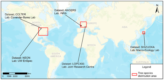
Figure 1.
Data source and tree species distribution: ANGERS; LOPEX93; NEON; CCLTER; SHIZUOKA.
The reflectance spectra of AN, NE, and SH were measured using an ASD Field Spec, of CC using a Spectral Evolution PSR+, and of LO using a Perkin–Elmer Lambda 19 spectroradiometer. Respective samples in the AN, LO, and NE datasets had 2, 5, and 5 or 10 replicates. Some species in the AN, LO, NE, and SH datasets were sampled more than once to incorporate variability due to the development stage. The CC dataset had only one measurement per leaf, each an automatic average of multiple spectra. The reflectance spectra of AN, NE, SH, and LO were measured at 1 nm resolution, and the software automatically resampled CC to 1 nm resolution and interpolated over sensor overlap. Datasets were measured between 350 (400) and 2450 (2500) nm, except CC (Andropogon gerardii Vitman), which was measured between 400 and 2400 nm. As we mainly used wavelengths between 400 and 2450 nm, those outside that range were removed; for CC (A. gerardii), the 2400 nm value was used to fill the range from 2401 to 2450.
2.1.2. Plant Species Selection
Training a classification model with thousands of spectral features generally requires a large sample size. However, since the collection of samples for hyperspectral studies is onerous, with high costs for imagery and arduous field measurements, sample sizes tend to be small [19]. A deep learning model needs enough samples for training and validation; BeamLab suggests 100–1000 samples [36]. In this study, species selection is based on sample sizes in the collected dataset and whether there are enough prediction items for each species. For datasets from one laboratory, it is hard to get enough hyperspectral data samples for each species. We chose a sample from more than 80 places and laboratories as the target species, and finally selected Acer pseudoplatanus L., Acer rubrum L., Acer shirasawanum Koidzumi, Andropogon gerardii Vitman, Fagus crenata Blume, and Quercus rubra L., and a total of 945 samples were included in this study. The sample size, symbol, and code for each species are shown in Table 1. The general performance of models was tested using data from different laboratories or years by separating them for training and prediction data, and the training leaf spectra are shown in Figure 2.

Table 1.
Source of training, validation, and prediction datasets (AN = ANGERS, NE = NEON, SH = SHIZUOKA, CC = CCLTER, LO = LOPEX).
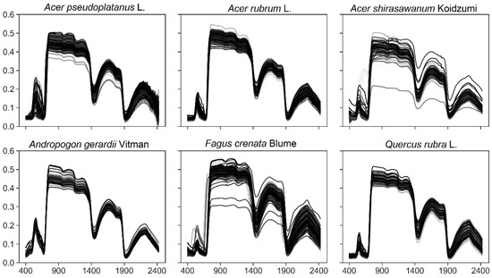
Figure 2.
Training and validation of leaf spectra of selected species.
2.1.3. Image Data Preparation for CNN Models
Unlike most conventional methods, we reshape 1D reflectance data into 2D grey image data as the input of the CNN model. To our knowledge, the reshaping of 1D leaf spectral data to 2D images as CNN training data has not been investigated. We use NumPy to reshape 1D leaf reflectance data into a 2D array, and Keras image preprocessing to save the array to a grey image, in the Python platform. The reflectance data was reshaped into a 45 × 45 square image. To get such a 2D image, we select wavelengths from 400 to 2424, which contain 2025 features, which we reshape into a 45 × 45 grey image, where each pixel represents a feature. During this process, leaf reflectance values from 0 to 1 are scaled from 0 to 255 (Figure 3).
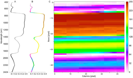
Figure 3.
Sample of one reflectance structure data item reshaped into a 45 × 45 shape image. (A): original reflectance structure data; (B): colorized reflectance structure data; (C): reshaped 2D image data. Reflectance wavelengths range from 400–2424 nm, and 2025 features are selected. Generated origin image is greyscaled, and the sample image is colorized to better understand each part of the reflectance. Reflectance values in the range 0–1 are reshaped into the grey image, with integer values scaled to 0–255. Hence, row 0 and column 0 represent 400 nm wavelength scaled value, and row −44 and column 44 represent 2424 nm.
2.2. CNN Model Architectures
Eight fully convolutional neural networks (CNNs) based on leaf reflectance data for species identification were developed. Each model contains one input layer, one or more convolution (Conv) and pooling (Pooling) layers, one flattened (Flatten) layer, one dense (Dense) layer, and one output layer with six channels (dense) corresponding to the six species. These models differ mainly by the number of Conv and Pooling layers. Table 2 summarizes the CNN model architecture. Figure 4 shows the CNN8 architecture in this study.
Table 2.
Summary of CNN model architecture. Numbers 1, 2, 3 after CNN indicate number of convolutional layers; A, B, C show difference of pooling layer after convolutional layers.
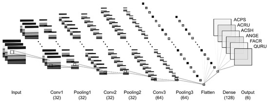
Figure 4.
CNN3C architecture: three convolutional layers (Conv1, Conv2, Conv3), pooling layer, flatten layer, fully connected dense layer, output layer, with six dense channels corresponding to the six species.
The input of the model is the reshaped 2D grey image. The grey image value in the [0, 255] range is rescaled to [0, 1] using the Keras preprocessing rescaling function, and this value is passed as the input of the first convolutional layer. Convolutional layers Conv1, Conv2 have 32 neurons, and Conv3 has 64 neurons, each with a 3 × 3 filter, and the stride is 1. Some models with a pooling layer use max pooling for 2D spatial data, with 2 × 2 default pooling sizes, with no stride and valid padding. Layer Flatten is used to concatenate the parallel outputs of the Conv or Pooling layer and convert them to a 1D vector, which is fed into the fully connected dense layer. The Flatten layer has no parameters to be trained. Instead, a dropout layer (rate of 0.2) before the flattening layer is adopted to prevent model overfitting and improve computing performance by randomly killing off many neurons [37]. We use the rectified linear unit (ReLU) activation function [38] for the convolutional layers and fully connected layer, and use the Adam optimizer [39] to train the model and find a local minimum of the objective function; sparse categorical cross-entropy is used to compute the cross-entropy loss between labels and predictions.
2.3. Model Comparison
The performance of eight CNN models is compared, and the best model is selected to compare with other typical models.
2.3.1. Comparison of CNN Models with DCN
The CNN models were compared to DCN, another artificial neural network that starts with an embedding and stacking layer, followed by a cross-network and deep network in parallel, and a final layer that combines their outputs [40]. Although traditional feedforward neural networks learn feature crosses inefficiently, DCN shows limited expressiveness in its cross-network at learning more predictive feature interactions [41] and has lower log loss than a deep neural network with fewer parameters by nearly an order of magnitude [40]. The same wavelength in CNN models was used in DCN to discriminate species without PCA analysis or downscaling. DCN architectures are the same as used by Wang et al. [40]. DCN codes are from Keras Code Examples [42]. An early stopping strategy is used to avoid overfitting.
2.3.2. Comparison of CNN Models with Conventional Models
To compare CNN models with other classification methods, four popular nonlinear or linear conventional classification approaches, namely SVM, RF, decision tree (DT), and gradient boosting decision tree (GBDT) were considered (Figure 5). Input data were structured leaf reflectance data standardized using the Sickie-learn preprocessing standard scaler. All models were implemented on the Anaconda Python platform using TensorFlow-Keras [43] and the Scikit-learn [44] library on a Windows 10 desktop with 32 GB RAM and an Nvidia Geforce GTX3070 graphics card with 12 GB RAM.
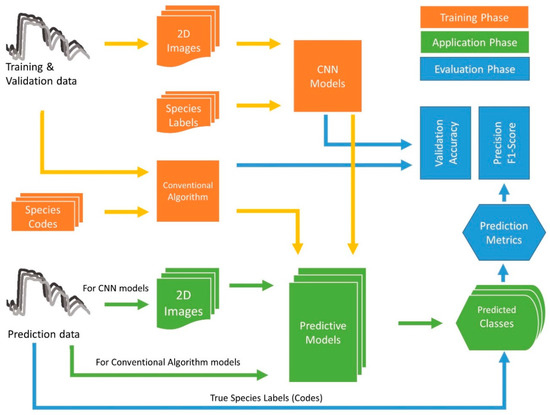
Figure 5.
Flowchart of the process followed in this study [4]. In the training phase, 1D structured reflectance data are reshaped into a 2D grey image as the input for CNN models, while 1D data are used for DCN and conventional algorithms. The application phase is a simulated phase using unseen data for trained model prediction. Unseen data are from different areas, labs, or years. Predicted and actual species are compared to generate prediction metrics.
SVM is a supervised nonparametric statistical learning technique [45]. SVMs are particularly appealing in remote sensing due to their ability to work with small training datasets, often with higher classification accuracy than traditional methods [46]. We compared linear, RBF, poly, and sigmoid kernels for SVM (Figure S1). The probability estimates of each class were calculated using five-fold cross-validation, and the linear kernel implemented a one-vs-the-rest multiclass strategy to train six classes.
The RF classifier is based on the classification tree approach and is efficient on large datasets with high accuracy [1]. We used 100 estimators, using gini as the criterion, with a max depth of 5.
DTs play an essential role in artificial intelligence and SVM applications [47]. They can easily interpret rules used to categorize datasets while simultaneously finding the relative importance of variables in the studied system [48]. We optimized DT with the gini criterion and best splitter, and expanded nodes until all leaves were pure.
GBDT is a family of powerful machine learning techniques that have shown success in a wide range of applications [49]. This accurate and effective off-the-shelf procedure can be used for regression and classification problems in areas including Web search ranking and ecology. The GBDT was optimized with a deviance loss function, 0.1 learning rate, 100 estimators, and maximum depth of 3.
2.4. Model Evaluation
In most species’ discrimination or classification studies, the test or validation matrix is used to evaluate model performance. However, this is limited to a dataset collected by one laboratory in one study field. Therefore, the evaluated model may not perform well for other reflectance datasets.
We collected datasets from different areas and laboratories and divided the experiment into training and simulated application phases. We used AN, NE, and SH data for training and validation, and LO, CC, and SH (different years) data for prediction in the application phase. We evaluated the general performance of the models by the prediction accuracy, precision, and F1-score, which can be obtained from a confusion matrix based on their phases [50]. A confusion matrix allows the visualization of the performance of an algorithm. Based on the actual and predicted labels of a species, data samples can be divided in four buckets, as shown in Table 3: true positive—actual = 1, predicted = 1; false positive—actual = 0, predicted = 1; false negative—actual = 1, predicted = 0; and true negative—actual = 0, predicted = 0.
Table 3.
Actual and predicted label confusion matrix.
Accuracy is the proportion of correctly identified positive and negative values,
Sensitivity (or recall) is the proportion of correctly predicted positive events,
Precision is the proportion of predicted positive events that are actually positive,
The F1-score is the harmonic mean of recall and precision, where a higher score indicates a better model, balancing precision (exactness) and sensitivity (completeness),
All models were trained and validated 100 times for a dataset, which was randomly divided into training and validation in a 75:25 ratio, and a final model was saved for the application phase to identify species in the prediction dataset. The actual and predicted species labels were used to calculate prediction metrics.
2.5. Process Flowchart
This study includes training and validation, simulate application, and evaluation phases. In the training phase (orange in Figure 5), training and validation data are reshaped to 2D images for CNN and taken directly as input for conventional algorithms. Validation accuracy is generated in this phase. Both CNN and conventional algorithms then generate predictive models. We take the prediction dataset as the unseen data for identification and simulate this phase (green in Figure 5) to evaluate the general performance of each model. The actual species labels and identified labels are used to calculate confusion metrics. Validation accuracy from the training phase, precision, and F1-score from the application phase are used to evaluate each model’s performance (blue in Figure 5). By adding the simulated application phase, we determine whether the predictive models can be widely used for leaf reflectance data from different places, labs, and periods.
3. Results
3.1. Comparison of CNN Models
All CNN models had high validation accuracy in the training phase. CNN1B, CNN2B, and CNN2C reached 98.6%, demonstrating high performance in species discrimination (Table 4). CNN2A had 98.0% accuracy, the lowest among these models.
Table 4.
Predictive results obtained by CNN models: mean and standard deviation of validation accuracy, prediction accuracy, precision, and F1-score from 100 runs.
In the application phase, the end-to-end learning approach of CNN2C obtained a mean prediction accuracy of 91.6%, precision of 74.9%, and F1-score of 0.65 (Table 4), which was much better than the other models. The second best performance was that of CNN3B, with a mean prediction accuracy of 91.2%, precision of 73.6%, and F1-score of 0.63. CNN1A and CNN2A obtained a mean prediction accuracy of 87.6%; precision of 62.9% and 62.7%, respectively; and F1-score of 0.54, which shows they could not discriminate the six species as well as other models in this phase.
3.2. Comparison of CNN with DCN and Conventional Models
DCN obtained a validation accuracy of 94.0% in the training phase (Table 5), 4.9% lower than CNN2C. In the application phase, DCN had a mean prediction accuracy of 85.5%, mean precision of 57.1%, and mean F1-score of 0.48, which are 6.9%, 31.1%, and 36.6% lower than CNN2C, respectively.
Table 5.
Predictive results of conventional models: mean and standard deviation of validation accuracy, prediction accuracy, precision, and F1-score from 100 runs.
SVM obtained a mean validation accuracy of 98.6%, the best among the conventional models. It had a mean prediction accuracy of 88.8%, mean precision of 66.4%, and mean F1-score of 0.64 in the application phase, which were 3.2%, 12.7%, and 2.3% lower than CNN2C, respectively.
RF, GBDT, and DT performed relatively well in the training phase, with mean validation accuracies of 86.7%, 91.6%, and 83.4%, respectively, but they performed poorly in the application phase, with prediction precision scores of 50.7%, 50.4%, and 42.8%, which were 47.7%, 48.7%, and 74.7% lower than CNN2C.
3.3. Identification Results
CNN models clearly outperformed DCN and conventional methods, as seen in Table 4 and Table 5, and Figure 6 (see Supplementary File Figure S2 for identification confusion matrix results).
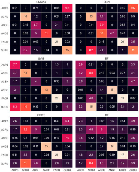
Figure 6.
Confusion matrices for comparison models. Rows and columns indicate correct and predicted labels, respectively. For data sources of these species, refer to Table 1. The value of each species is the average prediction of 100 models of each method.
CNN2C outperformed the other models on ACRU, FACR, QURU prediction, with 88.9%, 100%, and 65.2% precision, respectively (Table 6). DCN and SVM had the second best prediction on ACRU, both with 72.2% precision, 23.1% lower than CNN2C. SVM had the second-best prediction on FACR, with 95.8% precision, and DCN was second best on QURU, with 47.8% precision. CNN2C, DCN, and SVM showed more clear advantages in ACRU identification than the other conventional models. CNN2C was the only model that could identify QURU better than a random prediction. DCN and conventional models had significant difficulties separating QURU from ACRU (Figure 6).
Table 6.
Correct prediction ratio for comparison methods in application phase (%).
CNN2C performed second best on ACSH, with 74.4% precision, while DCN was the best, at 87.8%. Conventional models had significant difficulties separating ACSH from other species (Figure 6). No neural network model could identify ACPS. CNN2C and DCN tended to predict ACPS as QURU (Figure 6). SVM had a correct prediction ratio of 77% on ACPS, which outperformed the other models.
4. Discussion and Future Work
4.1. Reshaping Leaf Spectroscopy Data to Feed CNN Models
CNN models have been successfully applied since the early 2000 s to detect, segment, and recognize objects and regions in images [51]. While it is common to use CNN models to classify vegetation species from hyperspectral image data [17,18,52], little research has made full use of leaf spectroscopy data on species classification together with CNN models, which cannot use this 1D data. As a result, species classification based on leaf-level reflectance data relies more on ANNs and other conventional models, which use structured input data. Although there have been attempts to use 1D leaf spectroscopy data as the input for a CNN model [21], few studies have reshaped structural leaf spectroscopy data into 2D image data to feed a CNN model.
In this study, we have combined leaf scale spectroscopy data and a CNN model, whose superior performance, whether in the training or application phase, suggests its feasibility. There are noticeable differences in leaf pigments, cell structures, and water content among the samples in the dataset (Figure 7A). The DCN and conventional models should have learned these differences from the structured reflectance data to discriminate species. However, these differences are limited to one dimension (vertical in Figure 7A), and minor differences from other dimensions were ignored. When the reflectance data were reshaped into a 2D image, the differences could have been scaled in both the vertical and horizontal dimensions (Figure 7B). Thus, the differences between species can be exaggerated from a line to a surface (Figure 8). As a result, CNN models using these images may learn more unique features of each species and discriminate them well. The high performance in the application phase may also indicate that the learned features are more general for each species than in the DCN and conventional models, resulting in the unseen data also being more correctly identified.
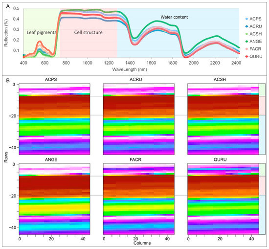
Figure 7.
Average reflectance and respective reshaped 2D images of six species. Grey images are colorized for better understanding of reflectance for the reader. (A) structure reflectance curve; (B) reshaped images (45 × 45).
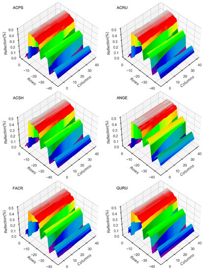
Figure 8.
Average reflectance image-stretched 3D charts of six species. Reshaped grey images are stretched into 3D charts and colorized. Differences in structured data are one vertical dimension; while being reshaped into a 2D image, differences between lines will be scaled into a surface. Thus, CNN models may learn more features from image data than DCN and conventional models, which use 1D structured data.
4.2. Superiority of CNN Model on Species Classification Using Leaf Spectroscopy Data
The results clearly show that in the training phase, the CNN model had the best validation accuracy. Furthermore, in the application phase, the CNN model, with two Conv layers, each with a pooling layer (CNN2C), had the best identification accuracy and precision. The high performance of CNN models in the training phase shows that they could perfectly discriminate six species, and only SVM could perform comparably among the conventional models. The advantage of the CNN model, however, is more apparent in the application phase. Thus, using 2D reshaped reflectance image data, the CNN model may be more general for unseen leaf reflectance data discrimination and have more application value for plant species identification.
Furthermore, the CNN2C model well separated ACRU, FACR, and QURU. Surprisingly, although all neural network models had difficulty distinguishing between ACPS and QURU, SVM performed much better. It is noticed that the ACPS training data were from ANGERS, using an ASD Field Spec spectroradiometer, while the identification data were from LOPEX93, using a Spectral Evolution PSR+ spectroradiometer. To determine whether the difference in instruments caused the problem, we excluded the five LOPEX93 QURU data items from the prediction dataset, and reinvestigated the application phase for the CNN2C model. The results showed that the correctly predicted QURU decreased from 15 (Figure 6 CNN2C) to 10 (Figure 9), 6.1 out of 23 QURU were still predicted as ACRU. This means that neither the different datasets nor the difference in instruments caused the problem, and that the CNN models may have learned characters similar to ACRU and QURU, finally causing the misidentification of QURU. More examination may be necessary.
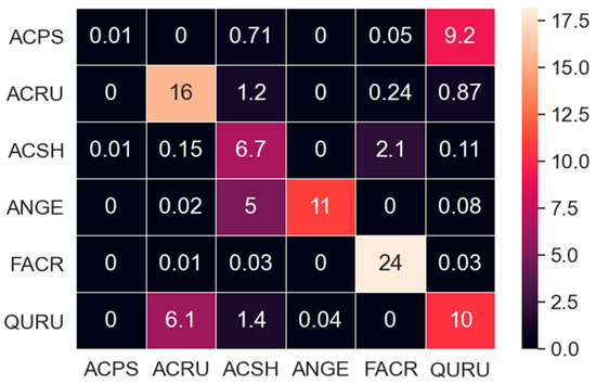
Figure 9.
Identification results of CNN2C for prediction of data without LO QURU data.
4.3. Advantages and Uncertainty of Approach; Future Studies
Most studies followed data-driven approaches and pursued an optimization of classification accuracy, while a concrete hypothesis or a targeted application was missing in all but a few exceptional studies [23]. The data from different locations or time periods were used as the unseen prediction data for the trained model. The CNN2C model performs best in this application phase. Although SVM performed as well as CNN2C in the training phase, it had difficulty identifying ACSH and QURU, clearly indicating that models established from data-driven approaches may only perform well in the training phase but not for unseen data, and may not find use in further species identification applications. Alternatively, CNN2C may be a more general model for species identification based on hyperspectral data.
Several sources of uncertainty remain. Compared with previous work, e.g., 46 species in Prospere et al. [13], 33 species in Kalacska et al. [53], and 40 species in Bahrami and Mobasheri [54], we had only six species, unfortunately, as the only ones with more than 80 samples in five datasets, while Beamlab [36] suggested that 100–1000 samples should be used in deep learning. Thirty species with fewer than 80 and more than 30 reflectance samples were not included, and whether these samples of small sizes affect the classification results was not examined. Thus, more experiments should be conducted, or leaf reflectance data of more species should be collected.
Similarly to the square images that are commonly used to feed CNNs, we reshaped 2025 reflectance features into 45 × 45 images for both training and prediction. To determine whether square-shaped image reflectance data are preferable, we used 14 differently shaped images (Figure 10) for CNN models. Results showed that the image in Figure 10j obtained higher prediction accuracy and precision for CNN2C, with an F1-score of 0.68. The image in Figure 10k obtained much better prediction accuracy and precision for CNN2 and CNN3. We may conclude that a square leaf hyperspectral image is not necessarily the best, and a tall, narrow rectangle shape may provide better results for deeper CNN models in species classification problems. The shapes of reflectance data for different CNN models should be carefully studied.
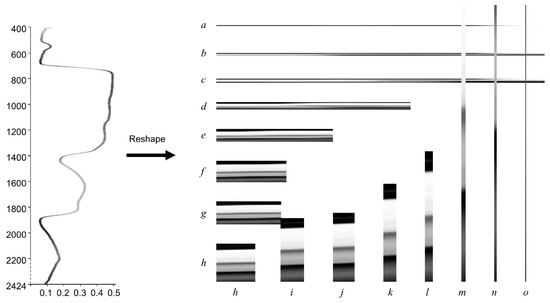
Figure 10.
Sample of a reshaped full wavelength reflectance structure data item. Reflectance wavelengths range from 400 to 2424 nm, and 2025 features are selected. There are 15 factors of 2025 (1, 3, 5, 9, 15, 25, 27, 45, 75, 81, 135, 225, 405, 675, 2025), so the image shape will be: (a) 1 × 2025; (b) 3 × 675; (c) 5 × 405; (d) 9 × 225; (e) 15 × 135; (f) 25 × 81; (g) 27 × 75; (h) 45 × 45 (Figure 3); (i) 75 × 27; (j) 81 × 25; (k) 135 × 15; (l) 225 × 9; (m) 405 × 5; (n) 675 × 3; (o) 2025 × 1 pixels. Each image shape will generate a new dataset to feed the CNN models. Image shapes of (a, b, c, m, n, and o) are not fully demonstrated, as they are either too wide or too tall.
Unlike studies that use wavelength selection preprocessing to downscale the training dataset, we adopted almost the full domain of reflectance data; whether the downscaled data affect the classification results is still unknown. Additionally, compared to other traditional methods, the proposed method of this study requires more time during the procedure, thus some improvements could be carried out in future studies. Overall, we attempted to reshape 1D reflectance data into 2D image reflectance data to feed a CNN, and showed that it could effectively classify and identify six species from different locations. The approach can be extended to estimate other leaf traits.
5. Conclusions
We reshaped 1D leaf-level reflectance data into a 2D grey image and presented a workflow for tree species classification from hyperspectral data to produce an end-to-end classification method. We compared the performance of eight feedforward neural network architectures, a DCN, SVM, RF, a gradient boosting machine, and a DT model for this task. The study showed that species identification can be conducted with high accuracy with the given methods and 2D image data. The implemented CNN2C was the best model, outperforming DCN, SVM, RF, GBDT, and DT in the application phase. We aim to use 2D image data instead of 1D structure data to feed CNN models and simulate an application phase to produce a general model for comprehensive data source classification tasks. Developing these methods is crucial for the use of leaf levels and remote sensing hyperspectral data, which are projected to become increasingly available in the future, for large-scale biodiversity monitoring.
Supplementary Materials
The following supporting information can be downloaded at: https://www.mdpi.com/article/10.3390/rs14163972/s1, Figure S1: Prediction confusion matrices for different SVM kernels, linear, poly, RBF, and sigmoid; Figure S2: Prediction confusion matrices for CNN models.
Author Contributions
Methodology, writing—original draft preparation, S.Y.; validation, writing—review and editing, G.S.; supervision, G.H.; conceptualization, writing—review and editing, supervision, Q.W. All authors have read and agreed to the published version of the manuscript.
Funding
This research was partially supported by Science and Technology Planning Project of Guangdong Province (2020B121201013) and Guangdong Academy of Sciences (2020GDASYL-20200301003).
Data Availability Statement
The data that support the findings of this study are available on request from the corresponding author.
Acknowledgments
We gratefully acknowledge the open access to the TensorFlow CNN model and the Ecological Spectral Information System for open datasets.
Conflicts of Interest
The authors declare no conflict of interest.
References
- Wäldchen, J.; Mäder, P. Plant Species Identification Using Computer Vision Techniques: A Systematic Literature Review; Springer: Dordrecht, The Netherlands, 2018; Volume 25, ISBN 0123456789. [Google Scholar]
- Hassoon, I.M.; Kassir, S.A.; Altaie, S.M. A review of plant species identification techniques. Int. J. Sci. Res. 2018, 7, 325–328. [Google Scholar]
- Cope, J.S.; Corney, D.; Clark, J.Y.; Remagnino, P.; Wilkin, P. Plant species identification using digital morphometrics: A review. Expert Syst. Appl. 2012, 39, 7562–7573. [Google Scholar] [CrossRef]
- Wäldchen, J.; Rzanny, M.; Seeland, M.; Mäder, P. Automated plant species identification—Trends and future directions. PLoS Comput. Biol. 2018, 14, e1005993. [Google Scholar] [CrossRef]
- Lee, S.H.; Chan, C.S.; Wilkin, P.; Remagnino, P. Deep-Plant: Plant identification with convolutional neural networks. In Proceedings of the 2015 IEEE International Conference on Image Processing (ICIP), Quebec City, QC, Canada, 27 September–1 October 2015; pp. 452–456. [Google Scholar]
- Lee, S.H.; Chan, C.S.; Mayo, S.J.; Remagnino, P. How deep learning extracts and learns leaf features for plant classification. Pattern Recognit. 2017, 71, 1–13. [Google Scholar] [CrossRef]
- Zhang, C.; Zhou, P.; Li, C.; Liu, L. A convolutional neural network for leaves recognition using data augmentation. In Proceedings of the 2015 IEEE International Conference on Computer and Information Technology, Ubiquitous Computing and Communications, Dependable, Autonomic and Secure Computing, Pervasive Intelligence and Computing, Liverpool, UK, 26–28 October 2015; pp. 2143–2150. [Google Scholar]
- Castro-Esau, K.L.; Sánchez-Azofeifa, G.A.; Caelli, T. Discrimination of lianas and trees with leaf-level hyperspectral data. Remote Sens. Environ. 2004, 90, 353–372. [Google Scholar] [CrossRef]
- Chan, J.C.-W.; Paelinckx, D. Evaluation of random forest and adaboost tree-based ensemble classification and spectral band selection for ecotope mapping using airborne hyperspectral imagery. Remote Sens. Environ. 2008, 112, 2999–3011. [Google Scholar] [CrossRef]
- Clark, M.L.; Roberts, D.A.; Clark, D.B. Hyperspectral discrimination of tropical rain forest tree species at leaf to crown scales. Remote Sens. Environ. 2005, 96, 375–398. [Google Scholar] [CrossRef]
- Ferreira, M.P.; Zortea, M.; Zanotta, D.C.; Shimabukuro, Y.E.; de Souza Filho, C.R. Mapping tree species in tropical seasonal semi-deciduous forests with hyperspectral and multispectral data. Remote Sens. Environ. 2016, 179, 66–78. [Google Scholar] [CrossRef]
- Kishore, B.S.P.C.; Kumar, A.; Saikia, P.; Lele, N.V.; Pandey, A.C.; Srivastava, P.; Bhattacharya, B.K.; Khan, M.L. Major forests and plant species discrimination in Mudumalai forest region using airborne hyperspectral sensing. J. Asia-Pac. Biodivers. 2020, 13, 637–651. [Google Scholar] [CrossRef]
- Prospere, K.; McLaren, K.; Wilson, B. Plant species discrimination in a tropical wetland using in situ hyperspectral data. Remote Sens. 2014, 6, 8494–8523. [Google Scholar] [CrossRef]
- Long, Y.; Rivard, B.; Sanchez-Azofeifa, A.; Greiner, R.; Harrison, D.; Jia, S. Identification of spectral features in the longwave infrared (LWIR) spectra of leaves for the discrimination of tropical dry forest tree species. Int. J. Appl. Earth Obs. Geoinf. 2021, 97, 102286. [Google Scholar] [CrossRef]
- Gong, P.; Ruilianp, P.; Bin, Y. Conifer species recognition: An exploratory analysis of in situ hyperspectral data. Remote Sens. Environ. 1997, 62, 189–200. [Google Scholar] [CrossRef]
- Roth, K.L.; Roberts, D.A.; Dennison, P.E.; Peterson, S.H.; Alonzo, M. The impact of spatial resolution on the classification of plant species and functional types within imaging spectrometer data. Remote Sens. Environ. 2015, 171, 45–57. [Google Scholar] [CrossRef]
- Mäyrä, J.; Keski-Saari, S.; Kivinen, S.; Tanhuanpää, T.; Hurskainen, P.; Kullberg, P.; Poikolainen, L.; Viinikka, A.; Tuominen, S.; Kumpula, T.; et al. Tree species classification from airborne hyperspectral and LiDAR data using 3D convolutional neural networks. Remote Sens. Environ. 2021, 256, 112322. [Google Scholar] [CrossRef]
- Zhang, B.; Zhao, L.; Zhang, X. Three-dimensional convolutional neural network model for tree species classification using airborne hyperspectral images. Remote Sens. Environ. 2020, 247, 111938. [Google Scholar] [CrossRef]
- Hennessy, A.; Clarke, K.; Lewis, M. Hyperspectral classification of plants: A review of waveband selection generalisability. Remote Sens. 2020, 12, 113. [Google Scholar] [CrossRef]
- Khdery, G.A.; Farg, E.; Arafat, S.M. Natural vegetation cover analysis in Wadi Hagul, Egypt using hyperspectral remote sensing approach. Egypt. J. Remote Sens. Space Sci. 2019, 22, 253–262. [Google Scholar] [CrossRef]
- Jernelv, I.L.; Hjelme, D.R.; Matsuura, Y.; Aksnes, A. Convolutional neural networks for classification and regression analysis of one-dimensional spectral data. arXiv 2020, arXiv:2005.07530. [Google Scholar]
- Krizhevsky, A.; Sutskever, I.; Hinton, G.E. Imagenet classification with deep convolutional neural networks. Adv. Neural Inf. Process. Sust. 2012, 25. Available online: https://proceedings.neurips.cc/paper/2012/hash/c399862d3b9d6b76c8436e924a68c45b-Abstract.html (accessed on 5 February 2021). [CrossRef]
- Fassnacht, F.E.; Latifi, H.; Stereńczak, K.; Modzelewska, A.; Lefsky, M.; Waser, L.T.; Straub, C.; Ghosh, A. Review of studies on tree species classification from remotely sensed data. Remote Sens. Environ. 2016, 186, 64–87. [Google Scholar] [CrossRef]
- Sims, D.A.; Gamon, J.A. Relationships between leaf pigment content and spectral reflectance across a wide range of species, leaf structures and developmental stages. Remote Sens. Environ. 2002, 81, 337–354. [Google Scholar] [CrossRef]
- Jacquemoud, S.; Ustin, S.L.; Verdebout, J.; Schmuck, G.; Andreoli, G.; Hosgood, B. Estimating leaf biochemistry using the PROSPECT leaf optical properties model. Remote Sens. Environ. 1996, 56, 194–202. [Google Scholar] [CrossRef]
- Wang, Z.; Townsend, P.A.; Schweiger, A.K.; Couture, J.J.; Singh, A.; Hobbie, S.E.; Cavender-Bares, J. Mapping foliar functional traits and their uncertainties across three years in a grassland experiment. Remote Sens. Environ. 2019, 221, 405–416. [Google Scholar] [CrossRef]
- Meireles, J.E.; Cavender-Bares, J.; Townsend, P.A.; Ustin, S.; Gamon, J.A.; Schweiger, A.K.; Schaepman, M.E.; Asner, G.P.; Martin, R.E.; Singh, A.; et al. Leaf reflectance spectra capture the evolutionary history of seed plants. New Phytol. 2020, 228, 485–493. [Google Scholar] [CrossRef]
- Chen, J.; Pisonero, J.; Chen, S.; Wang, X.; Fan, Q.; Duan, Y. Convolutional neural network as a novel classification approach for laser-induced breakdown spectroscopy applications in lithological recognition. Spectrochim. Acta Part B At. Spectrosc. 2020, 166, 105801. [Google Scholar] [CrossRef]
- Gao, H.; Yang, Y.; Li, C.; Zhou, H.; Qu, X. Joint alternate small convolution and feature reuse for hyperspectral image classification. ISPRS Int. J. Geo-Inf. 2018, 7, 349. [Google Scholar] [CrossRef]
- Lumini, A.; Nanni, L. Convolutional neural networks for ATC classification. Curr. Pharm. Des. 2018, 24, 4007–4012. [Google Scholar] [CrossRef]
- Yang, W.; Nigon, T.; Hao, Z.; Paiao, G.D.; Fernández, F.G.; Mulla, D.; Yang, C. Estimation of corn yield based on hyperspectral imagery and convolutional neural network. Comput. Electron. Agric. 2021, 184, 106092. [Google Scholar] [CrossRef]
- Luo, Y.; Zou, J.; Yao, C.; Zhao, X.; Li, T.; Bai, G. HSI-CNN: A novel convolution neural network for hyperspectral image. In Proceedings of the ICALIP 2018 6th International Conference on Audio, Language and Image Processing, Shanghai, China, 16–17 July 2018; IEEE: Piscataway, NJ, USA, 2018; pp. 464–469. [Google Scholar]
- Han, Z.; Gao, J. Pixel-level aflatoxin detecting based on deep learning and hyperspectral imaging. Comput. Electron. Agric. 2019, 164, 104888. [Google Scholar] [CrossRef]
- Wang, Z. Fresh Leaf Spectra to Estimate LMA over NEON Domains in Eastern United States. Available online: https://ecosis.org/package/fresh-leaf-spectra-to-estimate-lma-over-neon-domains-in-eastern-united-states (accessed on 5 February 2021).
- Kothari, S.; Montgomery, R.; Cavender-Bares, J. FAB Leaf Spectra across a Light Gradient at Cedar Creek LTER. Available online: https://ecosis.org/package/fab-leaf-spectra-across-a-light-gradient-at-cedar-creek-lter (accessed on 5 February 2021).
- Beamlab You Can Probably Use Deep Learning Even If Your Data Isn’t That Big. Available online: https://beamandrew.github.io/deeplearning/2017/06/04/deep_learning_works.html (accessed on 30 June 2021).
- Srivastava, N.; Hinton, G.; Krizhevsky, A.; Sutskever, I.; Salakhutdinov, R. Dropout: A simple way to prevent neural networks from overfitting. J. Mach. Learn. Res. 2014, 15, 1929–1958. [Google Scholar]
- Xu, B.; Wang, N.; Chen, T.; Li, M. Empirical evaluation of rectified activations in convolutional network. arXiv 2015, arXiv:1505.00853. [Google Scholar]
- Kingma, D.P.; Ba, J.L. Adam: A method for stochastic optimization. In Proceedings of the 3rd International Conference on Learning Representations (ICLR 2015), Conference Track Proceedings, San Diego, CA, USA, 7–9 May 2015; pp. 1–15. [Google Scholar]
- Wang, R.; Fu, G.; Fu, B.; Wang, M. Deep & cross network for ad click predictions. In Proceedings of the 2017 AdKDD TargetAd—In Conjunction with the 23rd ACM SIGKDD Conference on Knowledge Discovery and Data Mining (KDD 2017), Halifax, NS, Canada, 13–17 August 2017. [Google Scholar]
- Wang, R.; Shivanna, R.; Cheng, D.; Jain, S.; Lin, D.; Hong, L.; Chi, E. DCN V2: Improved Deep & Cross Network and Practical Lessons for Web-Scale Learning to Rank Systems; Association for Computing Machinery: New York, NY, USA, 2020; ISBN 9781450383127. [Google Scholar]
- Khalid, S. Structured Data Learning with Wide, Deep, and Cross Networks. Available online: https://keras.io/examples/structured_data/wide_deep_cross_networks/#experiment-3-deep-amp-cross-model (accessed on 3 July 2021).
- Abadi, M.; Agarwal, A.; Barham, P.; Brevdo, E.; Chen, Z.; Citro, C.; Corrado, G.S.; Davis, A.; Dean, J.; Devin, M.; et al. TensorFlow: Large-scale machine learning on heterogeneous distributed systems. arXiv 2016, arXiv:1603.04467. [Google Scholar]
- Pedregosa, F.; Varoquaux, G.; Gramfort, A.; Michel, V.; Thirion, B.; Grisel, O.; Blondel, M.; Prettenhofer, P.; Weiss, R.; Dubourg, V.; et al. Scikit-Learn: Machine learning in Python. J. Mach. Learn. Res. 2011, 12, 2825–2830. [Google Scholar]
- Mountrakis, G.; Im, J.; Ogole, C. Support vector machines in remote sensing: A review. ISPRS J. Photogramm. Remote Sens. 2011, 66, 247–259. [Google Scholar] [CrossRef]
- Mantero, P.; Moser, G.; Serpico, S.B. Partially supervised classification of remote sensing images using SVM-based probability density estimation. IEEE Trans. Geosci. Remote Sens. 2005, 43, 559–570. [Google Scholar] [CrossRef]
- Somvanshi, M.; Chavan, P.; Tambade, S.; Shinde, S.V. A review of machine learning techniques using decision tree and support vector machine. In Proceedings of the 2nd International Conference on Computing Communication Control and Automation (ICCUBEA), Pune, India, 12–13 August 2016. [Google Scholar] [CrossRef]
- Yang, C.-C.; Prasher, S.O.; Enright, P.; Madramootoo, C.; Burgess, M.; Goel, P.K.; Callum, I. Application of decision tree technology for image classification using remote sensing data. Agric. Syst. 2003, 76, 1101–1117. [Google Scholar] [CrossRef]
- Natekin, A.; Knoll, A. Gradient boosting machines, a tutorial. Front. Neurorobot. 2013, 7, 21. [Google Scholar] [CrossRef] [PubMed]
- Jin, X.; Jie, L.; Wang, S.; Qi, H.J.; Li, S.W. Classifying wheat hyperspectral pixels of healthy heads and fusarium head blight disease using a deep neural network in the wild field. Remote Sens. 2018, 10, 395. [Google Scholar] [CrossRef]
- Lecun, Y.; Bengio, Y.; Hinton, G. Deep learning. Nature 2015, 521, 436–444. [Google Scholar] [CrossRef]
- Fricker, G.A.; Ventura, J.D.; Wolf, J.A.; North, M.P.; Davis, F.W.; Franklin, J. A convolutional neural network classifier identifies tree species in mixed-conifer forest from hyperspectral imagery. Remote Sens. 2019, 11, 2326. [Google Scholar] [CrossRef]
- Kalacska, M.; Bohlman, S.; Sanchez-Azofeifa, G.; Castro-Esau, K.; Caelli, T. Hyperspectral discrimination of tropical dry forest lianas and trees: Comparative data reduction approaches at the leaf and canopy levels. Remote Sens. Environ. 2007, 109, 406–415. [Google Scholar] [CrossRef]
- Bahrami, M.; Mobasheri, M.R. Plant species determination by coding leaf reflectance spectrum and its derivatives. Eur. J. Remote Sens. 2020, 53, 258–273. [Google Scholar] [CrossRef]
Publisher’s Note: MDPI stays neutral with regard to jurisdictional claims in published maps and institutional affiliations. |
© 2022 by the authors. Licensee MDPI, Basel, Switzerland. This article is an open access article distributed under the terms and conditions of the Creative Commons Attribution (CC BY) license (https://creativecommons.org/licenses/by/4.0/).