Article

Genetic Algorithm Captured the Informative Bands for Partial Least Squares Regression Better on Retrieving Leaf Nitrogen from Hyperspectral Reflectance

1
Key Laboratory of Environment Change and Resources Use in Beibu Gulf, Ministry of Education, Nanning Normal University, Nanning 530001, China
2
College of Geography and Environmental Sciences, Zhejiang Normal University, Jinhua 321004, China
3
Faculty of Agriculture, Shizuoka University, Shizuoka 422-8529, Japan
*
Author to whom correspondence should be addressed.
Remote Sens. 2022, 14(20), 5204; https://doi.org/10.3390/rs14205204
Submission received: 5 September 2022 / Revised: 11 October 2022 / Accepted: 13 October 2022 / Published: 18 October 2022
(This article belongs to the Special Issue Hyperspectral Remote Sensing of Vegetation Functions)

Abstract

:
Nitrogen is a major nutrient regulating the physiological processes of plants. Although various partial least squares regression (PLSR) models have been proposed to estimate the leaf nitrogen content (LNC) from hyperspectral data with good accuracies, they are unfortunately not robust and are often not applicable to novel datasets beyond which they were developed. Selecting informative bands has been reported to be critical to refining the performance of the PLSR model and improving its robustness for general applications. However, no consensus on the optimal band selection method has yet been reached because the calibration and validation datasets are very often limited to a few species with small sample sizes. In this study, we address the question based on a relatively comprehensive joint dataset, including a simulation dataset generated from the recently developed leaf scale radiative transfer model (PROSPECT-PRO) and two public online datasets, for assessing different informative band selection techniques on the informative band selection. The results revealed that the goodness-of-fit of PLSR models to estimate LNC could be greatly improved by coupling appropriate band-selection methods rather than using full bands instead. The PLSR models calibrated from the simulation dataset with informative bands selected by genetic algorithm (GA) and uninformative variable elimination (UVE) method were reliable for retrieving the LNC of the two independent field-measured datasets as well. Particularly, GA was more effective to capture the informative bands for retrieving LNC from hyperspectral data. These findings should provide valuable insights for building robust PLSR models for retrieving LNC from hyperspectral remote sensing data.

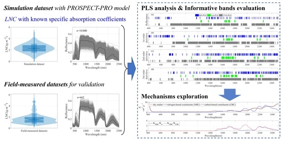
Graphical Abstract

1. Introduction

Nitrogen is a major nutrient regulating the physiological processes of plants [1]; its content is closely related to the photosynthetic capacity of leaves [2], therefore strongly influencing the yield and quality in terms of crops [3]. Unfortunately, the leaf nitrogen content (LNC) in plants is highly variable in different leaf developmental stages and light environments [1,4], making traditional destructive measurements (which require tissue sampling and laboratory analysis) in general unable to catch the dynamic process up. Thus, an efficient and non-destructive measurement of plant LNC is highly desired for a better understanding of ecosystem functional dynamics [4].
Among various currently prevalent approaches, hyperspectral remote sensing has emerged as a premier choice for retrieving plant biochemical and biophysical traits, also including LNC, at broad spatial scales in the last few decades [5,6,7,8]. It is becoming clear that the successful applications of plant-trait estimation from hyperspectral data rely heavily on the full understanding of light interaction with plant traits and interpretability of the reflectance data under different plant-trait conditions [1]. While the physical-law-based radiative transfer models (RTMs) provide more robust retrievals of leaf traits [9,10], the inversion retrievals using RTMs usually face serious ill-posed problems [11]; thus, statistical approaches remain popular choices.
Up to now, various statistical-based methods, such as hyperspectral index, partial least squares regression (PLSR), machine learning (ML), etc., have been developed to estimate LNC from hyperspectral data [1,5,12,13,14,15,16]. Among them, the partial least squares (PLS) regression is known to be suitable for analyzing multi-collinear and high-dimensional spectral data [17,18,19]. As a truth, many results demonstrated that PLS outperformed other traditional regression techniques in retrieving various leaf biochemical contents [18,20,21,22]. However, LNC is a much more difficult leaf trait to capture due to the interactions between nitrogen and carbon-based constituents, water, and pigments [1,23]. Furthermore, most models were calibrated from specific datasets, making them usually perform well only on the training datasets but lose the generalization when implemented on a new dataset [1,24,25,26]. Hence, it is necessary for a robust method to be developed to reduce its uncertainty while improving its generalization in the assessment of LNC from leaf reflectance.
While a good way to build a universal model would always be to use a large database covering as many plant leaf conditions as possible [24], limited available resources frequently lead to a large volume of data being unreachable. Alternatively, RTMs can model endless variations of reflectance by changing model input parameters and thus would allow us to build a large database covering various plant nitrogen-based constituent conditions.
Another big issue affecting the robustness of PLSR to retrieve plant traits from hyperspectral data is how to select informative spectral bands among all hyperspectral bands [17,27,28,29]. It has been proved that selecting informative bands is critical to refining the performance of PLS analysis [17] and improving its robustness for general applications [30,31]. Despite many techniques, such as stepwise regression, uninformative variable elimination (UVE), and genetic algorithm (GA), that have been proposed to select informative spectral bands (or eliminate uninformative bands) for PLS regression analyses [17,29,30,32,33,34], most reported PLSR models unfortunately still used full bands for LNC estimation [1,4,5,14,16,35,36,37,38]. Only a limited number of them have investigated their performance based on selected wavelengths [39]. Furthermore, most proposed PLSR models, even coupled with informative band selection, are usually built up from specific field datasets and are trained to catch up with local features frequently, which seriously refrains their applications into new areas. In addition, their used bands are usually hard to be explained theoretically. On the other hand, RTM-based simulations are typical with explainable mechanisms and thus provide a much more straightforward and strict validation of different band selection techniques.
Furthermore, reported PLSR models used very different wavelength domains, e.g., 350–1800 nm for wheat LNC estimation [38], 400–1050 nm for estimating LNC in winter wheat [37], 400–1700 nm for the prediction of LNC in forest litterfall samples [39], 400–2200 nm to capture the seasonal variability of LNC at two temperate deciduous forests [4], 500–2400 nm to predict LNC in crops [14,16], 550–2300 nm for LNC estimation across different plant species [1], and 1500–2400 nm for the foliar nitrogen concentration of temperate and boreal tree species estimation [2]; it is thus worth noting whether such different wavelength domains have certain impacts on their robustness.
In addition, spectral transformation techniques are commonly used to reduce the effects of baseline shifts and noises in hyperspectral multivariate regression analyses (including PLSR) [39,40]. Derivatives are among the most commonly used data-transformation techniques as derivative-based analyses can extract the absorption band positions from reflectance spectra [41,42,43] and resolve overlapping spectral features [44,45]. We therefore attempt to combine derivatives with PLSR modeling to take the usage of their resistance to various noises.
Thus, the specific objectives of this study are: (1) to build up PLSR models for retrieving LNC from a simulation dataset with a large volume of sample size by coupling with different informative band selection techniques and verifying their performance using two independent measured datasets; (2) to provide an explanation for the mechanism for selected bands; and (3) to assess PLSR models built up from different wavelength domains. Following the aforementioned strategy, we used the recently developed PROSPECT-PRO which separated the nitrogen-based constituents (proteins) from carbon-based constituents [3] to produce a rather comprehensive dataset for assessing different informative band selection techniques. The robustness of the developed PLSR models was further validated using two publicly available field datasets.

2. Materials and Methods

2.1. Datasets for LNC and Leaf Reflectance

The PROSPECT-PRO model [3], which was newly developed on the basis of the well-accepted leaf scale radiative transfer model PROSPECT [46], was applied to generate the base dataset used in this study. In PROSPECT-PRO, the leaf reflectance (400–2500 nm) is calculated from the leaf structure coefficient, leaf pigment contents (chlorophyll, carotenoid, anthocyanin, and brown pigment), leaf water content, leaf mass area, protein content, and carbon-based constituents. The PROSPECT-PRO model has separated the nitrogen-based constituents (proteins) from carbon-based constituents, enabling us to generate a large leaf optical simulation dataset with various leaf nitrogen contents. In order to maintain the actual correlations between leaf constituents, we adopted the sampling strategy proposed by Féret et al. (2011) to generate the model input parameters for the simulation dataset in this study [25]. In detail, the covariations between leaf biochemical parameters were calculated from the LOPEX leaf optical properties database [47]. The anthocyanin content and brown pigment content were set to 0 as they exhibited low contents in leaves and had no overlap absorption effects to LNC. A total of 10,000 leaf spectra were simulated with input parameter combinations produced using the Latin hypercube sampling method [48]. The LNC values were calculated from the nitrogen-based constituents using the suggested nitrogen-to-crude protein conversion factor of 4.43 [3].
The distribution details of LNC in different datasets used in this study are illustrated in Figure 1. In the simulation dataset, the LNC followed a normal distribution with a mean value of 2.30 g m−2 and a standard deviation of 0.80 g m−2.
Two online datasets were used as validation datasets in this study. In dataset A, a total of 183 leaf samples with synchronous measurements of leaf nitrogen content (LNC, g m−2) and leaf reflectance of eight crop species (common sunflower, cottonwood, field pumpkin, garden cucumber, garden tomato, kidney bean, soybean, and sweet basil) were available at https://doi.org/10.21232/C2GM2Z accessed on 4 September 2022 [49]. In dataset B, leaf spectral and biochemical data of seven crops (Carolina poplar, cayenne pepper, common sunflower, cultivated radish, field pumpkin, foxtail millet, and sorghum) were provided (available at https://doi.org/10.21232/UTK8zaW4 accessed on 4 September 2022). In this study, we used 479 samples with synchronous measurements of the leaf nitrogen content (g m−2) and leaf reflectance [50]. In dataset A, the mean value and standard deviation of LNC were 1.21 g m−2 and 0.51 g m−2, respectively. In dataset B, the mean value and standard deviation of LNC were 1.87 g m−2 and 1.04 g m−2, respectively. Larger standard deviations of LNC were found in dataset B, which were collected for watered and droughted crops in drought experiments. For all field-measured leaf samples in datasets A and B, the mean value and standard deviation of LNC were 1.68 g m−2 and 0.97 g m−2, respectively.
All the leaf spectra in the simulation dataset and the two field-measured datasets are illustrated in Figure 2. The average reflectance in three datasets exhibited similar patterns. Leaf reflectance values within 400–700 nm and 1400–2500 nm were low due to the absorption of leaf components including pigments, water, nitrogen, protein, lignin, cellulose, and others. Leaf reflectance values within 700–1400 nm were large because they lacked strong absorption features. However, leaf spectra in dataset B were collected for watered and droughted crops in drought experiments. As a result, the reflectance values exhibited larger variations than those of dataset A, especially around the wavelengths near 1000 nm, 1700 nm, and 2200 nm.

2.2. Spectral Data Processing

An overall range of 400–2500 nm was used for PLS analysis in this study. The reflectance of each leaf sample was smoothed with the five-point centered moving average method for removing noise [51]. For computational efficiency, the reflectance recorded in the dataset at the 1 nm spectral resolution was resampled to 5 nm. In addition to reflectance, derivatives were also calculated to reduce the effects of baseline shifts and noises in hyperspectral PLSR analysis [41,42,43]. The 1st- to 3rd-order derivative spectra were then calculated from the resampled 5 nm-resolution spectra. The derivative at wavelength i was calculated according to the “finite divided difference approximation” method [43,52]:
d λ i = ds d λ | i s ( λ i + 1 ) s ( λ i ) λ i + 1 λ i
where s(λi+1) and s(λi) are the values of the spectrum at wavelength i+1 and i, respectively, and λi+1–λi is the wavelength difference between the two bands.

2.3. Informative Band Selections and Partial Least Squares Regression Analyses

The PLSR analyses with different spectral transformations (raw reflectance and derivatives in this study) were conducted to estimate the LNC. In addition to using full available bands (FB-PLS), three commonly applied variable selection/elimination approaches were coupled for selecting informative bands for PLSR models. They are the iterative stepwise elimination (ISE-PLS) [17,53], the genetic algorithms developed by Leardi (2000) (GA-PLS) [54], and the uninformative variable elimination (UVE-PLS) [32].
Stepwise regression is a simple method to add or remove variables from a multilinear model based on the statistical significance of the variables [29]. To determine whether a variable should be included in the PLSR model, the p-value of an F-statistic is computed to test the model with and without this variable. The stepwise regressions were conducted using the built-in function (stepwisefit) of MATLAB (The MathWorks, Inc. Portola Valley, CA, USA). In this study, the p-value tolerance for adding spectral bands to the model was defined as 0.05 while the p-value tolerance for removing spectral bands from the model was defined as 0.10.
Genetic algorithms (GA) have been combined with PLS two decades ago [55]. The genetic algorithms have significant effects on band selection as the algorithms are developed based on biological evolutionary theory and natural selection [27]. The application of GA-PLS in this study was adopted from Leardi (2000). The online manual and source code of this method is available at http://www.models.life.ku.dk/GAPLS (accessed on 22 March 2020).
The UVE-PLS eliminated uninformative variables based on the reliability criterion of each variable [32]. The reliability criterion ( c λ ) of a certain band λ was first calculated based on the regression coefficients generated from FB-PLS as the ratio of the mean value of the regression coefficients and their standard deviation. Then, an artificial normally distributed random variable matrix with very small amplitude (1 × 10⁻⁵ in this study) was added to the original spectral data. The reliability criteria of these artificial variables were also calculated based on their regression coefficients of FB-PLS. Finally, the bands with absolute values of reliability criterion lower than the cutoff level (defined as the highest absolute value of the reliability criterion among all artificial variables) were eliminated [33]. More details of this method can be found in Centner et al. (1996) and Jin and Wang (2019).
The number of components (NoC) is critical for the performance of PLSR as overfitting may exist in PLSR with a large NoC [56]. To select the optimal number of components (NoC), PLSR models were first built for each of a series of NoC (from 1 to a maximum NoC). The maximum NoC in this study was restricted to 20 as suggested by Burnett et al. (2021) for fitting basic, leaf-level spectra-trait models [56]. For each NoC, the PLSR model was evaluated with k-fold cross-validation (where k = 5), which is commonly used to compare and select a model for a given predictive modeling problem [57]. In k-fold cross-validation (k = 5), the original sample is randomly partitioned into 5 equal-sized subsamples. Of the 5 subsamples, a single subsample is retained as the validation data for testing the PLSR model and the remaining 4 subsamples are used as modeling data to build the PLSR model. The root mean square errors (RMSEs) were calculated for both modeling and validation datasets and the same procedures were repeated 5 times to obtain the averaged RMSE values to evaluate the PLSR model. The optimal NoC is indicated by the minimum RMSE value.
PROSPECT-PRO considers that nitrogen-based constituents (proteins) only influence leaf spectral reflectance in the short-wave infrared (SWIR) range (1400–2500 nm) [3,58,59]; the simulation-dataset-rooted PLSR models trained from the wavelength domain shorter than 1400 nm are projected with poor performance since there is no informative band related to LNC theoretically. We have performed PLSR analyses at respective spectra regions (400–2500 nm, 400–1400 nm, and 1400–2500 nm) to investigate the performances of different band-selection methods on their capabilities of capturing informative bands for LNC estimation; targets for providing mechanical explanations for those informative bands being selected. The simulation dataset provides an ideal source to reach the goal since the radiative transfer background of each spectral band of the dataset is clearly known.

2.4. Model Performance Evaluation

The PLSR models were calibrated using the simulation dataset and validated with the other two independent field-measured datasets. The commonly used coefficient of determination (R2) and the normalized root mean square error (NRMSE, which is normalized by the mean value of the measurements) were calculated for both modeling and validation datasets to evaluate the model performance.
In addition, the corrected Akaike information criterion (AICc) provides a means for model selection and is ideal for minimizing the overfitting risk [60,61,62]. The AICc has been commonly used as an estimator of prediction error and relative quality of statistical models [63,64]. Thus, the goodness-of-fit (GoF) of a PLSR model was indicated by the AICc value which deals with the trade-off between the prediction accuracy and the simplicity of the model. The AICc is calculated as follows:
A I C c = ln R S S N + N + m N m 2
where N is the number of leaf samples, m is the number of model parameters (selected bands involved in PLSR models), and RSS is the residual sum of squares.

3. Results

3.1. LNC Estimation from Spectra within 1400–2500 nm Using PLSR Models

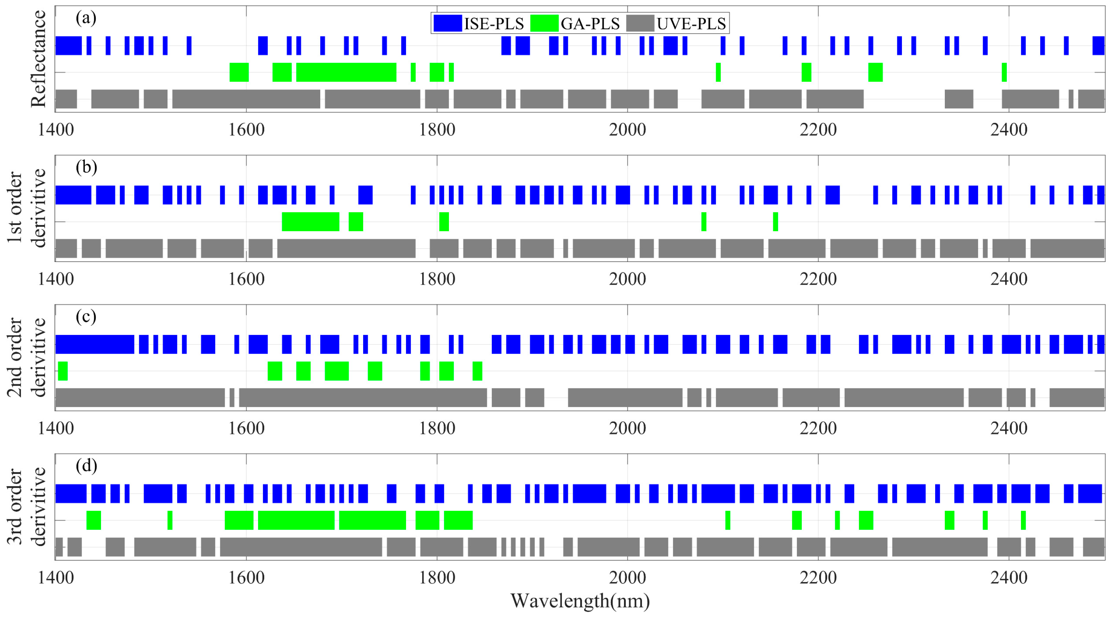
Using spectra within the known absorption region (1400–2500 nm) of nitrogen-based constituents (proteins), four different PLSR models using different preprocessed spectra were calibrated and validated to the simulation dataset for their performance in estimating LNC by coupling with different informative band selection approaches. Except for FB-PLS regression models, which used all bands within 1400–2500 nm, the informative bands selected for ISE-PLS, GA-PLS, and UVE-PLS regression models are illustrated in Figure 3. The results clearly indicated that ISE and UVE band-selection methods uniformly selected the wavelengths in the spectral region from 1400 to 2500 nm while much fewer bands were involved in GA-PLS regression models. Furthermore, the bands within 1600–1800 nm were identified as the most important bands for LNC estimation with PLSR models from all four spectral forms (irrespective of reflectance and derivatives).
The statistical criteria of each model were provided in Table 1. For FB-PLS regression models, all 221 bands within the range of 1400 to 2500 nm (at a 5 nm spectral resolution) were used for LNC estimation. Although all PLSR models closely captured (R2 > 0.96) the variation in LNC in the simulation dataset from which they were calibrated, the FB-PLS and ISE-PLS regression models exhibited low accuracies to trace the LNC in independent validation datasets (dataset A and dataset B). Compared with FB-PLS regression models, the GoFs of PLSR models combined with the GA and UVE band-selection methods to estimate LNC were greatly improved, as indicated by the much smaller AICc values. Even with a limited number of bands, the GA-PLS and UVE-PLS regression models were applicable for both independent validation datasets (dataset A and dataset B). Among the three band-selection methods, the GA-PLS regression models used the fewest bands for LNC estimation for all four different spectral transformations.

3.2. LNC Estimation from Spectra within 400–2500 nm Using PLSR Models

To further investigate the performances of different band-selection methods in eliminating uninformative bands which are not directly influenced by nitrogen-based constituents, we calibrated the PLSR model to estimate LNC with spectra covering from 400 to 2500 nm.
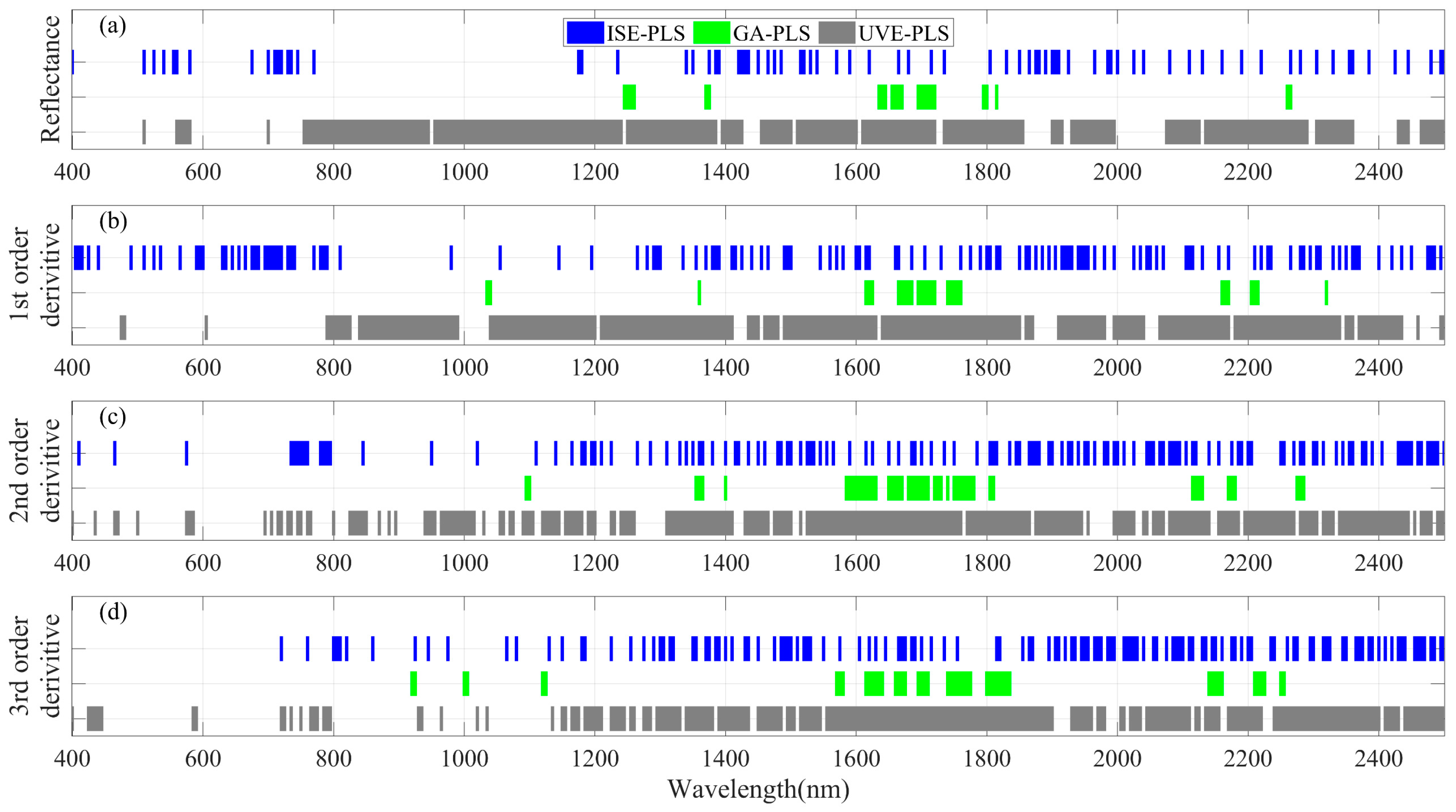
Even when the specific absorption coefficients of nitrogen-based constituents (proteins) within 400–1400 nm were neglected, many bands within this spectral region were unfortunately selected in ISE-PLS and UVE-PLS regression models (Figure 4). The ISE and UVE methods were therefore not efficient in eliminating uninformative bands. Compared with the bands selected by these two methods, most of the bands involved in the GA-PLS regression models were distributed within 1400–2500 nm. Furthermore, the bands within 1600–1800 nm were also captured as the most important bands for LNC estimation, which was consistent with the results provided in Section 3.1.
The statistical criteria representing the performance of the models using the spectra within 400–2500 nm are shown in Table 2. Similarly, all PLSR models could closely capture (R2 > 0.98) the variation in LNC in the simulation dataset from spectra within 400–2500 nm. However, the calibrated FB-PLS and ISE-PLS regression models were not applicable in validation datasets (R2 values were lower than 0.20). The GA-PLS regression models used the minimum number of bands for LNC estimation. The GoFs of the GA-PLS and UVE-PLS regression models were improved as their AICc values were smaller than those of the FB-PLS and ISE-PLS regression models.

3.3. LNC Estimation from Spectra within 400–1400 nm Using PLSR Models

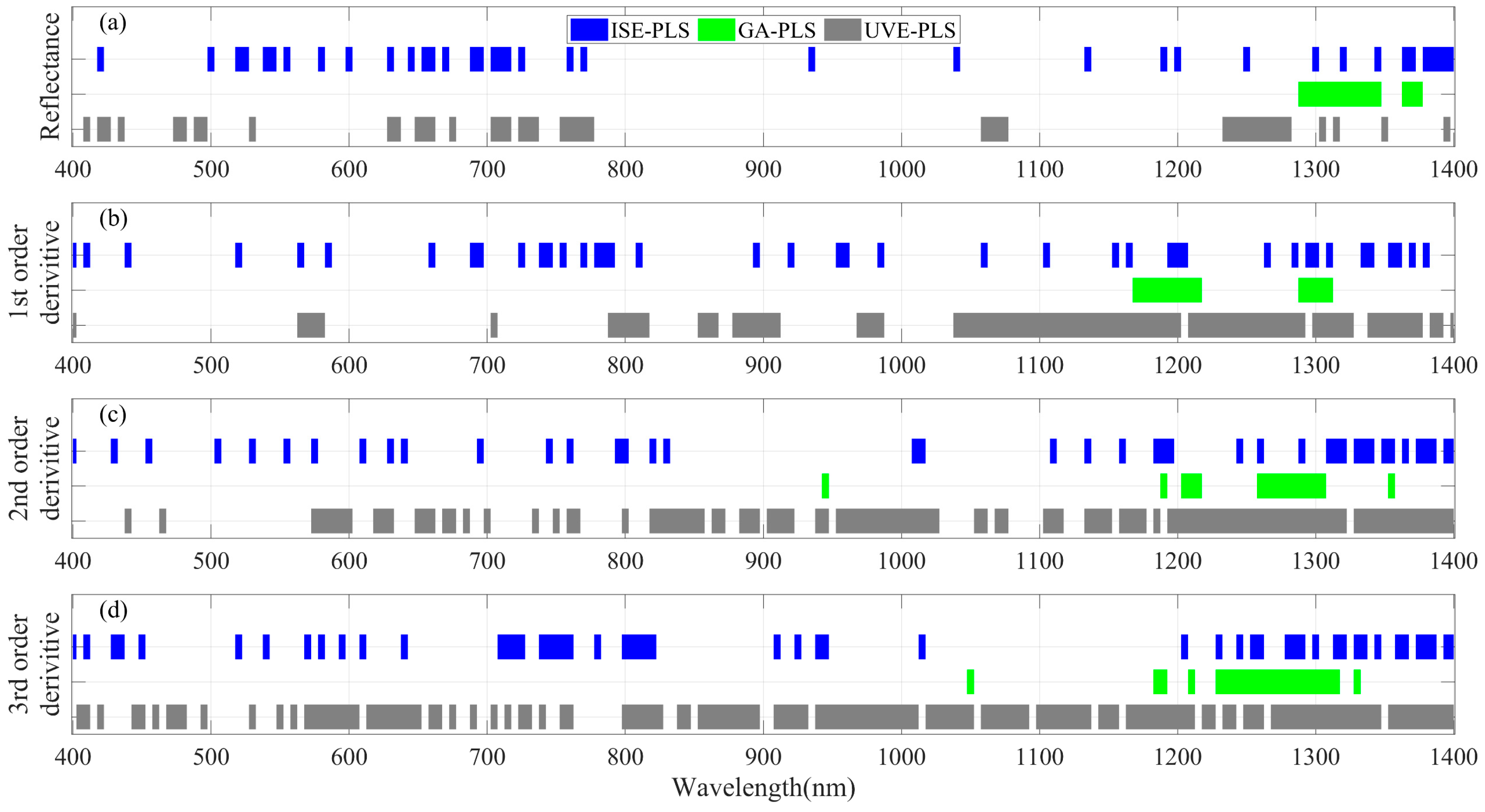
Furthermore, we have also attempted to build PLSR models based on the spectra from 400 to 1400 nm to estimate the LNC. Although nitrogen-based constituents (proteins) do not absorb radiation within 400–1400 nm (the specific absorption coefficients of proteins were zero in the PROSPECT-PRO model), the spectra within 400–1400 nm were unexpectedly used for LNC estimation using PLSR models (Figure 5). Most of the bands involved in the ISE-PLS regression models were found to be distributed within 400–800 nm and 1200–1400 nm, while the bands in the spectral region from 400 to 1400 nm were uniformly selected with the UVE band-selection method. Again, in comparison, much fewer bands were involved in GA-PLS regression models. Furthermore, the bands around 1300 nm were consistently identified as the most important bands for all four spectral forms (reflectance and derivatives) in GA-PLS regression models.
The statistical performance is shown in Table 3. The PLSR models based on the spectra within 400–1400 nm were inferior in capturing the variation in LNC compared with other wavelength-domain-trained PLSR models. Even though the FB-PLS and ISE-PLS regression models performed well for the simulation dataset, they exhibited poor performances with the field-measured validation datasets. The GA-PLS regression models again used the minimum number of bands. The AICc values of the GA-PLS and UVE-PLS regression models were smaller than those of the FB-PLS and ISE-PLS regression models, indicating better GoFs for the GA-PLS and UVE-PLS regression models.

3.4. PLSR Models Developed from Field Datasets Directly

We further developed PLSR models solely from field-measured datasets, as carried out by most previous studies, to investigate the performances of different methods to retrieve LNC from hyperspectral data within different spectral regions (400–2500 nm, 1400–2500 nm, and 400–1400 nm). We used 80 percent of all leaf samples (530 out of 662) randomly selected as calibration datasets for modeling, and the remaining 20 percent of leaf samples (132) for validation. A t-test was carried out on calibration and validation subsets to confirm that the two subsets covered the whole range of values for LNC appropriately and consistently.
Satisfied PLSR models were achieved, irrespective of the wavelength domains used (400–2500 nm, 1400–2500 nm, and 400–1400 nm). Furthermore, all PLSR models based on the original reflectance and the 1st-order derivative spectra performed well (both R2c and R2v values were around 0.80) to trace the variation in LNC; no statistical difference can be distinguished (Table 4).
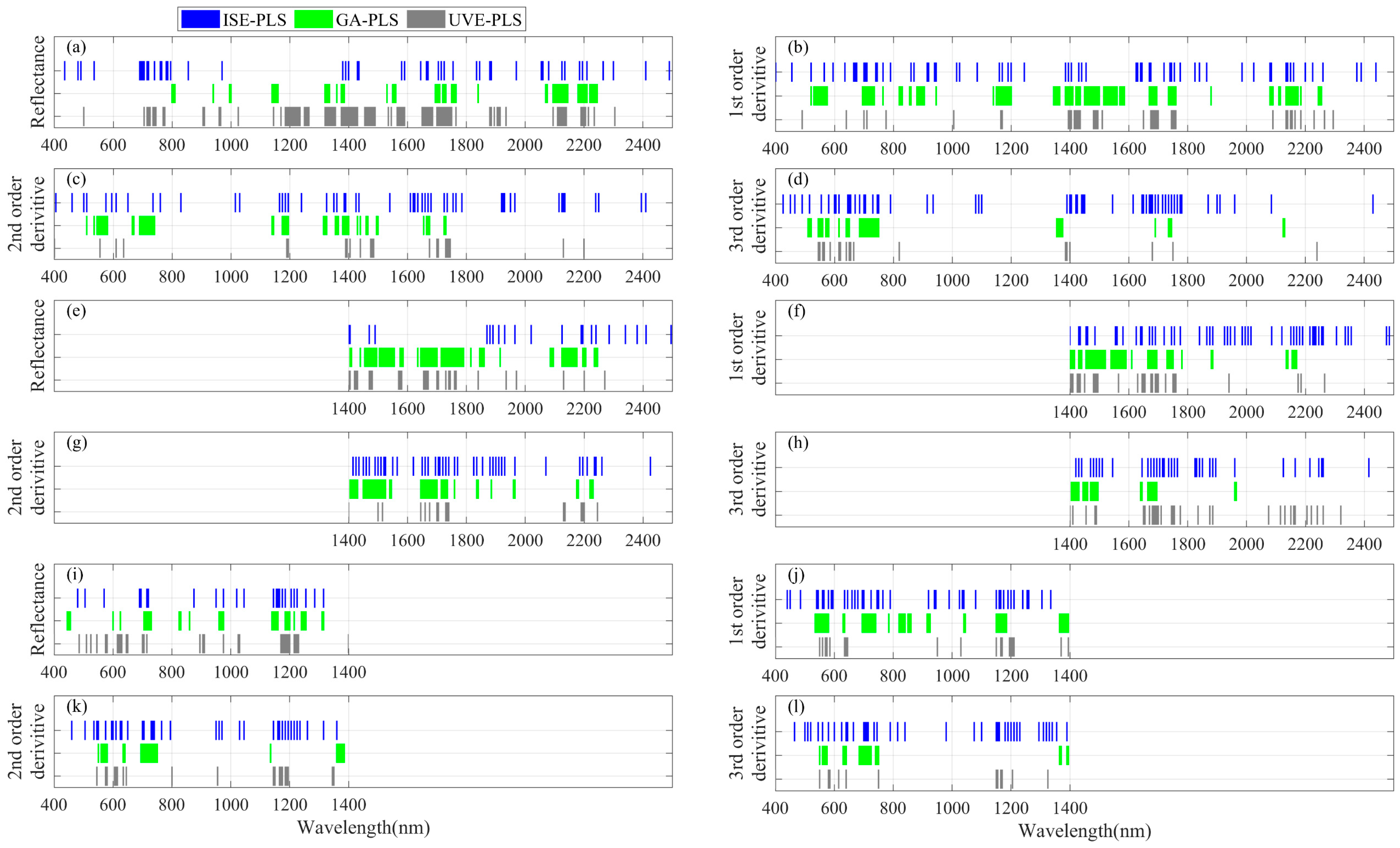
The informative bands (for each spectral domain) selected for ISE-PLS, GA-PLS, and UVE-PLS regression models are illustrated in Figure 6. Again, the bands within 1600–1800 nm were identified as the most important bands for LNC estimation in field-measured datasets with PLSR models when using the spectral regions of 400–2500 nm or 1400–2500 nm. In addition, the bands within 1400–1600 nm and around 2200 nm were also important for LNC estimation in field-measured datasets with PLSR models. In comparison, the bands around 1200 nm, 1400 nm, and 600–800 nm were selected as the most important bands when the spectral domain was limited to 400–1400 nm for PLSR models.

4. Discussion

4.1. Informative Band Selection—A Necessary Step for PLSR Models

PLSR modeling is a powerful statistical technique for correlating datasets (such as hyperspectral data) and has been widely used in the field of plant-trait estimation [1,56,65,66]. Unfortunately, most proposed PLSR models lack robustness for general applications [1,24,25,26]. This also applies to estimate the variations in the plant nitrogen status [1,4,5,14,16,35,36,37,38,39]. Despite many PLSR models having been proposed, most of them are without specific concerns for informative band selection. For example, Serbin et al. (2014) proposed a PLSR model using all bands within 1500–2400 nm for the foliar nitrogen concentration of temperate and boreal tree species estimation with an R2 value of 0.97 [2]. Using all bands within 350–1800 nm, Yao et al. (2015) built PLSR models for wheat LNC estimation based on the original and first derivative spectra [38]. Furthermore, Ely et al. (2019) demonstrated that the PLSR models with leaf reflectance (all bands within 500–2400 nm) of eight crop species (dataset A in this study) achieved high predictive power for LNC (R2 = 0.86) [16]. Dataset B used in this study, which was originally provided by Burnett et al. (2021), successfully predicted LNC with an R2 value of 0.87 [14] by the usage of full-spectrum (500–2400 nm) leaf reflectance data. In addition, the PLSR with leaf reflectance from 400 nm to 2200 nm was able to capture the seasonal variability in LNC in two temperate deciduous forests (R2 = 0.63) [4], while the PLSR model proposed by Wan et al. (2022) with leaf reflectance at 550–2300 nm achieved a satisfactory estimation of LNC with the R2 of 0.94 across different plant species [1]. These PLSR models using full bands always exhibited high R2 values in leaf traits retrieved from hyperspectral data but very possibly underwent overfitting, which seriously limits their transferability.
Alternatively, Tahmasbian et al. (2017) demonstrated that the PLSR model developed using the most important wavelengths (selected using regression coefficients from full band PLSR analysis) instead of all bands within 400–1700 nm was reliable (R2 = 0.64 for validation dataset) for the prediction of LNC in new forest leaf litterfall samples [39]. In this study, we combined a large simulation dataset with two public datasets from Ely et al. (2019) and Burnett et al. (2021) to generate PLSR models with a limited number of bands for LNC estimation and to verify the performance of calibrated PLSR models. The FB-PLS and ISE-PLS regression models calibrated from the training dataset (10,000 leaf samples simulated with PROSPECT-PRO model) failed to trace the variation in LNC in validation datasets. In comparison, the GA-PLS and UVE-PLS regression models with selected bands achieved satisfactory estimations of LNC even for validation datasets; their GoFs (evaluated with AICc) were dramatically improved as well. Thus, the PLSR models combining appropriate band-selection methods could closely trace LNC in the meantime with a low risk of overfitting.
The derivative technique is commonly used in deriving biophysical and biochemical parameters, as it holds the advantage of reducing noises and minimizing linear functions [40]. However, in this study, the PLSR models based on derivative spectra did not show notable improvement compared to those reflectance-based models. For example, the PLSR models based on the first-order derivative canopy spectra (R2 values for calibration and validation datasets were 0.91 and 0.85) and the original canopy spectra (R2 values were 0.82 and 0.81) demonstrated similar estimation accuracy for winter wheat LNC [38]. The PLSR model based on the first derivative performed even worse for estimating corn LNC than the reflectance-based model (R2 = 0.54 versus 0.59) [67]. Additionally, previous research on the estimation of total nitrogen in ground litterfall samples of a natural forest from hyperspectral images in the spectral range of 400–1700 nm also demonstrated that the reflectance-based PLSR model (R2 = 0.61) was more effective than the first-derivative-based PLSR model (R2 = 0.59) [39]. Our results were consistent with these reported studies, although out of expectations, confirming that derivative analysis is no longer a critical step when estimating LNC with a PLSR model. This also implies that PLSR analysis holds comparable abilities to reduce noises and minimize linear functions as well.
In addition, it has been reported that the accuracy of GA-PLS regression models for plant nitrogen content estimation could be improved using a combination of narrow-band reflectance data with spectral derivatives [68]. The original reflectance and its derivatives (the 1st, 2nd, and 3rd orders) within 400–2500 nm in the 5-nm resolution were combined together to form the composite spectral features (421 × 4 = 1684 variables in total). The results showed that all PLS regression models based on the composite spectral features were more effective to estimate LNC (R2 values were greater than 0.97 for the simulation dataset, dataset A and dataset B). Only the GA-PLS regression model clearly captured the sensitive bands (within 1600–1800 nm and around 2200 nm) for LNC estimation (Figure 7). The high accuracy of these PLS regression models suggests a promising scheme to accurately retrieve LNC from hyperspectral data but needs more investigations on overfitting [31].

4.2. Informative Bands Selected for PLSR Models—Evidence from the PROSPECT-PRO Radiative Transfer Model

The simulation dataset used in this study provides an ideal resource for assessing the informative band-selection methods since all wavelengths are with known physical bases. According to the specific absorption coefficient of nitrogen-based constituents defined in the PROSPECT-PRO model [3], the nitrogen-based constituents only absorb radiation within 1400–2500 nm (Figure 8a).
Astonishingly, only GA-PLS regression models captured the majority of bands inside this spectral region, with close agreements between the known spectral absorption features and the significant wavelengths selected by the GA for PLSR models, especially those absorption features within 1400–2500 nm [2]. Furthermore, the results also indicate that the most important bands involved in GA-PLS regression models for LNC estimation were those within 1600–1800 nm rather than the bands within 1800–2500 nm. A possible explanation for this is that the specific absorption coefficient of nitrogen-based constituents (KNBC, cm2 g−1) exhibited relatively low values within this spectral region (1600–1800 nm) if compared to those values within 1800–2500 nm, based on our previous finding that the relative absorptions of leaf biochemical contents were important to identify the informative bands for leaf biochemical-content estimation from hyperspectral data [26].
We have further explicitly investigated the relationships between the specific absorption coefficient of nitrogen-based constituents and other important leaf biochemical parameters in this spectral region (Figure 8b). Two main peaks (around 1700 nm and 2200 nm) were found for the relative absorption of nitrogen-based constituents to water (KNBC/Kw). The KNBC/Kw values within 1600–1800 nm were greater than 0.70 and were identified as the most important spectral region for LNC estimation with GA-PLS regression models. The relative absorption of nitrogen-based constituents to carbon-based constituents (KNBC/KCBC) was also high around 1700, 1900, and 2200 nm. However, the reflectance values within 1800–2500 nm (Figure 2) were lower than the values within 1600–1800 nm due to the strong absorption of water and leaf dry matter [8,69]. Low leaf nitrogen- and carbon-based constituents would be sufficient to saturate absorption in the spectral region; the peaks of KNBC/Kw and KNBC/KCBC around 1900 nm and 2200 nm were thus not identified as the informative spectral region for LNC estimation.
On the other hand, our results of PLSR models developed using the simulated 400–1400 nm spectra also suggested that the variation in LNC in the simulation dataset could be captured with PLSR models (especially with FB-PLS and ISE-PLS regression models) with this spectral region. Unfortunately, such PLSR models are not supported by physical mechanisms in the term. We attribute such a good performance of the PLSR model using the spectral information within 400–1400 nm to their high correlations with the bands beyond 1400 nm. In three individual datasets used in this study, the reflectance within 1600–1800 nm was highly correlated with those within 800–1400 nm (Figure 9).
Consequently, we conclude that the GA is capable of selecting informative bands with a solid physical basis for the PLSR model and should be applied for retrieving LNC from leaf spectral data. However, we noted that the developed GA-PLS models from the simulation dataset had relatively low accuracies when validated using field-measured datasets. This may be attributed to the fact that no nitrogen absorptance was set for the wavelength domain of 800–1400 nm of the simulation data when generated from the PROSPECT-PRO model. However, the majority of nitrogen is attributed to both proteins (absorbing radiation within 1400–2500 nm) and chlorophylls (absorbing radiation within 400–780 nm) stored in leaf cells [1]. As the LNC values in the simulation dataset were calculated from the nitrogen-based constituents using the suggested nitrogen-to-crude protein conversion factor of 4.43 [3], the nitrogen constituents in chlorophylls were lost. This should be the primary reason for the relative low accuracies of the GA-PLS regression model for LNC retrieval in validation datasets. The relationship between LNC and chlorophylls should also be taken into account in the future for generating more proper simulation data.

5. Conclusions

Our results demonstrate that the GoFs of PLSR models to estimate LNC could be greatly improved by combining appropriate band-selection methods instead of using full bands for PLSR. However, spectral transformations did not help in improving the performance of PLSR models and are therefore no longer the critical step of spectral preprocessing. Only the GA-PLS and UVE-PLS regression models calibrated from the simulation dataset were capable of retrieving LNC in the other two independent field-measured datasets. In particular, the genetic algorithm was more effective to capture the informative bands with solid physical bases. However, the applications of band selection methods in the PLSR models should be approached with caution since not all the bands selected have solid physical bases. These findings shall provide advanced information for the nondestructive tracking of plant nitrogen status from reflected information.

Author Contributions

Conceptualization, Q.W.; methodology, J.J.; validation, M.W.; data curation, G.S.; writing—original draft preparation, J.J.; writing—review and editing, Q.W., J.J., M.W. and G.S.; funding acquisition, J.J. All authors have read and agreed to the published version of the manuscript.

Funding

This research was supported by Zhejiang Provincial Natural Science Foundation (No. LQ19C160005) and the National Natural Science Foundation of China (No. 41901368) to Jia Jin.

Data Availability Statement

Not applicable.

Acknowledgments

We thank the Terrestrial Ecosystem Science and Technology (TEST) group at Brookhaven National Laboratory and Ecological Spectral Information System (EcoSIS) for the public datasets. We are also grateful to the public LOPEX database.

Conflicts of Interest

The authors declare no conflict of interest.

References

  1. Wan, L.; Zhou, W.; He, Y.; Wanger, T.C.; Cen, H. Combining transfer learning and hyperspectral reflectance analysis to assess leaf nitrogen concentration across different plant species datasets. Remote Sens. Environ. 2022, 269, 112826. [Google Scholar] [CrossRef]
  2. Serbin, S.P.; Singh, A.; McNeil, B.E.; Kingdon, C.C.; Townsend, P.A. Spectroscopic determination of leaf morphological and biochemical traits for northern temperate and boreal tree species. Ecol. Appl. 2014, 24, 1651–1669. [Google Scholar] [CrossRef] [PubMed] [Green Version]
  3. Féret, J.-B.; Berger, K.; de Boissieu, F.; Malenovský, Z. PROSPECT-PRO for estimating content of nitrogen-containing leaf proteins and other carbon-based constituents. Remote Sens. Environ. 2021, 252, 112173. [Google Scholar] [CrossRef]
  4. Yang, X.; Tang, J.; Mustard, J.F.; Wu, J.; Zhao, K.; Serbin, S.; Lee, J.-E. Seasonal variability of multiple leaf traits captured by leaf spectroscopy at two temperate deciduous forests. Remote Sens. Environ. 2016, 179, 1–12. [Google Scholar] [CrossRef] [Green Version]
  5. Chavana-Bryant, C.; Malhi, Y.; Anastasiou, A.; Enquist, B.J.; Cosio, E.G.; Keenan, T.F.; Gerard, F.F. Leaf age effects on the spectral predictability of leaf traits in Amazonian canopy trees. Sci. Total Environ. 2019, 666, 1301–1315. [Google Scholar] [CrossRef] [Green Version]
  6. Zhang, Y.; Migliavacca, M.; Penuelas, J.; Ju, W. Advances in hyperspectral remote sensing of vegetation traits and functions. Remote Sens. Environ. 2021, 252, 112121. [Google Scholar] [CrossRef]
  7. Gamon, J.A.; Somers, B.; Malenovský, Z.; Middleton, E.M.; Rascher, U.; Schaepman, M.E. Assessing Vegetation Function with Imaging Spectroscopy. Surv. Geophys. 2019, 40, 489–513. [Google Scholar] [CrossRef] [Green Version]
  8. Jin, J.; Wang, Q. Hyperspectral indices developed from the low order fractional derivative spectra can capture leaf dry matter content across a variety of species better. Agric. For. Meteorol. 2022, 322, 109007. [Google Scholar] [CrossRef]
  9. Main, R.; Cho, M.A.; Mathieu, R.; O’Kennedy, M.M.; Ramoelo, A.; Koch, S. An investigation into robust spectral indices for leaf chlorophyll estimation. ISPRS-J. Photogramm. Remote Sens. 2011, 66, 751–761. [Google Scholar] [CrossRef]
  10. Féret, J.B.; Gitelson, A.A.; Noble, S.D.; Jacquemoud, S. PROSPECT-D: Towards modeling leaf optical properties through a complete lifecycle. Remote Sens. Environ. 2017, 193, 204–215. [Google Scholar] [CrossRef]
  11. Ali, A.M.; Darvishzadeh, R.; Skidmore, A.K.; Duren, I.v.; Heiden, U.; Heurich, M. Estimating leaf functional traits by inversion of PROSPECT: Assessing leaf dry matter content and specific leaf area in mixed mountainous forest. Int. J. Appl. Earth Obs. Geoinf. 2016, 45, 66–76. [Google Scholar] [CrossRef] [Green Version]
  12. Rubo, S.; Zinkernagel, J. Exploring hyperspectral reflectance indices for the estimation of water and nitrogen status of spinach. Biosys. Eng. 2022, 214, 58–71. [Google Scholar] [CrossRef]
  13. He, L.; Liu, M.-R.; Guo, Y.-L.; Wei, Y.-K.; Zhang, H.-Y.; Song, X.; Feng, W.; Guo, T.-C. Angular effect of algorithms for monitoring leaf nitrogen concentration of wheat using multi-angle remote sensing data. Comput. Electron. Agric. 2022, 195, 106815. [Google Scholar] [CrossRef]
  14. Burnett, A.C.; Serbin, S.P.; Davidson, K.J.; Ely, K.S.; Rogers, A. Detection of the metabolic response to drought stress using hyperspectral reflectance. J. Exp. Bot. 2021, 72, 6474–6489. [Google Scholar] [CrossRef] [PubMed]
  15. Berger, K.; Verrelst, J.; Féret, J.-B.; Wang, Z.; Wocher, M.; Strathmann, M.; Danner, M.; Mauser, W.; Hank, T. Crop nitrogen monitoring: Recent progress and principal developments in the context of imaging spectroscopy missions. Remote Sens. Environ. 2020, 242, 111758. [Google Scholar] [CrossRef] [PubMed]
  16. Ely, K.S.; Burnett, A.C.; Lieberman-Cribbin, W.; Serbin, S.P.; Rogers, A. Spectroscopy can predict key leaf traits associated with source-sink balance and carbon-nitrogen status. J. Exp. Bot. 2019, 70, 1789–1799. [Google Scholar] [CrossRef] [Green Version]
  17. Kawamura, K.; Watanabe, N.; Sakanoue, S.; Lee, H.J.; Inoue, Y.; Odagawa, S. Testing genetic algorithm as a tool to select relevant wavebands from field hyperspectral data for estimating pasture mass and quality in a mixed sown pasture using partial least squares regression. Grassl. Sci. 2010, 56, 205–216. [Google Scholar] [CrossRef]
  18. Huang, Z.; Turner, B.J.; Dury, S.J.; Wallis, I.R.; Foley, W.J. Estimating foliage nitrogen concentration from HYMAP data using continuum removal analysis. Remote Sens. Environ. 2004, 93, 18–29. [Google Scholar] [CrossRef]
  19. Thenkabail, P.S.; Lyon, J.G.; Huete, A. Hyperspectral Remote Sensing of Vegetation; CRC Press: Boca Raton, FL, USA, 2012. [Google Scholar]
  20. Hansen, P.M.; Schjoerring, J.K. Reflectance measurement of canopy biomass and nitrogen status in wheat crops using normalized difference vegetation indices and partial least squares regression. Remote Sens. Environ. 2003, 86, 542–553. [Google Scholar] [CrossRef]
  21. Yi, Q.; Jiapaer, G.; Chen, J.; Bao, A.; Wang, F. Different units of measurement of carotenoids estimation in cotton using hyperspectral indices and partial least square regression. ISPRS-J. Photogramm. Remote Sens. 2014, 91, 72–84. [Google Scholar] [CrossRef]
  22. Dorigo, W.A.; Zurita-Milla, R.; de Wit, A.J.W.; Brazile, J.; Singh, R.; Schaepman, M.E. A review on reflective remote sensing and data assimilation techniques for enhanced agroecosystem modeling. Int. J. Appl. Earth Obs. Geoinf. 2007, 9, 165–193. [Google Scholar] [CrossRef]
  23. Asner, G.P.; Martin, R.E. Spectral and chemical analysis of tropical forests: Scaling from leaf to canopy levels. Remote Sens. Environ. 2008, 112, 3958–3970. [Google Scholar] [CrossRef]
  24. le Maire, G.; François, C.; Soudani, K.; Berveiller, D.; Pontailler, J.-Y.; Bréda, N.; Genet, H.; Davi, H.; Dufrêne, E. Calibration and validation of hyperspectral indices for the estimation of broadleaved forest leaf chlorophyll content, leaf mass per area, leaf area index and leaf canopy biomass. Remote Sens. Environ. 2008, 112, 3846–3864. [Google Scholar] [CrossRef]
  25. Féret, J.-B.; François, C.; Gitelson, A.; Asner, G.P.; Barry, K.M.; Panigada, C.; Richardson, A.D.; Jacquemoud, S. Optimizing spectral indices and chemometric analysis of leaf chemical properties using radiative transfer modeling. Remote Sens. Environ. 2011, 115, 2742–2750. [Google Scholar] [CrossRef] [Green Version]
  26. Jin, J.; Wang, Q. Informative bands used by efficient hyperspectral indices to predict leaf biochemical contents are determined by their relative absorptions. Int. J. Appl. Earth Obs. Geoinf. 2018, 73, 616–626. [Google Scholar] [CrossRef]
  27. Wu, Q.; Wang, J.; Wang, C.; Xu, T. Study on the optimal algorithm prediction of corn leaf component information based on hyperspectral imaging. Infrared Phys. Technol. 2016, 78, 66–71. [Google Scholar] [CrossRef]
  28. Chen, H.; Chen, T.; Zhang, Z.; Liu, G. Variable Selection Using Adaptive Band Clustering and Physarum Network. Algorithms 2017, 10, 73. [Google Scholar] [CrossRef] [Green Version]
  29. Wang, Z.; Kawamura, K.; Sakuno, Y.; Fan, X.; Gong, Z.; Lim, J. Retrieval of Chlorophyll-a and Total Suspended Solids Using Iterative Stepwise Elimination Partial Least Squares (ISE-PLS) Regression Based on Field Hyperspectral Measurements in Irrigation Ponds in Higashihiroshima, Japan. Remote Sens. 2017, 9, 264. [Google Scholar] [CrossRef] [Green Version]
  30. Mehmood, T.; Liland, K.H.; Snipen, L.; Sæbø, S. A review of variable selection methods in Partial Least Squares Regression. Chemom. Intell. Lab. Syst. 2012, 118, 62–69. [Google Scholar] [CrossRef]
  31. Jin, J.; Wang, Q. Selection of informative spectral bands for PLS models to estimate foliar chlorophyll content using hyperspectral reflectance. IEEE Trans. Geosci. Remote Sens. 2019, 57, 3064–3072. [Google Scholar] [CrossRef]
  32. Centner, V.; Massart, D.-L.; de Noord, O.E.; de Jong, S.; Vandeginste, B.M.; Sterna, C. Elimination of Uninformative Variables for Multivariate Calibration. Anal. Chem. 1996, 68, 3851–3858. [Google Scholar] [CrossRef] [PubMed]
  33. Cai, W.; Li, Y.; Shao, X. A variable selection method based on uninformative variable elimination for multivariate calibration of near-infrared spectra. Chemom. Intell. Lab. Syst. 2008, 90, 188–194. [Google Scholar] [CrossRef]
  34. Leardi, R.; Boggia, R.; Terrile, M. Genetic algorithms as a strategy for feature selection. J. Chemom. 1992, 6, 267–281. [Google Scholar] [CrossRef]
  35. Burnett, A.C.; Serbin, S.P.; Rogers, A. Source:sink imbalance detected with leaf- and canopy-level spectroscopy in a field-grown crop. Plant Cell Environ. 2021, 44, 2466–2479. [Google Scholar] [CrossRef]
  36. Chavana-Bryant, C.; Malhi, Y.; Wu, J.; Asner, G.P.; Anastasiou, A.; Enquist, B.J.; Cosio Caravasi, E.G.; Doughty, C.E.; Saleska, S.R.; Martin, R.E.; et al. Leaf aging of Amazonian canopy trees as revealed by spectral and physiochemical measurements. New Phytol. 2017, 214, 1049–1063. [Google Scholar] [CrossRef] [PubMed] [Green Version]
  37. Li, Z.; Nie, C.; Wei, C.; Xu, X.; Song, X.; Wang, J. Comparison of Four Chemometric Techniques for Estimating Leaf Nitrogen Concentrations in Winter Wheat (Triticum Aestivum) Based on Hyperspectral Features. J. Appl. Spectrosc. 2016, 83, 240–247. [Google Scholar] [CrossRef]
  38. Yao, X.; Huang, Y.; Shang, G.; Zhou, C.; Cheng, T.; Tian, Y.; Cao, W.; Zhu, Y. Evaluation of Six Algorithms to Monitor Wheat Leaf Nitrogen Concentration. Remote Sens. 2015, 7, 14939–14966. [Google Scholar] [CrossRef] [Green Version]
  39. Tahmasbian, I.; Xu, Z.; Abdullah, K.; Zhou, J.; Esmaeilani, R.; Nguyen, T.T.N.; Hosseini Bai, S. The potential of hyperspectral images and partial least square regression for predicting total carbon, total nitrogen and their isotope composition in forest litterfall samples. J. Soils Sed. 2017, 17, 2091–2103. [Google Scholar] [CrossRef]
  40. Wang, Q.; Jin, J.; Sonobe, R.; Chen, J.M. Derivative hyperspectral vegetation indices in characterizing forest biophysical and biochemical quantities. In Hyperspectral Indices and Image Classifications for Agriculture and Vegetation; Thenkabail, P.S., Lyon, J.G., Huete, A., Eds.; CRC Press: Boca Raton, FL, USA, 2018; pp. 27–63. [Google Scholar]
  41. Huguenin, R.L.; Jones, J.L. Intelligent information extraction from reflectance spectra: Absorption band positions. J. Geophys. Res. Solid Earth 1986, 91, 9585–9598. [Google Scholar] [CrossRef]
  42. Becker, B.L.; Lusch, D.P.; Qi, J. Identifying optimal spectral bands from in situ measurements of Great Lakes coastal wetlands using second-derivative analysis. Remote Sens. Environ. 2005, 97, 238–248. [Google Scholar] [CrossRef]
  43. Tsai, F.; Philpot, W. Derivative Analysis of Hyperspectral Data. Remote Sens. Environ. 1998, 66, 41–51. [Google Scholar] [CrossRef]
  44. Demetriades-Shah, T.H.; Steven, M.D.; Clark, J.A. High resolution derivative spectra in remote sensing. Remote Sens. Environ. 1990, 33, 55–64. [Google Scholar] [CrossRef]
  45. Abulaiti, Y.; Sawut, M.; Maimaitiaili, B.; Chunyue, M. A possible fractional order derivative and optimized spectral indices for assessing total nitrogen content in cotton. Comput. Electron. Agric. 2020, 171, 105275. [Google Scholar] [CrossRef]
  46. Jacquemoud, S.; Baret, F. PROSPECT: A model of leaf optical properties spectra. Remote Sens. Environ. 1990, 34, 75–91. [Google Scholar] [CrossRef]
  47. Hosgood, B.; Jacquemoud, S.; Andreoli, G.; Verdebout, J.; Pedrini, G.; Schmuck, G. Leaf Optical Properties Experiment 93 (LOPEX93); European Commission—Joint Research Centre EUR 16095 EN: Ispra, Italy, 1994; p. 20. [Google Scholar]
  48. Stein, M. Large Sample Properties of Simulations Using Latin Hypercube Sampling. Technometrics 1987, 29, 143–151. [Google Scholar] [CrossRef]
  49. Ely, K.S.; Serbin, S.P.; Lieberman-Cribbin, W.; Rogers, A. Leaf Spectra, Structural and Biochemical Leaf Traits of Eight Crop Species. Ecological Spectral Information System (EcoSIS), 2018. Available online: http://ecosis.org (accessed on 2 September 2021). [CrossRef]
  50. Burnett, A.C.; Serbin, S.P.; Davidson, K.J.; Ely, K.S.; Rogers, A. Hyperspectral Leaf Reflectance, Biochemistry, and Physiology of Droughted and Watered Crops. Ecological Spectral Information System (EcoSIS), 2020. Available online: http://ecosis.org (accessed on 2 September 2021). [CrossRef]
  51. Vaiphasa, C. Consideration of smoothing techniques for hyperspectral remote sensing. ISPRS-J. Photogramm. Remote Sens. 2006, 60, 91–99. [Google Scholar] [CrossRef]
  52. Marang, I.J.; Filippi, P.; Weaver, T.B.; Evans, B.J.; Whelan, B.M.; Bishop, T.F.A.; Murad, M.O.F.; Al-Shammari, D.; Roth, G. Machine Learning Optimised Hyperspectral Remote Sensing Retrieves Cotton Nitrogen Status. Remote Sens. 2021, 13, 1428. [Google Scholar] [CrossRef]
  53. Boggia, R.; Forina, M.; Fossa, P.; Mosti, L. Chemometric Study and Validation Strategies in the Structure-Activity Relationships of New Cardiotonic Agents. Quant. Struct.-Act. Relat. 1997, 16, 201–213. [Google Scholar] [CrossRef]
  54. Leardi, R. Application of genetic algorithm–PLS for feature selection in spectral data sets. J. Chemom. 2000, 14, 643–655. [Google Scholar] [CrossRef]
  55. Leardi, R.; Lupiáñez González, A. Genetic algorithms applied to feature selection in PLS regression: How and when to use them. Chemom. Intell. Lab. Syst. 1998, 41, 195–207. [Google Scholar] [CrossRef]
  56. Burnett, A.C.; Anderson, J.; Davidson, K.J.; Ely, K.S.; Lamour, J.; Li, Q.; Morrison, B.D.; Yang, D.; Rogers, A.; Serbin, S.P. A best-practice guide to predicting plant traits from leaf-level hyperspectral data using partial least squares regression. J. Exp. Bot. 2021, 72, 6175–6189. [Google Scholar] [CrossRef] [PubMed]
  57. Fushiki, T. Estimation of prediction error by using K-fold cross-validation. Stat. Comput. 2011, 21, 137–146. [Google Scholar] [CrossRef]
  58. Deepak, M.; Keski-Saari, S.; Fauch, L.; Granlund, L.; Oksanen, E.; Keinänen, M. Leaf Canopy Layers Affect Spectral Reflectance in Silver Birch. Remote Sens. 2019, 11, 2884. [Google Scholar] [CrossRef] [Green Version]
  59. Mishra, P.; Asaari, M.S.M.; Herrero-Langreo, A.; Lohumi, S.; Diezma, B.; Scheunders, P. Close range hyperspectral imaging of plants: A review. Biosys. Eng. 2017, 164, 49–67. [Google Scholar] [CrossRef]
  60. McQuarrie, A.D.R.; Tsai, C.-L. Regression and Time Series Model Selection; World Scientific: Singapore, 1998. [Google Scholar]
  61. Hurvich, C.M.; Tsai, C.-L. Regression and Time Series Model Selection in Small Samples. Biometrika 1989, 76, 297–307. [Google Scholar] [CrossRef]
  62. Akaike, H. A new look at the statistical model identification. IEEE Trans. Autom. Control 1974, 19, 716–723. [Google Scholar] [CrossRef]
  63. Burnham, K.P.; Anderson, D.R. Multimodel Inference:Understanding AIC and BIC in Model Selection. Sociol. Methods Res. 2004, 33, 261–304. [Google Scholar] [CrossRef]
  64. Bozdogan, H. Model selection and Akaike’s Information Criterion (AIC): The general theory and its analytical extensions. Psychometrika 1987, 52, 345–370. [Google Scholar] [CrossRef]
  65. Verma, B.; Prasad, R.; Srivastava, P.K.; Yadav, S.A.; Singh, P.; Singh, R.K. Investigation of optimal vegetation indices for retrieval of leaf chlorophyll and leaf area index using enhanced learning algorithms. Comput. Electron. Agric. 2022, 192, 106581. [Google Scholar] [CrossRef]
  66. Jin, J.; Wang, Q. Evaluation of Informative Bands Used in Different PLS Regressions for Estimating Leaf Biochemical Contents from Hyperspectral Reflectance. Remote Sens. 2019, 11, 197. [Google Scholar] [CrossRef] [Green Version]
  67. Fan, L.; Zhao, J.; Xu, X.; Liang, D.; Yang, G.; Feng, H.; Yang, H.; Wang, Y.; Chen, G.; Wei, P. Hyperspectral-based Estimation of Leaf Nitrogen Content in Corn Using Optimal Selection of Multiple Spectral Variables. Sensors 2019, 19, 2898. [Google Scholar] [CrossRef] [PubMed] [Green Version]
  68. Thorp, K.R.; Wang, G.; Bronson, K.F.; Badaruddin, M.; Mon, J. Hyperspectral data mining to identify relevant canopy spectral features for estimating durum wheat growth, nitrogen status, and grain yield. Comput. Electron. Agric. 2017, 136, 1–12. [Google Scholar] [CrossRef] [Green Version]
  69. Yang, B.; He, Y.; Chen, W. A simple method for estimation of leaf dry matter content in fresh leaves using leaf scattering albedo. Glob. Ecol. Conserv. 2020, 23, e01201. [Google Scholar] [CrossRef]
Figure 1. Properties of LNC in different datasets. Dataset A&B is a composite of all field-measured leaf samples in both dataset A and dataset B. The statistical meanings in the diagram are illustrated in the left panel.
Remotesensing 14 05204 g001
Figure 2. Leaf spectra (raw values in 1 nm resolution) in different datasets ((a): simulation dataset, (b): dataset A, (c): dataset B). Each gray line represents the reflectance of one leaf sample. The dashed line in each panel represents the averaged value at each wavelength for all leaf samples.
Remotesensing 14 05204 g002
Figure 3. Distribution of bands selected with different band-selection methods for LNC estimation from spectra within 1400–2500 nm. (a) Reflectance. (b) The 1st-order derivative spectra. (c) The 2nd-order derivative. (d) The 3rd-order derivative. The locations of the color blocks in the Wavelength-axis represent the bands involved in different PLS (blue for ISE-PLS, green for GA-PLS, and grey for UVE-PLS) regression models.
Remotesensing 14 05204 g003
Figure 4. Distribution of bands selected with different band-selection methods for LNC estimation from spectra within 400–2500 nm. (a) Reflectance. (b) The 1st-order derivative spectra. (c) The 2nd-order derivative. (d) The 3rd-order derivative. The locations of the color blocks in the Wavelength-axis represent the bands involved in different PLS (blue for ISE-PLS, green for GA-PLS and grey for UVE-PLS) regression models.
Remotesensing 14 05204 g004
Figure 5. Distribution of bands selected with different band-selection methods for LNC estimation from spectra within 400–1400 nm. (a) Reflectance. (b) The 1st-order derivative spectra. (c) The 2nd-order derivative. (d) The 3rd-order derivative. The locations of the color blocks in the Wavelength-axis represent the bands involved in different PLS (blue for ISE-PLS, green for GA-PLS and grey for UVE-PLS) regression models.
Remotesensing 14 05204 g005
Figure 6. Distribution of bands selected by different band-selection methods for LNC estimation from field-measured spectra at three different spectral domains: (ad), 400–2500 nm; (eh), 1400–2500 nm; (il), 400–1400 nm. The locations of the color blocks in the Wavelength-axis represent the bands involved in different PLS (blue for ISE-PLS, green for GA-PLS and grey for UVE-PLS) regression models.
Remotesensing 14 05204 g006
Figure 7. Distribution of bands selected with different band-selection methods for LNC estimation from combined spectra (reflectance, 1st, 2nd, and 3rd derivatives) within 400–2500 nm.
Remotesensing 14 05204 g007
Figure 8. Specific absorption coefficients: (a) Of dry matter, nitrogen-based constituents (proteins), and carbon-based constituents in radiative transfer model PROSPECT-PRO and relative absorption. (b) Of nitrogen-based constituents to water (KNBC/Kw) and nitrogen-based constituents to carbon-based constituents (KNBC/KCBC).
Remotesensing 14 05204 g008
Figure 9. The linear correlation coefficients between different spectral bands in three datasets: (a) Simulation dataset. (b) Dataset A. (c) Dataset B.
Remotesensing 14 05204 g009
Table 1. PLSR model performance in estimating LNC from spectra within 1400–2500 nm with different band-selection methods. The number of bands (N_bands) used in each PLSR model and the coefficient of determination values for the simulation dataset (R2m), dataset A (R2A), and dataset B (R2B) are shown in the table.
Spectral FormMethodN_BandsR2mR2AR2BAICc
Original reflectanceFB-PLS2211.00 0.00 0.02 2.60
ISE-PLS581.00 0.05 0.20 2.90
GA-PLS410.98 0.64 0.63 −2.44
UVE-PLS1750.99 0.75 0.71 −2.78
First-order derivativeFB-PLS2211.00 0.06 0.00 3.02
ISE-PLS921.00 0.04 0.01 3.07
GA-PLS190.97 0.39 0.40 −1.90
UVE-PLS1950.99 0.75 0.75 −2.99
Second-order derivativeFB-PLS2211.00 0.21 0.05 2.41
ISE-PLS1171.00 0.20 0.02 3.83
GA-PLS230.96 0.53 0.42 −1.93
UVE-PLS2010.99 0.68 0.72 −2.82
Third-order derivativeFB-PLS2211.00 0.15 0.02 4.47
ISE-PLS1261.00 0.06 0.02 4.43
GA-PLS620.98 0.51 0.51 −2.10
UVE-PLS1830.99 0.57 0.59 −2.40
Table 2. PLSR model performance in estimating LNC from spectra within 400–2500 nm with different band-selection methods. The number of bands (N_bands) used in each PLSR model and the coefficient of determination values for the simulation dataset (R2m), dataset A (R2A), and dataset B (R2B) are shown in the table.
Spectral FormMethodN_BandsR2mR2AR2BAICc
Original reflectanceFB-PLS4211.00 0.01 0.00 2.53
ISE-PLS780.99 0.00 0.00 2.27
GA-PLS240.98 0.35 0.55 −2.24
UVE-PLS3010.98 0.34 0.64 −2.30
First-order derivativeFB-PLS4211.00 0.04 0.20 −1.42
ISE-PLS1331.00 0.03 0.03 −0.22
GA-PLS290.99 0.53 0.51 −2.31
UVE-PLS3000.99 0.69 0.78 −3.05
Second-order derivativeFB-PLS4210.99 0.01 0.16 −0.24
ISE-PLS1351.00 0.17 0.02 1.14
GA-PLS510.99 0.59 0.55 −2.43
UVE-PLS2830.99 0.65 0.73 −2.77
Third-order derivativeFB-PLS4210.99 0.00 0.08 1.85
ISE-PLS1351.00 0.06 0.02 3.36
GA-PLS500.98 0.24 0.25 −1.72
UVE-PLS2590.99 0.49 0.63 −2.43
Table 3. PLSR model performance in estimating LNC from spectra within 400–1400 nm with different band-selection methods. The number of bands (N_bands) used in each PLSR model and the coefficient of determination values for the simulation dataset (R2m), dataset A (R2A), and dataset B (R2B) are shown in the table.
Spectral FormMethodN_BandsR2mR2AR2BAICc
Original reflectanceFB-PLS2010.43 0.04 0.21 3.81
ISE-PLS380.94 0.00 0.01 6.12
GA-PLS150.40 0.15 0.31 0.11
UVE-PLS440.42 0.40 0.66 0.02
First-order derivativeFB-PLS2010.51 0.06 0.05 5.68
ISE-PLS410.96 0.04 0.03 8.21
GA-PLS150.30 0.11 0.24 0.25
UVE-PLS930.43 0.69 0.71 0.01
Second-order derivativeFB-PLS2010.64 0.00 0.06 6.25
ISE-PLS420.96 0.09 0.01 7.86
GA-PLS160.29 0.09 0.28 0.24
UVE-PLS1140.42 0.52 0.73 0.02
Third-order derivativeFB-PLS2010.63 0.00 0.00 7.65
ISE-PLS530.92 0.01 0.02 6.04
GA-PLS230.30 0.01 0.16 0.25
UVE-PLS1450.42 0.49 0.71 0.03
Table 4. PLSR model performance in estimating LNC from spectra within different spectral regions (400–2500 nm, 1400–2500 nm, and 400–1400 nm) with different band selection methods. The number of bands (N_bands) used in each PLSR model and the coefficient of determination values for calibration subset (R2c) and validation subset (R2v) of field-measured datasets, dataset A (R2A) and dataset B (R2B), were shown in the table.
Spectral RegionSpectral FormMethodN_BandsR2cR2vR2AR2BAICc
400–2500 nmOriginal reflectanceFB-PLS4210.87 0.87 0.74 0.86 2.45
ISE-PLS490.88 0.86 0.81 0.87 −0.99
GA-PLS610.80 0.81 0.75 0.79 −0.47
UVE-PLS1100.87 0.89 0.75 0.88 −0.75
1st order derivativeFB-PLS4210.91 0.84 0.82 0.89 2.20
ISE-PLS640.91 0.84 0.81 0.89 −1.08
GA-PLS1160.85 0.87 0.72 0.85 −0.53
UVE-PLS420.81 0.84 0.74 0.80 −0.61
2nd order derivativeFB-PLS4210.90 0.78 0.71 0.87 2.45
ISE-PLS520.89 0.80 0.79 0.86 −0.93
GA-PLS530.78 0.77 0.58 0.78 −0.39
UVE-PLS220.65 0.68 0.63 0.63 −0.07
3rd order derivativeFB-PLS4210.86 0.70 0.60 0.83 2.73
ISE-PLS580.82 0.73 0.58 0.80 −0.46
GA-PLS390.72 0.76 0.40 0.75 −0.24
UVE-PLS180.62 0.69 0.43 0.64 −0.03
1400–2500 nmOriginal reflectanceFB-PLS2210.87 0.77 0.80 0.84 0.06
ISE-PLS210.81 0.76 0.76 0.78 −0.60
GA-PLS810.81 0.82 0.81 0.81 −0.46
UVE-PLS280.80 0.82 0.78 0.79 −0.61
1st order derivativeFB-PLS2210.89 0.74 0.81 0.84 0.07
ISE-PLS510.87 0.74 0.80 0.83 −0.74
GA-PLS540.80 0.82 0.78 0.78 −0.49
UVE-PLS290.74 0.77 0.60 0.75 −0.35
2nd order derivativeFB-PLS2210.85 0.70 0.82 0.79 0.28
ISE-PLS430.85 0.68 0.83 0.78 −0.53
GA-PLS520.73 0.75 0.70 0.72 −0.22
UVE-PLS170.57 0.62 0.58 0.54 0.12
3rd order derivativeFB-PLS2210.77 0.53 0.71 0.68 0.73
ISE-PLS360.81 0.68 0.77 0.76 −0.46
GA-PLS270.63 0.59 0.45 0.61 0.05
UVE-PLS320.56 0.58 0.42 0.54 0.20
400–1400 nmOriginal reflectanceFB-PLS2010.81 0.81 0.58 0.82 0.13
ISE-PLS240.81 0.78 0.58 0.81 −0.62
GA-PLS340.73 0.75 0.44 0.74 −0.29
UVE-PLS340.75 0.76 0.49 0.77 −0.36
1st order derivativeFB-PLS2010.85 0.79 0.65 0.83 0.02
ISE-PLS420.85 0.77 0.63 0.83 −0.70
GA-PLS510.72 0.75 0.49 0.73 −0.19
UVE-PLS200.68 0.72 0.63 0.68 −0.18
2nd order derivativeFB-PLS2010.83 0.73 0.52 0.82 0.16
ISE-PLS370.83 0.80 0.60 0.82 −0.66
GA-PLS270.69 0.71 0.37 0.73 −0.16
UVE-PLS200.74 0.77 0.57 0.75 −0.37
3rd order derivativeFB-PLS2010.81 0.73 0.44 0.80 0.26
ISE-PLS400.79 0.72 0.47 0.78 −0.42
GA-PLS240.66 0.72 0.44 0.69 −0.10
UVE-PLS130.54 0.60 0.42 0.53 0.17
Publisher’s Note: MDPI stays neutral with regard to jurisdictional claims in published maps and institutional affiliations.