Article

Random Matrix Theory-Based Reduced-Dimension Space-Time Adaptive Processing under Finite Training Samples

School of Electronic and Optical Engineering, Nanjing University of Science and Technology, Nanjing 210094, China
*
Author to whom correspondence should be addressed.
Remote Sens. 2022, 14(16), 3959; https://doi.org/10.3390/rs14163959
Submission received: 8 July 2022 / Revised: 6 August 2022 / Accepted: 12 August 2022 / Published: 15 August 2022
(This article belongs to the Special Issue Small or Moving Target Detection with Advanced Radar System)

Abstract

:
Space-time adaptive processing (STAP) is a fundamental topic in airborne radar applications due to its clutter suppression ability. Reduced-dimension (RD)-STAP can release the requirement of the number of training samples and reduce the computational load from traditional STAP, which attracts much attention. However, under the situation that training samples are severely deficient, RD-STAP will become poor like the traditional STAP. To enhance RD-STAP performance in such cases, this paper develops a novel RD-STAP algorithm using random matrix theory (RMT), RMT-RD-STAP. By minimizing the output clutter-plus-noise power, the estimate of the inversion of clutter plus noise covariance matrix (CNCM) can be obtained through optimally manipulating its eigenvalues, thus producing the optimal STAP weight vector. Specifically, the clutter-related eigenvalues are estimated according to the clutter-related sample eigenvalues via RMT, and the noise-related eigenvalue is optimally selected from the noise-related sample eigenvalues. It is found that RMT-RD-STAP significantly outperforms the RD-STAP algorithm when the RMB rule cannot be satisfied. Theoretical analyses and numerical results demonstrate the effectiveness and the performance advantages of the proposed RMT-RD-STAP algorithm.

1. Introduction

Space-time adaptive processing (STAP) was first proposed almost 50 years ago [1], and since then it has been actively investigated by the radar community due to its strong capability in suppressing clutter and enhancing target [2,3,4,5,6]. The optimal STAP can maximize the output signal-to-interference plus noise ratio (SINR) and provide reliable target detection. However, the optimal STAP involves an ideal clutter plus noise covariance matrix (CNCM), which generally cannot be attained and must be estimated with independent identical distributed (IID) training samples, called sample covariance matrix (SCM). Once the number of training samples for SCM is insufficient, STAP would severely suffer from performance deterioration. Particularly, the famous Reed, Mallet, and Brennan (RMB) rule [4] provides an explicit theoretical guide for the requirement on the number of training samples, i.e., to limit the SINR loss to 3 dB, the number of training samples must be not less than two times the system degrees of freedom (DoFs). However, in practice, the RMB rule is commonly hard to satisfy. In addition, the computational load in optimal STAP is extremely huge owing to high-dimensional matrix inversion. Therefore, the traditional STAP needs to be improved.
With the development of STAP, a great number of methods have been developed to confront the performance deterioration stemming from finite training samples. Sparsity-recovery (SR)-STAP [7,8,9,10] can greatly improve the SCM with only a few or even one training sample, however, the computational load involved in SR is unbearable. Knowledge-aided (KA)-STAP [11,12,13,14] uses the prior knowledge to improve SCM, i.e., covariance matrix and terrain data, but its performance will severely deteriorate once the prior knowledge deviates from the actual one. Recently, deep convolutional neural networks (CNNs) [15,16,17] have been used for STAP also with few training samples, but it usually needs a lot of sampling data as the training set for network learning, which is unavailable in many radar scenarios. Moreover, it is hard to obtain the ground truth in actual clutter scenarios, which is necessarily required as a label for supervised learning.
Reduced-dimension (RD)-STAP [18,19,20,21,22,23] is one of the most popular methods due to its fast convergence, simple structure, and a low requirement for training samples, which has been widely used in engineering applications. RD-STAP algorithms reduce the system DoFs through linear transformation on training samples to satisfy the RMB rule. Meanwhile, the lower system DoFs cause lower computational load, which significantly boosts real-time processing for airborne radar. In terms of different principles, several linear transformations have been constructed, such as the extended factored approach (EFA) [18] and joint domain localized (JDL) [23]. However, in a radar system, the linear transformation is often fixed in a predesigned clutter scenario. When the scenarios deviate from the predesigned ones, the RMB rule may not be satisfied and the RD-STAP performance becomes poor like the traditional STAP. Therefore, it is greatly meaningful to resort to other techniques to enhance RD-STAP performance.
It could be noticed that CNCM is composed of eigenvalues and eigenvectors, and a lot of works have demonstrated that the SCM can be improved by adjusting the sample eigenvalues while maintaining the sample eigenvectors [24,25,26,27]. Currently, random matrix theory (RMT), originating from quantum mechanics [28] and mainly used to study the asymptotic behavior of the empirical spectral distribution of different random matrix models as their dimensions go into infinity [29,30,31,32], has been applied to estimate the eigenvalues and eigenvectors of the SCM constructed from the finite observations [33,34,35,36]. It is found that the estimation is consistent, not only when the sample size increases without bound for a fixed observation dimension but also when the observation dimension increases to infinity at the same rate as the sample size increases [37,38,39]. Particularly, the spiked covariance model, defined as a low-rank perturbation of an identity matrix in RMT [40], attracts much attention since it is similar to the classical signal-plus-noise model in signal processing. It is shown in [40,41,42,43] that for such a model, consistent estimation of its eigenvalues can be obtained with small-size samples. Recently, ref. [27] applies the theory to directly estimate the inverse covariance matrix for spatial beamforming and shows superior performance under high dimension and finite training samples. Aiming at the STAP problem, some works, like [44,45], use RMT to enhance the performance under finite training samples. However, these methods are implemented in full-dimension STAP, which leads to a huge computational load and is not applicable to RD-STAP. Based on this consideration, we try to improve the performance of RD-STAP by using RMT.
Inspired by [27], this paper proposes a new RD-STAP algorithm using RMT, called RMT-RD-STAP. Like the CNCM’s eigenvalues, the RD CNCM’s eigenvalues consist of two parts, the noise-related part, and the clutter-related part. The noise-related part contains the large portion of the RD CNCM’s eigenvalues and their values are determined by the noise power, whereas the clutter-related part takes up the small portion of the RD CNCM’s eigenvalues and their values depend on the clutter power. The eigenvalues belonging to the clutter-related part are commonly much larger than those belonging to the noise-related part. Such eigenvalue distribution is similar to that of a spiked covariance model. The main difference is that the noise covariance matrix in RD CNCM is not strictly a scaled identity matrix which is required in the spiked covariance model. If the noise covariance matrix in RD CNCM can be considered a scaled identity matrix, the RMT-based technique in [27] is applicable to RD STAP with finite training samples and the performance of clutter suppression will be enhanced. In this paper, we deal with the noise covariance matrix in RD CNCM as a scaled identity matrix, and fortunately, we find that the spiked covariance model can effectively work for RD-STAP with finite training samples. We first construct a new estimate on the inverse RD CNCM by employing the eigenvectors of the RD SCM and then estimate the clutter-related eigenvalues by using the RMT. Meanwhile, we provide the estimate on the scaled factor of the scaled identity matrix according to the eigenvalues of the RD SCM. With the proposed estimate on the inverse RD CNCM, we can directly obtain the space-time adaptive weight vector of RMT-RD-STAP in terms of the linear constraint minimum variance (LCMV) criterion. We conduct extensive numerical experiments to verify the effectiveness of the RMT-RD-STAP, and we find that the proposed RMT-RD-STAP greatly outperforms the conventional RD-STAP in the case of finite training samples.
The rest of this paper is organized as follows. Section 2 introduces the echo model for airborne radar and the fundamentals of STAP and RD-STAP. Section 3 presents the proposed RMT-RD-STAP algorithm in detail. Numerical experiments are performed in Section 4 and the conclusions of this work are drawn in Section 5.
Notation: I N denotes the N × N identity matrix. Boldface uppercase letters denote the matrices, and boldface lowercase letters denote the vectors. j = 1 . The represents the Kronecker product. The ( ) T and ( ) H represent the transpose and Hermitian transpose, respectively. The represents the sets of complex values. The E denotes the statistical expectation.

2. Background

2.1. Echo Model of Airborne Radar and Optimal STAP

As shown in Figure 1, consider a side-looking airborne pulse-Doppler radar system equipped with a uniform linear array (ULA) of N array elements with the inter-element spacing Δ = λ / 2 and the wavelength λ . Let H and V denote the height and velocity of the platform, respectively, and ψ , θ , and φ denote the cone, azimuth, and elevation angle, respectively. Assume that the radar transmits K pulses at a constant pulse repetition frequency (PRF) f r during a coherent processing interval (CPI). Then under the assumption of no range ambiguity and no internal clutter motion, the received signal x l N K of the l -th range cell or the range cell under test (CUT) can be represented as
x l = s + c l + n ,
where s N K denotes target echo, n C N 0 , σ n 2 I N K denotes the complex white Gaussian noise with the noise power σ n 2 , and c l N K denotes the clutter echo,
c l = i = 1 N c Γ i a f c i t , f c i s .
In (2), N c is the number of clutter patches evenly divided in azimuth, Γ i denotes the complex amplitude of the i -th clutter patch, and a f c i t , f c i s = a t f c i t a s f c i s N K denotes the normalized spatial-temporal steering vector of the i -th clutter patch where a t f c i t K , and a s f c i s N respectively denote the temporal and spatial steering vectors as
a t f c i t = 1 , e j 2 π f c i t , , e j 2 π f c i t ( K 1 ) T a s f c i s = 1 , e j 2 π f c i s , , e j 2 π f c i s ( N 1 ) T
In (3), f c i t and f c i s denote the normalized temporal and spatial frequency, respectively,
f c i t = 2 V λ f r cos ψ i = 2 V λ f r cos θ i cos φ l f c i s = Δ λ cos ψ i = Δ λ cos θ i cos φ l
Then the CNCM R of the l -th range cell can be expressed from (1) as
R = E x l x l H = i = 1 N c Γ i 2 a f c i t , f c i s a H f c i t , f c i s + σ n 2 I N K .
Under the LCMV criterion [2], the optimal STAP is defined as
min                       P w = w H R w s . t .                       w H a f 0 t , f 0 s = 1 ,
where P w denotes the output clutter-plus-noise power, a f 0 t , f 0 s N K denotes the spatial-temporal steering vector of the target with f 0 t and f 0 s as the normalized temporal and spatial frequency. The optimal STAP weight vector w N K can be derived as
w o p t = R 1 a f 0 t , f 0 s a H f 0 t , f 0 s R 1 a f 0 t , f 0 s ,
from which, the minimal clutter-plus-noise power is given by
P w o p t = 1 a H f 0 t , f 0 s R 1 a f 0 t , f 0 s .

2.2. Sample-Based STAP and RD-STAP

For the implementation of (7), it is fundamental to know the CNCM R and its inversion. However, it is not practical to obtain the matrix R . In practice, the matrix R is estimated from finite echo samples or training samples,
R L = l = 1 L x l x l H ,
where R L is called the SCM with L training samples. In such case, the optimal weight vector (7) is approximated as
w L o p t = R L 1 a f 0 t , f 0 s a H f 0 t , f 0 s R L 1 a f 0 t , f 0 s ,
where w L o p t is called the adaptive weight vector of the traditional STAP. The output clutter-plus-noise power by the weight vector (10) is given by
P w L o p t = a H f 0 t , f 0 s R L 1 R R L 1 a f 0 t , f 0 s a H f 0 t , f 0 s R L 1 a f 0 t , f 0 s 2 .
It is seen from (11) that the traditional STAP will have good performance if R L 1 well approximates R 1 . However, R L 1 is estimated from finite training samples and deviates from R 1 if the number of the training samples decreases. This deviation will result in a higher output clutter-plus-noise power by (11) than the theoretical one by (8). Define a constant c ( 0 , 1 ) . Then from [46,47], it is known that P w L o p t / P w o p t 1 / 1 c as N K , L with c N = N K / L c , which coincides with the RMB rule [4], i.e., the sample-based STAP performance by (10) has less than 3 dB loss when the number of training samples is not less than two times the system DoFs, L 2 N K . However, in real radar scenarios, it is a common case that L < N K [2]. The sample-based STAP by (10) will have much poorer performance than the optimal STAP by (7).
To reduce the requirement of (10) on the number of training samples, RD-STAP [18,19,20,21,22,23] is developed, which produces a secondary data by projecting the N K -dimensional signal vector x l into a M -dimensional one via linear transformation matrix T N K × M , namely
x ˜ l = T H x l M ,
where M denotes the reduced-dimensional system DoFs and is much smaller than the original system DoFs, M N K . Then, it can be predicted that the STAP with the data in (12) will have good performance when L 2 M in terms of the RMB rule.
The RD CNCM and the corresponding target spatial-temporal steering vector are given as
R r d = E x ˜ l x ˜ l H = T H R T M × M ,
and
a r d f 0 t , f 0 s = T H a f 0 t , f 0 s M .
Under the LCMV criterion, the RD-STAP is defined as
min               P r d w r d = w r d H R r d w r d s . t .               w r d H a r d f 0 t , f 0 s = 1 ,
where w r d M denotes the RD-STAP weight vector. Then the optimal RD-STAP weight vector is given as
w r d o p t = R r d 1 a r d f 0 t , f 0 s a r d H f 0 t , f 0 s R r d 1 a r d f 0 t , f 0 s .
When the R r d is generated from the finite samples, the adaptive weight vector of the sample-based RD-STAP is
w L r d o p t = R L r d 1 a r d f 0 t , f 0 s a r d H f 0 t , f 0 s R L r d 1 a r d f 0 t , f 0 s ,
where R L r d = T H R L T M × M is the RD SCM. Similar to (11), the output clutter-plus-noise power associated with the weight vector (17) is given as
P r d w L r d o p t = a r d H f 0 t , f 0 s R L r d 1 R r d R L r d 1 a r d f 0 t , f 0 s a r d H f 0 t , f 0 s R L r d 1 a r d f 0 t , f 0 s 2 .

2.3. Motivation by Introducing RMT in RD-STAP

Although RD-STAP can release the requirement on the number of training samples, the RD processing structure is commonly fixed for a radar system, then the RD-STAP performance becomes poor like the traditional STAP once the number of training samples is small. Therefore, it is greatly necessary to resort to other techniques to improve the RD-STAP performance. In this paper, we study the consistent estimate of R r d 1 from the finite training samples, especially in the case of L 2 M .
For the inverse matrix R r d 1 , let us consider the eigen-decomposition of the matrix R r d as
R r d = σ ˜ n 2 i = 1 M γ i e i e i H = σ ˜ n 2 i = 1 Q r d γ i e i e i H + σ ˜ n 2 i = Q r d + 1 M γ i e i e i H ,
where Q r d denotes the local clutter DoFs, which can be calculated by the method in [48], e i is the i -th eigenvector with the corresponding eigenvalue σ ˜ n 2 γ i and γ 1 γ 2 γ Q r d γ Q r d + 1 γ M . The leading eigenvalues γ i   i = 1 , , Q r d are related to the clutter, whereas the others are related to the noise.
Notice that Q r d is generally far less than the RD system DoFs M in practice [48], and the clutter-related eigenvalues are much larger than the noise-related ones. Such eigenvalue distribution is like that of a spiked covariance model although it is not strict. In the area of RMT, this model has acquired extensive study on its statistical behaviors and the consistent estimation theory has been established on estimating the isolated eigenvalues of the spiked covariance model from finite training samples [38,39,40,41]. In particular, the spike covariance matrix estimation can be improved by managing the sample eigenvalues while keeping the sample eigenvectors [24,25,26,27]. Then, this theory can be leveraged to improve the estimation of R r d 1 and in turn enhance the RD-STAP performance.

3. RD-STAP Using RMT

In this section, we propose a novel RD-STAP algorithm by using the RMT, called RMT-RD-STAP. Firstly, the RMT-RD-STAP problem with the spiked covariance model is defined. Then, its asymptotic deterministic equivalence is given and the optimal solution is derived; ultimately an estimated adaptive weight vector is optimized.

3.1. RD-STAP Problem under the Spiked Covariance Model

It is seen from (18) that the R r d does not have the spiked structure as R because the noise covariance matrix is not a scaled identity one [48]. Then the RMT-based technique in [27] cannot be directly applicable to the estimate of the inverse CNCM R r d 1 . Note that the optimal RD-STAP is to minimize the output clutter-plus-noise power. Then the essence of the sample-based RD-STAP is to find the estimate of R r d 1 which can reduce the output clutter-plus-noise power (17). We will find that the output clutter-plus-noise power in (17) can be reduced if the noise-related covariance matrix is replaced by a scaled identity matrix. Although there are no theoretical guarantees, a number of numerical experiments in Section 4 have confirmed the assertion. Then we make Assumption 1 as follows.
Assumption 1.
The noise component in (12) is taken to be the complex white Gaussian noise with zero mean and covariance σ I M .
Define β i = γ i 1 . Then under Assumption 1, the RD CNCM R r d in (19) can be approximated as
R r d σ i = 1 Q r d β i e i e i H + I M ,
where the noise power σ can be cosidered as the scaled factor of the identity matrix in the spiked covariance model. With the eigen-decomposition of the RD SCM R L r d as
R L r d = σ i = 1 M α i d i d i H ,
in which d i is the i -th eigenvector with the corresponding eigenvalue σ α i and α 1 α M , according to the spike covariance matrix estimation principle [25], an inverse RD CNCM R ¯ r d 1 can be constructed as
R ¯ r d 1 = 1 σ i = 1 M ς i d i d i H ,
where 1 / σ ς i are the eigenvalues of R ¯ r d 1 and the parameters ς i need to be determined. By using Assumption 1, setting ς Q r d + 1 = = ς M = 1 , and letting g i = ς i 1 , (22) can be re-expressed as
R ¯ r d 1 ( g ) = 1 σ i = 1 Q r d g i d i d i H + I M ,
where the inverse matrix R ¯ r d 1 is implicitly expressed as a function of the vector g = [ g 1 g Q r d ] T . Correspondingly, the adaptive weight vector w ¯ r d o p t is given as
w ¯ r d o p t g = R ¯ r d 1 g a r d f 0 t , f 0 s a r d H f 0 t , f 0 s R ¯ r d 1 g a r d f 0 t , f 0 s .
Then the RD-STAP problem under the spiked covariance model can be defined as
g = argmin g P r d w ¯ r d o p t g ,
where
P r d w ¯ r d o p t g = a r d H f 0 t , f 0 s R ¯ r d 1 g R r d R ¯ r d 1 g a r d f 0 t , f 0 s a r d H f 0 t , f 0 s R ¯ r d 1 g a r d f 0 t , f 0 s 2 = σ a r d H f 0 t , f 0 s I M + q = 1 Q r d g q d q d q H I M + j = 1 Q r d β j e j e j H I M + i = 1 Q r d g i d i d i H a r d f 0 t , f 0 s a r d H f 0 t , f 0 s I M + i = 1 Q r d g i d i d i H a r d f 0 t , f 0 s 2
The optimal RMT-RD-STAP is equivalent to finding the optimal g .

3.2. Asymptotic Deterministic Equivalent P ˜ r d w ¯ r d o p t g and the Optimal g ˜

Note that it is difficult to give a closed solution of (25). To address the issue, the asymptotic properties of (26) under M , L are considered. To conduct such an analysis, three assumptions are made as follows:
Assumption 2.
As M , L , M / L = c N r d c for a certain c > 0 .
Assumption 3.
The number of Q r d is fixed and smaller than M .
Assumption 4.
β 1 β Q r d > c and α 1 α Q e d > 1 + c 2 .
For Assumption 2, both M and L are assumed to be reasonably large. When c > 1 / 2 , the number of training samples is less than the system DoFs, i.e., L 2 M , the case considered in this paper. Assumption 3 is often taken in the airborne phased-array radar system and Q r d < M [2,4]. The assumption β 1 β Q r d > c in Assumption 4 is easily satisfied in practice because the clutter power is far higher than the noise power [2,4]. For α 1 α Q r d > 1 + c 2 , the number L of the training samples is not less than the local clutter DoFs, L Q r d . Otherwise α 1 = = α Q r d = 0 < 1 + c 2 , and β i cannot be uniquely determined from α i [40,41,42,43], leading to the impossibility of recovering the matrix R r d .
The three assumptions follow [49,50], which are fundamental to deriving the asymptotic properties of (26), as discussed in [27,51]. Then it can be shown that
e i H d j d j H e i s r d i δ i j a . s . 0 i , j = 1 , , Q r d a r d H f 0 t , f 0 s d i d i H a r d f 0 t , f 0 s s r d i k r d i a . s . 0 a r d H f 0 t , f 0 s d i d i H e i e i H a r d f 0 t , f 0 s s r d i k r d i a . s . 0 a r d H f 0 t , f 0 s d i d i H e i e i H d i d i H a r d f 0 t , f 0 s s r d i 2 k r d i a . s . 0
where δ i j is the Kronecker delta function, s r d i = 1 c N r d / β i 2 / 1 + c N r d / β i , and k r d i = a r d H f 0 t , f 0 s e i e i H a r d f 0 t , f 0 s . In terms of (27), P r d w ¯ r d o p t g has its asymptotic deterministic equivalent P ˜ r d w ¯ r d o p t g as
P ˜ r d w ¯ r d o p t g = σ a r d H f 0 t , f 0 s a r d f 0 t , f 0 s + 2 i = 1 Q r d g i s r d i k r d i + i = 1 Q r d k r d i β i + 2 i = 1 Q r d g i β i s r d i k r d i + i = 1 Q r d g i 2 s r d i k r d i + i = 1 Q r d g i 2 β i s r d i 2 k r d i a r d H f 0 t , f 0 s a r d f 0 t , f 0 s + i = 1 Q r d g i s r d i k r d i 2 ,
and
P r d w ¯ r d o p t g P ˜ r d w ¯ r d o p t g a . s . 0 .
By replacing P r d w ¯ r d o p t g with P ˜ r d w ¯ r d o p t g in (25), we have the optimal g ˜ = g ˜ 1 , , g ˜ Q r d T by minimizing (28) as
g ˜ i = β i + c N r d β i 2 + β i q = 1 Q r d c N r d k r d q β ^ q a r d H f 0 t , f 0 s a r d f 0 t , f 0 s q = 1 Q r d k r d q + q = 1 Q r d c N r d k r d q β q 2 β i .

3.3. Obtaining Optimal Adaptive Weight Vector w ^ r d o p t by Estimating g ˜ i

It is seen from (30) that the computation of the optimal values g ˜ i involves the unknown quantities β i and k r d i . Note that under Assumption 4, there exist one-to-one maps between α i and β i , i = 1 , , Q r d . With the maps, the unknown quantities β i and k r d i satisfy [39,40,41,42],
α i 1 β i c N 1 + β i β i a . s . 0 k r d i 1 + c N r d / β ^ i 1 c N r d / β ^ i 2 a r d H f 0 t , f 0 s d i d i H a r d f 0 t , f 0 s a . s . 0
Then the consistent estimate of the two unknown quantities β i and k r d i can be given as
β ^ i = α i 1 c N r d + α i 1 c N r d 2 4 c N r d 2 k ^ r d i = 1 + c N r d / β ^ i 1 c N r d / β ^ i 2 a r d H f 0 t , f 0 s d i d i H a r d f 0 t , f 0 s
With (32), we have the optimal estimate g ^ i as
g ^ i = β ^ i + c N r d β ^ i 2 + β ^ i q = 1 Q r d c N r d k ^ r d q β ^ q a r d H f 0 t , f 0 s a r d f 0 t , f 0 s q = 1 Q r d k ^ r d q + q = 1 Q r d c N r d k ^ r d q β ^ q 2 β ^ i ,
and
g ˜ i g ^ i a . s . 0 .
Then the estimated optimal inverse RD CNCM of R ¯ r d 1 in the asymptotic case can be expressed as
R ^ r d 1 g ^ = 1 σ i = 1 Q r d g ^ i d i d i H + I M ,
and the corresponding RD-STAP weight vector is given as
w ^ r d o p t g ^ = R ¯ r d 1 g ^ a r d f 0 t , f 0 s a r d H f 0 t , f 0 s R ¯ r d 1 g ^ a r d f 0 t , f 0 s .

3.4. Determining the Noise Power σ

To obtain the optimal estimate of R ^ r d 1 from (33) and (35), we need to know the noise power σ in advance. If the noise power is not determined, we would have no access to the optimal RD-STAP weight vector. In this subsection, we provide an estimation method for the noise power σ .
In terms of [39], under finite training samples, the eigenvalues distribution of the covariance matrix will be expanded, i.e., the famous M-P law. However, among all the sample eigenvalues, there must be a sample eigenvalue that can approach the actual one. For RD CNCM, we assume that the noise-related eigenvalues are all the same. Similarly, under finite training samples, there must exist a noise-related sample eigenvalue, which can minimize the output clutter-plus-noise power in (18). Therefore, we can select the optimal noise-related sample eigenvalue as the noise power σ by minimizing the output clutter-plus-noise power in (18).
With the estimated R ^ r d 1 g ^ , the output clutter-plus-noise power in (18) can be re-expressed as
P r d w ^ r d o p t g ^ = a r d H f 0 t , f 0 s R ¯ r d 1 g ^ R r d R ¯ r d 1 g ^ a r d f 0 t , f 0 s a r d H f 0 t , f 0 s R ¯ r d 1 g ^ a r d f 0 t , f 0 s 2 ,
To obtain the optimal noise power σ among all the noise-related sample eigenvalues, we need to solve the following optimization problem
σ ^ = min σ P r d w ^ r d o p t g ^ σ .
By solving this problem, we have derived the following result.
Proposition 1.
If c N r d > 1 , the output clutter-plus-noise power P r d in (38) decreases as σ decreases. If c N r d < 1 , the output clutter-plus-noise power P r d in (38) decreases as σ increases.
Proof. 
See Appendix A. □
According to Proposition 1, we can determine the minimum noise-related sample eigenvalue as the estimated noise power σ ^ when c N r d > 1 , and we can determine the maximum noise-related sample eigenvalue as the estimated noise power σ ^ when c N r d < 1 .

4. Numerical Results

In this section, we conduct several numerical experiments to demonstrate the reasonability and accuracy of Assumption 1 and Proposition 1 and evaluate the performance of the proposed RMT-RD-STAP algorithm. The parameters used in the experiment scenarios are listed in Table 1. In terms of these parameters, the clutter data used in experiments are generated via the Ward model by Lincoln Laboratory at MIT [2]. For comparison, the classical EFA with three Doppler channels is taken as an example of the RD-STAP algorithm [16] with M = 3 N . In the experiments, the noise power is σ n 2 = 1 , and the platform velocity V is set to be different values to reveal the performance of the proposed algorithms under different local clutter DoFs. STAP is taken in the main lobe of antenna arrays.

4.1. Numerical Validation on Assumption 1 and Proposition 1

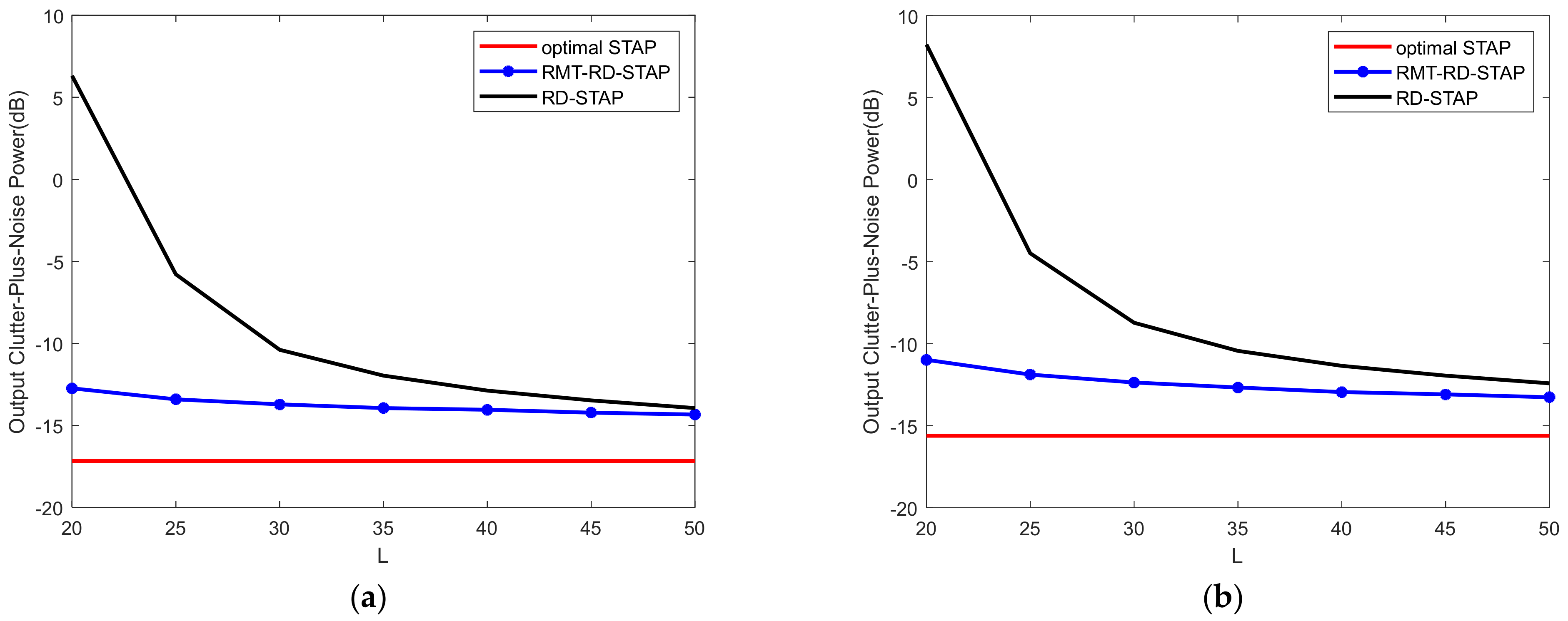
Firstly, we make a comparison of the output clutter-plus-noise powers generated by different STAP weight vectors (7), (17), and (36) for two platform velocities, V = 150 m/s and V = 300 m/s, corresponding to two local clutter DoFs, Q R d = 10 and Q R d = 12 , respectively. Figure 2 shows the output clutter-plus-noise power versus the number of training samples with f 0 t = 0.3 . It is obvious that for large L , both RD-STAP and RMT-RD-STAP have close output power. However, when the number L  of training samples becomes small, the output clutter-plus-noise power by the RD-STAP rapidly increases, whereas the power by the RMT-RD-STAP is almost kept intact. These results illustrate that the assumption of complex white Gaussian noise in reduced dimension is reasonable from the viewpoint of reducing the output clutter-plus-noise power. Comparing Figure 2a with Figure 2b, we find that the local clutter DoFs have negative effects on the output clutter-plus-noise powers. The larger the local clutter DoFs are, the larger the optimal output powers are. But the gap between the output powers produced by RMT-RD-STAP and the optimal STAP changes slightly for these two local clutter DoFs.
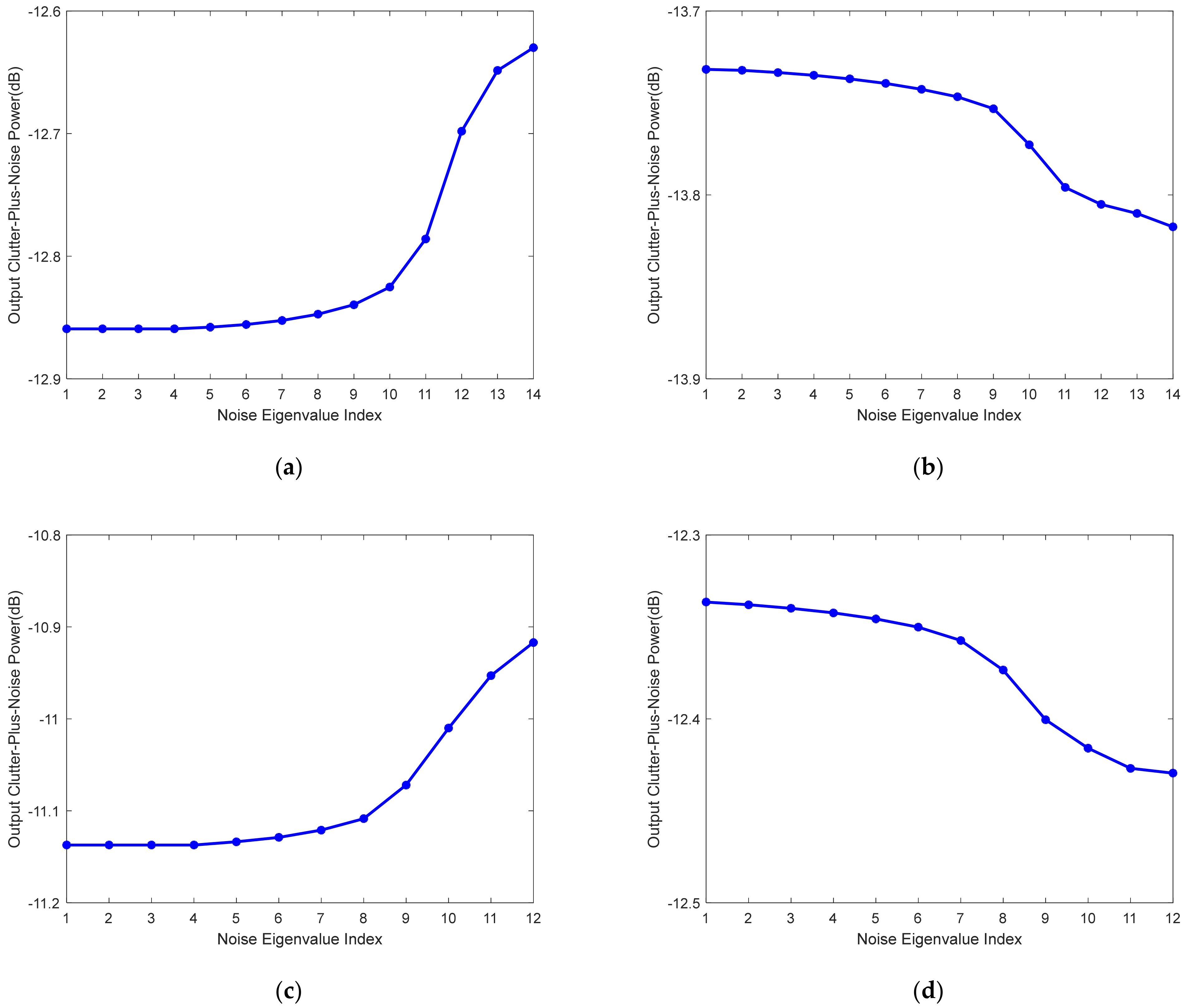
Next, we make a comparison of the output clutter-plus-noise powers under different platform velocities for RMT-RD-STAP, V = 150 m/s and V = 300 m/s, respectively. Figure 3 shows the output clutter-plus-noise power versus the noise eigenvalues with f 0 t = 0.3 , where L = 20 and L = 30 which correspond to two situations, c N r d = 3 N / 20 > 1 and c N r d = 3 N / 30 < 1 . The noise-related eigenvalues are sorted in ascending order in the figures. It is seen that when c N r d > 1 , the output clutter-plus-noise power decreases as the noise power σ decreases, and when c N r d < 1 , the output clutter-plus-noise power decreases as the noise power σ  increases. These results verify the correctness of Proposition 1. By comparing the four figures, it is obvious that the above conclusion can still be maintained when the local clutter DoFs vary.

4.2. Performance Comparisons

In this subsection, output SINR loss, the ratio of the output SINR to the SNR achieved by a matched filter in a clutter-free environment [2], is taken as a performance metric to measure different STAP algorithms. For RD-STAP, the SINR loss is given as
S I N R L o s s R D S T A P = σ n 2 N K w L r d o p t H a r d f 0 t , f 0 s 2 w L r d o p t H R w L r d o p t ,
Similar loss functions are given by optimal STAP and RMT-RD-STAP. In the following experiments, the output SINR losses are presented by averaging 1000 independent runs.
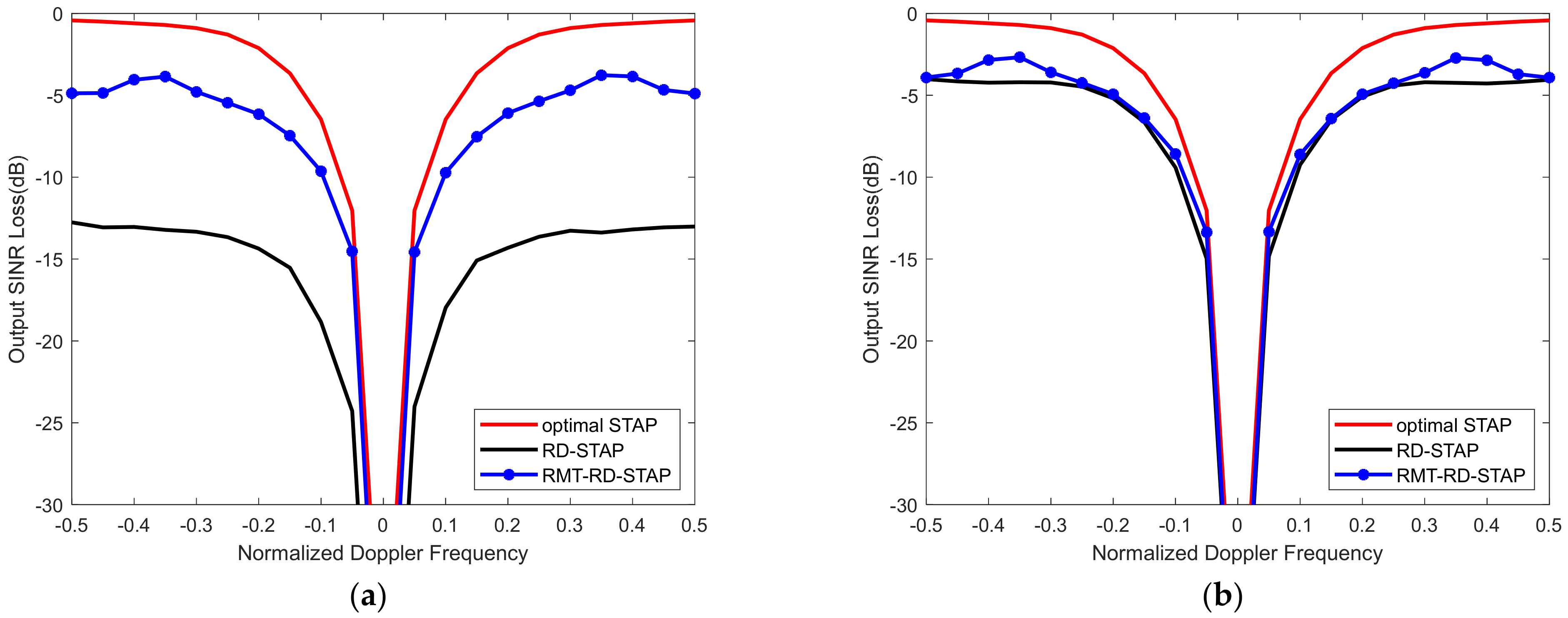
Firstly, we present the variations of the output SINR losses as the normalized Doppler frequencies for different numbers of training samples. The results are shown in Figure 4 with L = M and L = 2 M . In such cases, we choose the maximum noise-related eigenvalue of RD SCM as the noise power. The airborne platform is assumed to move at the velocity V = 150 m/s. It is seen that the RMT-RD-STAP algorithm is superior to the RD-STAP algorithm for small training samples. In Figure 4a, L = M , it is seen that RMT-RD-STAP is much superior to RD-STAP, and The SINR loss by RMT-RD-STAP decreases about 8 dB in comparison with RD-STAP. In Figure 4b, L = 2 M , which means that the number of the training samples is sufficient, and the SINR losses of both two RD-STAP algorithms decrease in comparison with that in Figure 4a. Although RMT-RD-STAP and RD-STAP have almost similar performance, RMT-RD-STAP is still slightly superior to RD-STAP.
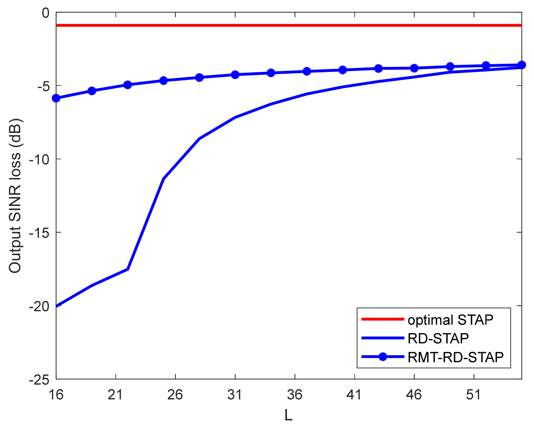
Figure 5 shows the output SINR losses versus the number of training samples L with f 0 t = 0.3 . It is seen that for large L , RMT-RD-STAP and RD-STAP achieve performance close to each other. However, as the number of training samples decreases, RMT-RD-STAP has distinct performance advantages over RD-STAP. Along with Figure 4, Figure 5 further demonstrates the advantages of the proposed RMT-RD-STAP algorithm.
Next, we present the variations of the output SINR losses as the function of normalized Doppler frequencies for different numbers of training samples. The results are shown in Figure 6 with L = M and L = 2 M , where the maximum noise-related sample eigenvalue is selected as the noise power. In the experiments, the platform is assumed to move at the velocity V = 300 m/s. Comparing Figure 6a,b, it is seen that RMT-RD-STAP is superior to RD-STAP for small-size training samples. From ref. [48], we know that the local clutter DoFs increase as the velocity increases. In comparison with Figure 4, we find that the performance of all the algorithms decreases. However, RMT-RD-STAP is still superior to RD-STAP for small-size training samples. The SINR losses of RMT-RD-STAP in L = M and L = 2 M  decrease by about 8 dB and 1 dB in comparison with RD-STAP, respectively.
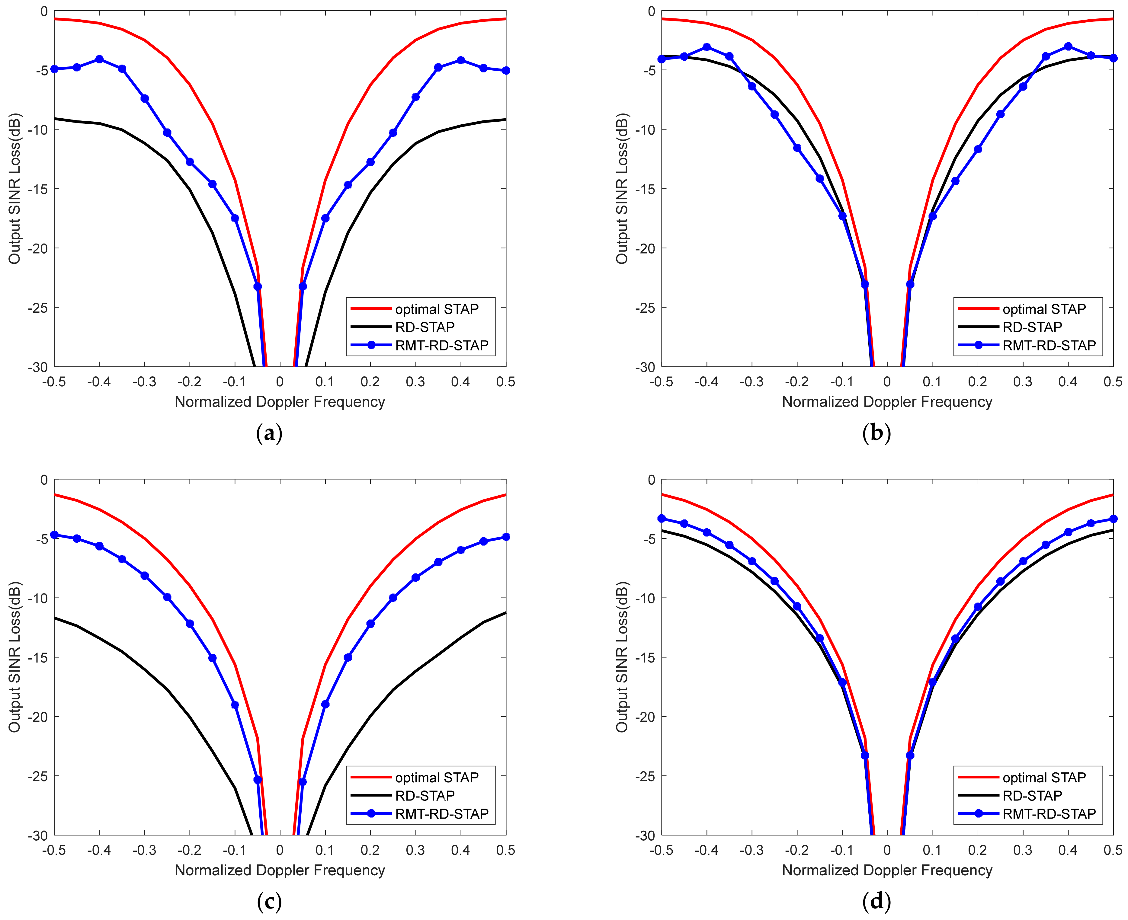
In the implementation of the proposed RMT-RD-STAP algorithm, the local clutter DoFs need to be calculated according to radar parameters and platform parameters [48]. In a real environment, these parameters often deviate from the designed ones and then the calculated local clutter DoFs are different from the real local clutter DoFs. To demonstrate the robustness of the proposed algorithm, we use Figure 7 to show the output SINR losses versus the clutter of DoF errors with f 0 t = 0.3 . In the experiments, the platform velocities are assumed to be V = 150 m/s and V = 300 m/s, and the calculated local clutter of DoFs are 10 and 12, respectively. The clutter DoF errors vary from −3 to 3. The numbers of training samples are set to be L = M and L = 2 M , respectively. It is well-known that the conventional RD-STAP is independent of the local clutter DoFs estimation, whereas the proposed RMT-RD-STAP is related to the local clutter of DoFs estimation. As observed from Figure 7, under the predesigned clutter DoF errors scope, the performance of RD-STAP is stable for all four cases. Surprisingly, we also find that the proposed RMT-RD-STAP is not sensitive to the local clutter DoFs errors and it always provides stable output SINR losses. Furthermore, the proposed RMT-RD-STAP has superior performance to RD-STAP. Specifically, the SINR losses of RMT-RD-STAP in L = M and L = 2 M , respectively, decrease by about 8 dB and 1 dB in comparison with RD-STAP.
Under real clutter circumstance, the internal clutter motion (ICM) unavoidably exists due to wind and other factors [52], which is reflected by that the increase in clutter bandwidth in temporal domain. ICM will result in the RD-STAP performance deterioration. To illustrate the robustness of the proposed RMT-RD-STAP, we consider 2% ICM, which is a general situation. Figure 8 presents the output SINR losses versus normalized Doppler frequencies with 2% ICM. In the experiments, the platform velocities are assumed to be V = 150 m/s and V = 150 m/s, and the numbers of training samples are set to be L = M and L = 2 M , respectively. We find that, under small training samples size L = M , the proposed RMT-RD-STAP still has great performance advantage in comparison with RD-STAP. On the other hand, for large training samples size L = 2 M , we find that RMT-RD-STAP and RD-STAP have almost the same performance, where RD-STAP achieves almost the optimal performance in this case according to the RMB rule.
To demonstrate the effectiveness of the proposed RMT-RD-STAP, we finally apply it to the available real clutter data, Mountain Top data, i.e., t38pre01v1CPI6 [53]. In this clutter data, the number K of transmitted pulses and the number N of array elements are 16 and 14, respectively. The PRF is 625 Hz and the distance resolution is 150 m. In the radar work time, there exist 403 range cells. We artificially add a target located in the 150-th range cell with a normalized Doppler frequency of 0.25 and the normalized spatial frequency 0.43 into the clutter data. In this case, the RD system DoFs is 42, and the local clutter DoFs is 16 in terms of [48]. Figure 9 presents the STAP output power verse the range cells with L = 45 and L = 95 . In these two cases, four range cells adjacent to the CUT are regarded as the guard cells, and 45 and 95 range cells symmetrically located around the CUT are selected as training samples, respectively. It is seen that when L = 95 , which satisfies the RMB rule, the proposed RMT-RD-STAP and RD-STAP have similar performance. However, when L = 45 , which cannot satisfy the RMB rule, the RD-STAP will show a severe false alarm in the 144-th range cell, whereas the proposed RMT-RD-STAP has a distinct performance advantage and can accurately detect the target.

5. Conclusions

In this paper, we have proposed the RMT-based RD-STAP algorithm to enhance performance in the case of finite training samples. In terms of the spiked covariance model, the proposed algorithm estimates the inverse RD CNCM by optimally manipulating its sample eigenvalues while maintaining its sample eigenvectors. By minimizing the output clutter-plus-noise power of RD-STAP, the clutter-related eigenvalues are estimated according to the clutter-related sample eigenvalues via RMT, and the noise-related eigenvalue is optimally selected from the noise-related sample eigenvalues. Benefitted from RMT, the proposed RMT-RD-STAP greatly outperforms the conventional RD-STAP when the RMB rule is not satisfied and has superior performance when the number of training samples satisfies the RMB rule.

Author Contributions

Conceptualization, D.S., S.C. and Z.L.; Funding acquisition, Z.L.; Methodology, D.S., S.C. and Z.L.; Software, D.S. and Q.F.; Supervision, S.C. and Z.L.; Validation, D.S. and Q.F.; Visualization, D.S. and Q.F.; Writing—original draft, D.S.; Writing—review and editing, S.C., F.X., and Z.L. All authors have read and agreed to the published version of the manuscript.

Funding

This research was supported in part by the National Natural Science Foundation of China under Grant 6217011933 and in part by Natural Science Foundation of Jiangsu Province under Grant BK20221486.

Conflicts of Interest

The authors declare no conflict of interest.

Appendix A

To solve the problem (37), we need to analyze the relationship between P r d w ^ r d o p t g ^ and σ . We consider the partial derivative
P r d σ = P r d g ^ i g ^ i β ^ i β ^ i α i α i σ ,
In the following, we will analyze the right four terms, respectively.
Firstly, σ α i is the sample eigenvalue of RD SCM, and α i will increase as σ decreases,
α i σ < 0 .
Secondly, in terms of the relationship β ^ i = α i 1 c N r d + α i 1 c N r d 2 4 c N r d / 2 , it is obvious that β ^ i will increase as α i increases, then
β ^ i α i > 0 .
Thirdly, from (32), we can make a replacement
ε = q = 1 Q r d c N r d k ^ r d q β ^ q a r d H f 0 t , f 0 s a r d f 0 t , f 0 s q = 1 Q r d k ^ r d q + q = 1 Q r d c N r d k ^ r d q β ^ q 2 ,
Then
g ^ i β ^ i = β ^ i 2 + 2 c N r d β ^ i + c N r d β ^ i 2 + β ^ i 2 ε β ^ i + β ^ i + c N r d β ^ i 2 + β ^ i ε β ^ i 1 ,
Practically, the clutter power in airborne radar system is generally greatly large, and the target is commonly not independent with clutter. Therefore, β ^ q is generally large, and k ^ r d q 0 . Meanwhile, it is obvious that
a r d H f 0 t , f 0 s a r d f 0 t , f 0 s q = 1 Q r d c N r d k ^ r d q β ^ q 2 q = 1 Q r d k ^ r d q ,
Then
ε 0 ,
Let us make a replacement for ε
U 1 = q = 1 q i Q r d c N r d k ^ r d q β ^ q U 2 = q = 1 q i Q r d c N r d k ^ r d q β ^ q 2 + q = 1 Q r d k ^ r d q
Then ε can be expressed as
ε = c N r d k ^ r d i β ^ i + U 1 a r d H f 0 t , f 0 s a r d f 0 t , f 0 s c N r d k ^ r d i β ^ i 2 + U 2 ,
Note that a R d H f 0 t , f 0 s a r d f 0 t , f 0 s U 2 ; therefore we have
ε c N r d k ^ r d i β ^ i + U 1 a r d H f 0 t , f 0 s a r d f 0 t , f 0 s c N r d k ^ r d i β ^ i 2 ,
Then, we can obtain the partial derivative of (A10) as
ε β ^ i = k ^ r d i c N r d β ^ i + U 1 c N r d 2 + k ^ r d i U 1 2 c N r d + k ^ r d i 2 β ^ i 2 c N r d + k ^ r d i 2 k ^ r d i c N r d β ^ i 2 β ^ i 4 c N r d 2 = k ^ r d i c N r d β ^ i 2 0 ,
Substituting (A7) and (A11) into (A5), we have
g ^ i β ^ i β ^ i 2 + 2 c N r d β ^ i + c N r d β ^ i β ^ i + 1 2 β ^ i + c N r d β ^ i 2 + β ^ i = c N r d 1 β ^ i + 1 2 ,
According to (A12), notice that the relationship between g ^ i and β ^ i depends upon c N r d . If c N r d > 1 , i.e., L < M , g ^ i / β ^ i > 0 , otherwise g ^ i / β ^ i < 0 .
Finally, we consider that P r d / g ^ i . P r d can be approximated as
P r d = σ a r d H f 0 t , f 0 s I M + q = 1 Q r d g ^ q d q d q H R r d I M + i = 1 Q r d g ^ i d i d i H a r d f 0 t , f 0 s a r d H f 0 t , f 0 s I M + i = 1 Q r d g ^ i d i d i H a r d f 0 t , f 0 s 2 σ a r d H f 0 t , f 0 s a r d f 0 t , f 0 s + i = 1 Q r d k ^ r d i β i + i = 1 Q r d s r d i 2 k ^ r d i β i g ^ i * + 1 s r d i 2 a r d H f 0 t , f 0 s a r d f 0 t , f 0 s + i = 1 Q r d s r d i k ^ r d i g ^ i * + 1 s r d i 2 = σ P 1 + s r d i 2 k ^ r d i β i g ^ i * + 1 s r d i 2 P 2 + s r d i k ^ r d i g ^ i * + 1 s r d i 2
where
P 1 = a r d H f 0 t , f 0 s a r d f 0 t , f 0 s + i = 1 Q r d k ^ r d i β i + q = 1 q i Q r d s r d q 2 k ^ r d q β q g ^ q + 1 s r d q 2 P 2 = a r d H f 0 t , f 0 s a r d f 0 t , f 0 s + q = 1 q i Q r d s r d q k ^ r d q g ^ q + 1 s r d q
Then, we can obtain the partial derivative of (A13) as
P g ^ i σ 2 s r d i 2 k ^ r d i β i g ^ i + 1 s r d i P 2 + s r d i k ^ r d i g ^ i + 1 s r d i 2 s r d i k ^ r d i P 1 + s r d i 2 k ^ r d i β i g ^ i + 1 s r d i 2 P 2 + s r d i k ^ r d i g ^ i + 1 s r d i 3 ,
As the clutter power is commonly high, we have s r d i = 1 c N r d / β i 2 / 1 + c N r d / β i 1 . Substituting (32) into (A15), we have
P g ^ i σ 2 k ^ r d i β i g ^ i + 1 P 2 + k ^ r d i g ^ i + 1 2 k ^ r d i P 1 + k ^ r d i β i g ^ i + 1 2 P 2 + k ^ r d i g ^ i + 1 3 = σ 2 k ^ r d i β i g ^ i + 1 P 2 P 1 P 2 + k ^ r d i g ^ i + 1 3
The denominator of (A16) is larger than 0 evidently, then the sign of (A16) completely depends on the numerator of (A16). Note that
2 k ^ r d i β i g ^ i + 1 P 2 P 1 a r d H f 0 t , f 0 s a r d f 0 t , f 0 s c N r d i = 1 Q r d k ^ r d i β i .
Therefore, it is obvious that P r d / g ^ i < 0 .
In summary, if c N r d > 1 , P r d / σ > 0 , the output clutter-plus-noise power decreases as σ decreases; if c N r d < 1 , P r d / σ < 0 , the output clutter-plus-noise power decreases as σ increases.

References

  1. Brennan, L.E.; Reed, L.S. Theory of adaptive radar. IEEE Trans. Aerosp. Electron. Syst. 1973, AES-9, 237–252. [Google Scholar] [CrossRef]
  2. Ward, J. Space-Time Adaptive Processing for Airborne Radar; Technical Report 1015; MIT Lincoln Lab.: Lexington, MA, USA, 1994. [Google Scholar]
  3. Melvin, W.L. A STAP overview. IEEE Aerosp. Electron. Syst. Mag. 2004, 19, 19–35. [Google Scholar] [CrossRef]
  4. Reed, I.S.; Mallett, J.D.; Brennan, L.E. Rapid convergence rate in adaptive arrays. IEEE Trans. Aerosp. Electron. Syst. 1974, AES-10, 853–863. [Google Scholar] [CrossRef]
  5. Klemm, R. Principles of Space-Time Adaptive Processing, 3rd ed.; IET: London, UK, 2006. [Google Scholar]
  6. Guerci, J.R. Space-Time Adaptive Processing for Radar; Artech House: Norwood, MA, USA, 2003. [Google Scholar]
  7. Yang, Z.; Li, X.; Wang, H.; Jiang, W. On Clutter Sparsity Analysis in Space–Time Adaptive Processing Airborne Radar. IEEE Geosci. Remote Sens. Lett. 2013, 10, 1214–1218. [Google Scholar] [CrossRef]
  8. Sen, S. Low-Rank Matrix Decomposition and Spatio-Temporal Sparse Recovery for STAP Radar. IEEE J. Sel. Top. Signal Process. 2015, 9, 1510–1523. [Google Scholar] [CrossRef]
  9. Yang, Z.; de Lamare, R.C.; Li, X. L1-Regularized STAP algorithms with a generalized sidelobe canceler architecture for airborne radar. IEEE Trans. Signal Process. 2012, 60, 674–686. [Google Scholar] [CrossRef]
  10. Zhang, W.; An, R.; He, N.; He, Z.; Li, H. Reduced dimension STAP based on sparse recovery in heterogeneous clutter environments. IEEE Trans. Aerosp. Electron. Syst. 2020, 56, 785–795. [Google Scholar] [CrossRef]
  11. Guerci, J.; Baranoski, E. Knowledge-aided adaptive radar at DARPA: An overview. IEEE Signal Process. Mag. 2006, 23, 41–50. [Google Scholar] [CrossRef]
  12. Besson, O.; Tourneret, J.-Y.; Bidon, S. Knowledge-Aided Bayesian Detection in Heterogeneous Environments. IEEE Signal Process. Lett. 2007, 14, 355–358. [Google Scholar] [CrossRef]
  13. Riedl, M.; Potter, L.C. Knowledge-Aided Bayesian Space-Time Adaptive Processing. IEEE Trans. Aerosp. Electron. Syst. 2018, 54, 1850–1861. [Google Scholar] [CrossRef]
  14. Riedl, M.; Potter, L.C. Multimodel Shrinkage for Knowledge-Aided Space-Time Adaptive Processing. IEEE Trans. Aerosp. Electron. Syst. 2018, 54, 2601–2610. [Google Scholar] [CrossRef]
  15. Duan, K.; Chen, H.; Xie, W.; Wang, Y. Deep learning for high-resolution estimation of clutter angle-Doppler spectrum in STAP. IET Radar Sonar Navig. 2022, 16, 193–207. [Google Scholar] [CrossRef]
  16. Zou, B.; Wang, X.; Feng, W.; Zhu, H.; Lu, F. DU-CG-STAP Method Based on Sparse Recovery and Unsupervised Learning for Airborne Radar Clutter Suppression. Remote Sens. 2022, 14, 3472. [Google Scholar] [CrossRef]
  17. Zhu, H.; Feng, W.; Feng, C.; Zou, B.; Lu, F. Deep Unfolding Based Space-Time Adaptive Processing Method for Airborne Rada. J. Radars 2022, 11, 1–16. [Google Scholar]
  18. DiPietro, R.C. Extended factored space-time processing for airborne radar systems. In Proceedings of the Conference Record of the Twenty-Sixth Asilomar Conference on Signals, Systems & Computers, Pacific Grove, CA, USA, 26–28 October 1992; pp. 425–430. [Google Scholar]
  19. Sarkar, T.K.; Wang, H.; Park, S.; Adve, R.; Koh, J.; Kim, K.; Zhang, Y.; Wicks, M.; Brown, R. A deterministic least-squares approach to space-time adaptive processing (STAP). IEEE Trans. Antennas Propag. 2001, 49, 91–103. [Google Scholar] [CrossRef]
  20. Brown, R.; Schneible, R.; Wicks, M.; Wang, H.; Zhang, Y. STAP for clutter suppression with sum and difference beams. IEEE Trans. Aerosp. Electron. Syst. 2000, 36, 634–646. [Google Scholar] [CrossRef]
  21. Zhang, W.; He, Z.; Li, J.; Liu, H.; Sun, Y. A Method for Finding Best Channels in Beam-Space Post-Doppler Reduced-Dimension STAP. IEEE Trans. Aerosp. Electron. Syst. 2014, 50, 254–264. [Google Scholar] [CrossRef]
  22. Klemm, R. Adaptive airborne MTI: An auxiliary channel approach. IEE Proc. F Commun. Radar Signal Process. 1987, 134, 269–276. [Google Scholar] [CrossRef]
  23. Wang, H.; Cai, L. On adaptive spatial-temporal processing for airborne surveillance radar systems. IEEE Trans. Aerosp. Electron. Syst. 1994, 30, 660–670. [Google Scholar] [CrossRef]
  24. Karoui, N.E. Spectrum estimation for large dimensional covariance matrices using random matrix theory. Ann. Statist. 2008, 36, 2757–2790. [Google Scholar] [CrossRef]
  25. Daniels, R.; Kass, M.J. Shrinkage estimators for covariance matrices. Biometrics 2001, 57, 1173–1184. [Google Scholar] [CrossRef] [PubMed]
  26. Fan, J.; Fan, Y.; Lv, J. High dimensional covariance matrix estimation using a factor model. J. Econ. 2008, 147, 186–197. [Google Scholar] [CrossRef]
  27. Yang, L.; McKay, M.R.; Couillet, R. High-Dimensional MVDR Beamforming: Optimized Solutions Based on Spiked Random Matrix Models. IEEE Trans. Signal Process. 2018, 66, 1933–1947. [Google Scholar] [CrossRef]
  28. Bai, Z.; Silverstein, J.W. Spectral Analysis of Large Dimensional Random Matrices; Springer: New York, NY, USA, 2010; Volume 20. [Google Scholar]
  29. Silverstein, J.; Choi, S. Analysis of the Limiting Spectral Distribution of Large Dimensional Random Matrices. J. Multivar. Anal. 1995, 54, 295–309. [Google Scholar] [CrossRef]
  30. Schott, J.R. Asymptotics of eigenprojections of correlation matrices with some applications in principal components analysis. Biometrika 1997, 84, 327–337. [Google Scholar] [CrossRef]
  31. Bai, Z.D.; Silverstein, J.W. No eigenvalues outside the support of the limiting spectral distribution of large-dimensional sample covariance matrices. Ann. Probab. 1998, 26, 316–345. [Google Scholar] [CrossRef]
  32. Silverstein, J. Strong Convergence of the Empirical Distribution of Eigenvalues of Large Dimensional Random Matrices. J. Multivar. Anal. 1995, 55, 331–339. [Google Scholar] [CrossRef]
  33. Ledoit, O.; Wolf, M. Spectrum estimation: A unified framework for covariance matrix estimation and PCA in large dimensions. J. Multivar. Anal. 2015, 139, 360–384. [Google Scholar] [CrossRef]
  34. Ledoit, O.; Wolf, M. Nonlinear shrinkage of the covariance matrix for portfolio selection: Markowitz meets Goldilocks. Rev. Financ. Stud. 2017, 30, 4349–4388. [Google Scholar] [CrossRef]
  35. Girko, V. Asymptotic behavior of eigenvalues of empirical covariance matrices. Theory Probab. Math. Stat. 1992, 44, 37–44. [Google Scholar]
  36. Rubio, F.; Mestre, X.; Palomar, D.P. Performance Analysis and Optimal Selection of Large Minimum Variance Portfolios Under Estimation Risk. IEEE J. Sel. Top. Signal Process. 2012, 6, 337–350. [Google Scholar] [CrossRef]
  37. Anderson, T.W. Asymptotic Theory for Principal Component Analysis. Ann. Math. Stat. 1963, 34, 122–148. [Google Scholar] [CrossRef]
  38. Gupta, R. Asymptotic theory for principal component analysis in the complex case. J. Indian Statist. Assoc. 1965, 3, 97–106. [Google Scholar]
  39. Marcenko, V.A.; Pastur, L.A. Distribution of Eigenvalues for Some Sets of Random Matrices. Math. USSR-Sb. 1967, 1, 457–483. [Google Scholar] [CrossRef]
  40. Baik, J.; Arous, G.B.; Péché, S. Phase transition of the largest eigenvalue for nonnull complex sample covariance matrices. Ann. Probab. 2005, 33, 1643–1697. [Google Scholar] [CrossRef]
  41. Baik, J.; Silverstein, J.W. Eigenvalues of large sample covariance matrices of spiked population models. J. Multivar. Anal. 2006, 97, 1382–1408. [Google Scholar] [CrossRef]
  42. Paul, D. Asymptotics of sample eigenstructure for a large dimensional spiked covariance model. Statist. Sin. 2007, 17, 1617–1642. [Google Scholar]
  43. Couillet, R. Robust spiked random matrices and a robust G-MUSIC estimator. J. Multivar. Anal. 2015, 140, 139–161. [Google Scholar] [CrossRef]
  44. Robinson, B.D.; Malinas, R.; Hero, A.O. Space-Time Adaptive Detection at Low Sample Support. IEEE Trans. Signal Process. 2021, 69, 2939–2954. [Google Scholar] [CrossRef]
  45. Combernoux, A.; Pascal, F.; Lesturgie, M.; Ginolhac, G. Performances of low rank detectors based on random matrix theory with application to STAP. In Proceedings of the 2014 International Radar Conference, Lille, France, 13–17 October 2014; pp. 1–4. [Google Scholar]
  46. Pafka, S.; Kondor, I. Noisy covariance matrices and portfolio optimization II. Phys. A Stat. Mech. Its Appl. 2003, 319, 487–494. [Google Scholar] [CrossRef]
  47. Pafka, S.; Kondor, I. Estimated correlation matrices and portfolio optimization. Phys. A Stat. Mech. Table Its Appl. 2004, 343, 623–634. [Google Scholar] [CrossRef]
  48. Zhang, Z.; Xie, W.; Hu, W.; Yu, W. Local degrees of freedom of airborne array radar clutter for STAP. IEEE Geosci. Remote Sens. Lett. 2009, 6, 97–101. [Google Scholar]
  49. Mestre, X. On the Asymptotic Behavior of the Sample Estimates of Eigenvalues and Eigenvectors of Covariance Matrices. IEEE Trans. Signal Process. 2008, 56, 5353–5368. [Google Scholar] [CrossRef]
  50. Mestre, X. Improved Estimation of Eigenvalues and Eigenvectors of Covariance Matrices Using Their Sample Estimates. IEEE Trans. Inf. Theory 2008, 54, 5113–5129. [Google Scholar] [CrossRef]
  51. Couillet, R.; Debbah, M. Random Matrix Methods for Wireless Communications; Cambridge Univ. Press: Cambridge, UK, 2011. [Google Scholar]
  52. Melvin, W.L.; Showman, G.A. An approach to knowledge-aided covariance estimation. IEEE Trans. Aerosp. Electron. Syst. 2006, 42, 1021–1042. [Google Scholar] [CrossRef]
  53. Titi, G.; Marshall, D. The ARPA/NAVY Mountaintop Program: Adaptive signal processing for airborne early warning radar. In Proceedings of the IEEE International Conference on Acoustics, Speech, and Signal Processing Conference Proceedings, Atlanta, GA, USA, 9 May 1996; IEEE: Piscataway Township, NJ, USA, 2002; Volume 2, pp. 1165–1168. [Google Scholar]
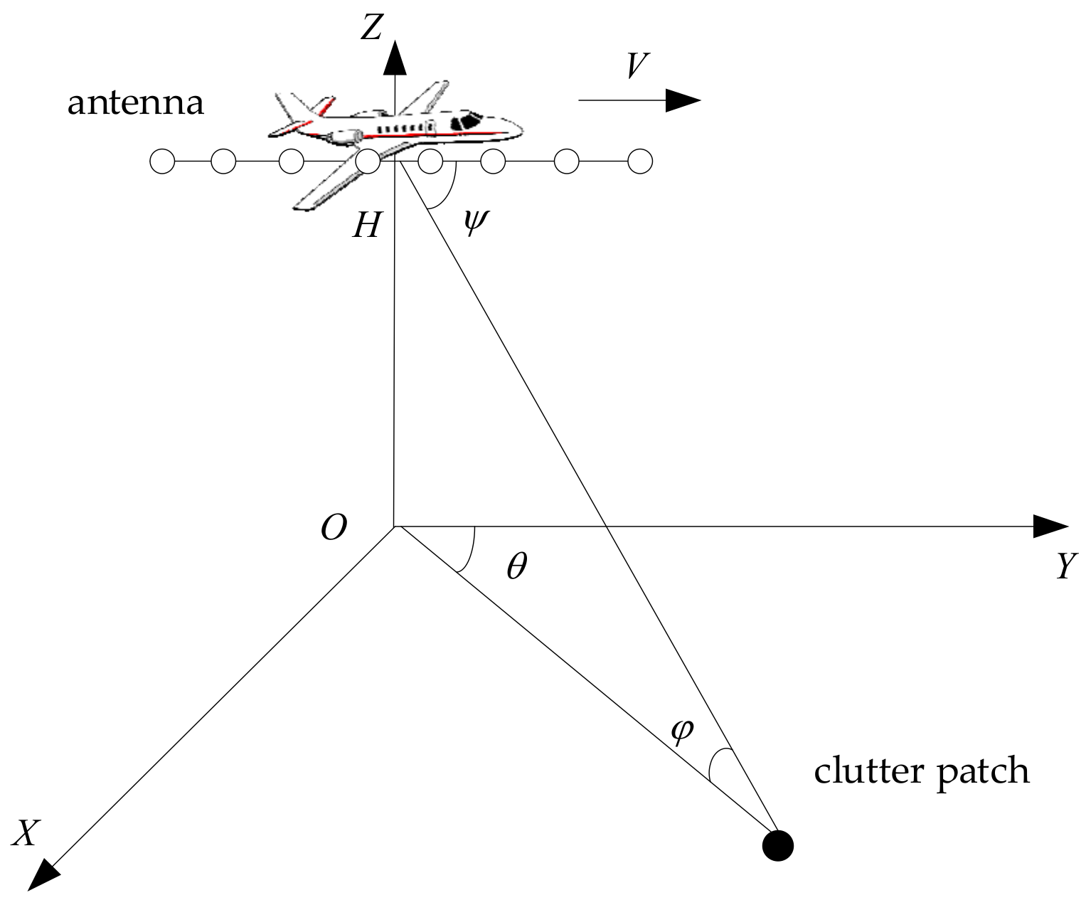
Figure 1. Side-looking airborne radar geometry relationship.
Remotesensing 14 03959 g001
Figure 2. The output clutter-plus-noise power against the number L of the training samples. (a) V = 150 m/s and (b) V = 300 m/s.
Remotesensing 14 03959 g002
Figure 3. The output clutter-plus-noise powers versus the noise eigenvalues. (a) V = 150 m/s, L = 20 ; (b) V = 150 m/s, L = 30 ; (c) V = 300 m/s, L = 20 ; (d) V = 300 m/s, L = 30 .
Remotesensing 14 03959 g003
Figure 4. Output SINR losses versus normalized Doppler frequencies with V = 150 m/s. (a) L = M training samples and (b) L = 2 M training samples.
Remotesensing 14 03959 g004
Figure 5. Output SINR losses versus the number L of the training samples.
Remotesensing 14 03959 g005
Figure 6. Output SINR losses versus normalized Doppler frequencies with V = 300 m/s. (a) L = M training samples and (b) L = 2 M training samples.
Remotesensing 14 03959 g006
Figure 7. Output SINR losses versus clutter DoF errors. (a) V = 150 m/s, L = M ; (b) V = 150 m/s, L = 2 M ; (c) V = 300 m/s, L = M and (d) V = 300 m/s, L = 2 M .
Remotesensing 14 03959 g007
Figure 8. Output SINR losses versus normalized Doppler frequencies with 2% ICM. (a) V = 150 m/s, L = M ; (b) V = 150 m/s, L = 2 M ; (c) V = 300 m/s, L = M and (d) V = 300 m/s, L = 2 M .
Remotesensing 14 03959 g008
Figure 9. Output power versus range cell. (a) L = 45 training samples and (b) L = 95 training samples.
Remotesensing 14 03959 g009
Table 1. Parameters used in the experiment scenarios.
ParameterValueUnit
Height6000m
Wavelength0.3m
Array number8/
Pulse number8/
PRF2000Hz
CNR30dB
Publisher’s Note: MDPI stays neutral with regard to jurisdictional claims in published maps and institutional affiliations.