Article

On the Efficient Implementation of Sparse Bayesian Learning-Based STAP Algorithms

1
National Lab of Radar Signal Processing, Xidian University, Xi’an 710071, China
2
School of Electronics and Communication Engineering, Sun Yat-sen University, Guangzhou 510275, China
*
Author to whom correspondence should be addressed.
Remote Sens. 2022, 14(16), 3931; https://doi.org/10.3390/rs14163931
Submission received: 13 July 2022 / Revised: 9 August 2022 / Accepted: 11 August 2022 / Published: 13 August 2022
(This article belongs to the Special Issue Small or Moving Target Detection with Advanced Radar System)

Abstract

:
Sparse Bayesian learning-based space–time adaptive processing (SBL-STAP) algorithms can achieve superior clutter suppression performance with limited training sample support in practical heterogeneous and non-stationary clutter environments. However, when the system has high degrees of freedom (DOFs), SBL-STAP algorithms suffer from high computational complexity, since the large-scale matrix calculations and the inversion operations of large-scale covariance matrices are involved in the iterative process. In this article, we consider a computationally efficient implementation for SBL-STAP algorithms. The efficient implementation is based on the fact that the covariance matrices that need to be updated in the iterative process of the SBL-STAP algorithms have a Hermitian Toplitz-block-Toeplitz (HTBT) structure, with the result being that the inverse covariance matrix can be expressed in closed form by using a special case of the Gohberg–Semencul (G-S) formula. Based on the G-S-type factorization of the inverse covariance matrix and the structure of the used dictionary matrix, we can perform almost all operations in the SBL-STAP algorithms by 2-D FFT/IFFT. As a result, compared with the original SBL-STAP algorithms, even for moderate data sizes, the proposed algorithms can directly reduce the computational load by about two orders of magnitudes without any performance loss. Finally, simulation results validate the effectiveness of the proposed algorithms.

Graphical Abstract

1. Introduction

Space–time adaptive processing (STAP) [1,2,3,4] adopts two-dimensional joint adaptive filtering in the space and time domains to achieve effective filtering of clutter, and it is a key technology for radar clutter suppression and target detection using various types of motion platforms. The self-adaptation of STAP technology is reflected in the accurate perception of the external clutter environment, which relies on the real-time acquisition of the clutter plus noise covariance matrix (CNCM) of the cell under test (CUT). However, the CNCM is usually unknown in practical applications and need to be estimated on the basis of the independent and identically distributed (IID) training samples. To achieve an output signal-to-clutter-plus-noise ratio (SCNR) loss within 3 dB, according to the well-known Reed–Mallett–Brennan (RMB) rule [5], the number of IID training samples required to estimate CNCM should be greater than twice the system’s degrees of freedom (DOFs). In fact, airborne radars usually work in heterogeneous and non-stationary clutter environments, and it is difficult to obtain enough IID training samples.
Sparse recovery (SR) techniques [6,7,8,9,10,11,12,13,14,15,16,17,18,19,20,21,22,23] can use limited training samples to reconstruct signals with high precision, and this feature is exactly in line with the requirement of using as few observation samples as possible to accurately describe the clutter characteristics in the STAP. Thus, SR-based STAP (SR-STAP) techniques [24,25,26,27,28,29] have inherent advantages for CNCM estimation in fast-changing clutter environments. In recent years, many SR techniques have been applied to airborne radar clutter suppression processing to improve the detection performance of slow moving targets under the condition that there are not enough training samples in practice. The greedy algorithms [10,11,12,13] iteratively select atoms from the dictionary and calculate the corresponding sparse coefficients, so that the difference between the linear combination of these atoms and the observed data is gradually reduced. The convex optimization (CVX) algorithms [14,15,16,17,18,19] relax the 0 - norm optimization problem into a CVX problem, and use the properties of the CVX function to obtain the sparse coefficient vector. The focal underdetermined system solver (FOCUSS) algorithms [20,21] use iterative p - norm ( 0 < p < 1 ) optimization to approximate 0 - norm optimization and transform the 0 - norm optimization problem into a weighted minimum norm least square problem. The iterative adaptive approach (IAA) [22,23] is a non-parametric algorithm based on iterative weighted least squares approach. Although these SR techniques have great advantages in combination with STAP, they suffer from some drawbacks: the greedy algorithms may fail when there has a strong correlation between the atoms of the dictionary, resulting in poor sparse coefficient solutions. The performance of CVX algorithms and FOCUSS algorithms is closely related to the choice of regularization parameters and the IAA algorithms easily suffer from severe performance degradation in the non-ideal case.
Sparse Bayesian learning (SBL) [30,31,32,33,34,35], proposed by Tipping, is a popular SR technique for signal reconstruction. Compared with other SR algorithms, SBL does not require setting regularization parameters and can be used to obtain a sparser global optimal solution. Moreover, SBL can still achieve favorable performance when the dictionary possesses a high coherence. Due to their superior performance, SBL-based STAP (SBL-STAP) algorithms with multiple measurement vectors (MMV) [36,37,38,39,40,41,42,43] have been widely researched. However, in MMV-based SBL-STAP (MSBL-STAP) algorithms, an iterative procedure that converges very slowly is utilized to reconstruct the CNCM. Additionally, inversion operations of the large-scale covariance matrices and several large-scale matrix calculations are involved in each iteration, which is quite computationally expensive for MSBL-STAP algorithms in practical applications. To tackle this problem, many efficient MSBL-STAP methods have been developed. In [44], a fast tensor-based three-dimensional MSBL-STAP (TMSBL-STAP) algorithm was proposed, in which the large-scale matrix calculation was decomposed into small-scale matrix calculation by utilizing the Kronecker structure of the data. However, this algorithm only relieves a small part of the computational burden. In [45], by combining a simple approximation term, a fast-converging MSBL-STAP (MFCSBL-STAP) algorithm was proposed to improve the convergence of MSBL-STAP algorithm. In [46], an MSBL-STAP algorithm based on the iterative reweighed 2 , 1 - norm ( IR 2 , 1 - MSBL - STAP ) was proposed, and the experiments showed that the algorithm had great convergence performance. Compared with the basic MSBL-STAP algorithms, these two algorithms can greatly improve the convergence speed and exhibit a comparable or even a better reconstruction accuracy. However, they ignore the core problem that there exist large-scale covariance matrix inversion operations and large-scale matrix calculations in each iteration of these MSBL-STAP algorithms, which have high computational complexity.
In this article, we propose several efficient MSBL-STAP algorithms based on the G-S factorization [47] for airborne radar in the case of uniformly spaced linear array (ULA) and a constant pulse repetition frequency (PRF). In our proposed algorithms, based on the fact that the inverse of the Hermitian Toplitz-block-Toeplitz (HTBT) matrix has low displacement ranks [48] and can be written in a G-S factorization-based form, an equivalent G-S factorization-based method is utilized to efficiently calculate the inverse covariance matrices in the iterative process of the MSBL-STAP algorithms. Then, by utilizing the property whereby the dictionary matrix is the Kronecker product of two Fourier matrices and the obtained G-S-type factors of the inverse covariance matrix, many large-scale matrices in the iterative process of the MSBL-STAP algorithms can be efficiently computed by using 2D-FFT/IFFT [49].
The main contributions of this paper can be listed as follows:
(a) The algorithm efficiency is the focus of this paper; in this paper, several computationally effective MSBL-STAP algorithms based on G-S factorization are proposed. In our proposed algorithms, utilizing the G-S factorization of the inverse of the Hermitian Toplitz-block-Toeplitz matrix and the structure of the dictionary matrix, almost all the processing procedures of the original MSBL-STAP algorithms can be implemented with fast FFT/IFFT. Compared with the original MSBL-STAP algorithms, these proposed algorithms can directly reduce the computational complexity by several orders of magnitude without any performance loss.
(b) A detailed comparison is presented to show the computational complexity of the proposed computationally efficient MSBL-STAP algorithms and the original MSBL-STAP algorithms and other SR-STAP algorithms.
(c) A detailed comparative analysis of our proposed algorithms, including the convergence speed, the clutter suppression performance and the target detection performance, with the original MSBL-STAP algorithms and other SR-STAP algorithms is carried out.
The rest of the paper is organized as follows. In Section 2, the general space–time sparse signal model is introduced. In Section 3, a brief review of the traditional MSBL-STAP algorithms is provided. In Section 4, we give a detail introduction of the proposed algorithms. In Section 5, simulation results are provided to demonstrate the computational efficiency, the clutter suppression performance and the target detection performance of the proposed algorithms. Final conclusions are given in Section 6.
Notation: Boldface lowercase letters denote vectors and boldface uppercase letters denote matrices. + represents the nonnegative real field and represents the complex field. ( ) , ( ) T and ( ) H represent the complex conjugate, transpose and conjugate transpose, respectively. The symbol denotes the Kronecker product. 0 represents a zero vector/matrix. I N K denotes the N K × N K identity matrix. d i a g ( ) represents a diagonal matrix with entries of a vector on the diagonal or a vector is made up of all the elements on the diagonal of a matrix. The symbol denotes a definition. F denotes the Frobenius norm. The symbol ~ above a matrix represents reversing the elements in a matrix first by row, then by column. F 2 D ( ) N , K and I F 2 D ( ) N , K denote the N - and K - point 2-D FFT and IFFT operations.

2. Signal Model

Consider an airborne pulsed-Doppler radar system employing a side-looking ULA consisting of N elements. The interelement spacing is d = λ / 2 , where λ is the wavelength. K pulses are transmitted at a constant PRF during a coherent processing interval (CPI). Then, the space–time sparse signal model in the MMV case can be written as
Y = D X + N
where Y = [ y 1 , y 2 , , y L ] N K × L is the received clutter plus noise data, X = [ x 1 , x 2 , , x L ] N s K d × L is the unknown angle-Doppler profile to be recovered with each row representing a possible clutter component, N = [ n 1 , n 2 , , n L ] N K × L is the zero mean noise matrix with covariance matrix σ 2 I , σ 2 is the noise power and I is the identity matrix, D = S t S s = [ v 1 , v 2 , , v N s K d ] N K × N s K d is the space–time dictionary matrix, v m ( m = 1 , 2 , , N s K d ) is the spatial-temporal steering vector of the m th grid point of the whole angle-Doppler plane, N s = ρ s N ( ρ s > 1 ) is the number of normalized spatial frequency bins and K d = ρ d K ( ρ d > 1 ) is the number of normalized Doppler frequency bins, S s = [ s s , 1 , s s , 2 , , s s , N s ] N × N s and S t = [ s t , 1 , s t , 2 , , s t , K d ] K × K d are two Fourier matrices, s s , n and s t , k are the spatial and temporal steering vectors, given by
s s , n = { 1 , exp [ j 2 π f s , n ] , , exp [ j 2 π ( N 1 ) f s , n ] } T ,   n = 1 , 2 , , N s
s t , k = { 1 , exp [ j 2 π f d , k ] , , exp [ j 2 π ( K 1 ) f d , k ] } T ,   k = 1 , 2 , , K d
where   f s , n = ( n 1 ) / N s is the normalized spatial frequency of the n th angle grid point and f d , k = ( k 1 ) / K d is the normalized Doppler frequency of the k th Doppler grid point.

3. A Brief Review of the Traditional MSBL-STAP Algorithms

In this section, firstly, we give a brief review of the basic MSBL-STAP algorithm proposed by Duan [36]; then, we directly give the pseudocodes of two fast-converging MSBL-STAP algorithms for the brevity of the article. According to the signal model in (1), the Gaussian likelihood function of the measurement can be denoted as
p ( Y | X ; σ 2 ) = ( π σ 2 ) N K L exp ( σ 2 Y D X F 2 )
Suppose that each column in X obeys a complex Gaussian prior, i.e.,
x l N ( 0 , Γ ) ,   l = 1 , 2 , , L
where Γ = diag ( γ ) , γ = [ γ 1 , γ 2 , , γ N s K d ] T are the unknown variance parameters which controlling the prior covariance of x l . Then, we can obtain the prior probability density function (PDF) of X
p ( X ; Γ ) = π N s K d L | Γ | L exp ( l = 1 L x l H Γ 1 x l )
If the above prior distributions are obtained, we can obtain the posterior PDF of X by using Bayesian estimation methods [30]:
p ( X | Y ; Γ , σ 2 ) = π N s K d L | Σ | L exp [ l = 1 L ( x l μ l ) H Σ 1 ( x l μ l ) ]
where μ = [ μ 1 , μ 2 , , μ L ] and Σ are the posteriori mean matrix and the posteriori covariance matrix respectively, given by
Σ = Γ Γ D H R 1 D Γ
μ = Γ D H R 1 Y
where R = σ 2 I N K + D Γ D H is the covariance matrix to be inverted in each iteration of the basic MSBL-STAP algorithm. Then, we use the expectation-maximization (EM) [30] method to estimated γ m   ( m = 1 , 2 , , N s K d ) and σ 2 , which are unknown hyperparameters in μ . We have
γ m t + 1 = 1 L l = 1 L ( μ l , m t ) 2 + Σ m , m t
( σ 2 ) t + 1 = ( 1 / L ) Y D μ t F 2 N K m = 1 N s K d ( 1 Σ m , m t / γ m t )
where the superscript t indicates the t th iteration, μ l , m t is the m th component of μ l t , Σ m , m t is the m th component of the main diagonal of Σ t . In fact, by updating and iterating μ , we can finally obtain the optimal sparse solution X ^ when a predefined convergence criterion is satisfied:
μ t μ t 1 μ t < δ
where δ is a small enough positive value. Then, the angle-Doppler profile X ^ can be given by
X ^ = μ
Then, we can estimate the CNCM by the formula
R c + n = 1 L l = 1 L m = 1 N s K d | x ^ l m | 2 v m v m H + α σ 2 I N K
where x ^ l m is the m th element of the l th column of X ^ and α is a positive loading factor. Finally, we can obtain the optimal STAP weight vector based on the linearly constrained minimum variance (LCMV) principle, given by
w opt = R c + n 1 v t v t H R c + n 1 v t
where v t is the spatial-temporal steering vector of the target.
The MFCSBL-STAP algorithm [45] proposed by Wang and the IR 2 , 1 - MSBL - STAP [46] algorithm proposed by Liu significantly accelerate the convergence speed of the basic MSBL-STAP algorithm proposed by Duan [36]. For the sake of brevity in this article, here we will not describe these two algorithms in detail. Instead, we give the pseudocodes of these two algorithms in Table 1 and Table 2.

4. Proposed Algorithms

From the procedures of the basic MSBL-STAP algorithm, the MFCSBL-STAP algorithm and the IR 2 , 1 - MSBL - STAP algorithm, it can be observed that we need to calculate the product of many large-scale matrices and the inverse of the covariance matrix R in each iteration. The size of R is N K × N K , i.e., the computational complexity in each iteration of these MSBL-STAP algorithms is at least o ( ( N K ) 3 ) . Thus, the MSBL-STAP algorithms have a computational complexity that grows rapidly with the DOFs of the STAP system, which hinders its application in many practical problems with even moderately large data sets. To tackle this question, in this section, an efficient G-S factorization-based implementation for these MSBL-STAP algorithms is proposed.
From (1), we know that the space–time dictionary matrix D is the Kronecker product of two Fourier matrices S t and S s . The k N s + n + 1   column of D can be written as
D ( ω k , ω n ) = s t ( ω k ) s s ( ω n )
where
s t ( ω k ) = { 1 , exp [ j ω k ] , , exp [ j ( K 1 ) ω k ] } T
s s ( ω n ) = { 1 , exp [ j ω n ] , , exp [ j ( N 1 ) ω n ] } T
where ω k = 2 π k / K d , k = 0 , 1 , , K d 1 , ω n = 2 π n / N s , n = 1 , 2 , , N s . The covariance matrix R in each iteration of the MSBL-STAP algorithms can be represented by
R = σ 2 I + Q
where Q = D Γ D H and can be represented by
Q = [ Q 0 Q 1 H Q K 1 H Q 1 Q 0 Q 1 H Q K 1 Q 1 Q 0 ]
From (20), we know that Q is a HTBT matrix [50,51], and each submatrix Q j 1 can be calculated by
Q j 1 = M 0 + e j 2 π 1 K d j 1 M 1 + + e j 2 π K d 1 K d j 1 M K d 1  
where j 1 = 0 , 1 , , K 1 , M k = S s Λ k S s H , k = 0 , 1 , , K d 1 , Λ k = daig ( γ ¯ k ) , γ ¯ k is the k th column vector of the matrix Γ ¯ , given { γ m } m = 1 N s K d , Γ ¯ is a N s × K d matrix
Γ ¯ = [ γ 1 γ N s + 1 γ ( K d 1 ) N s + 1 γ 2 γ N s + 2 γ ( K d 1 ) N s + 2 γ N s γ 2 N s γ K d N s ]
From (21) and (22), we know that the submatrix Q j 1 is an N × N Toeplitz matrix, which can be represented by
Q j 1 = [ q j 1 , 0 q j 1 , 1 q j 1 , N + 1 q j 1 , 1 q j 1 , 0 q j 1 , 1 q j 1 , N 1 q j 1 , 1 q j 1 , 0 ]
From (20) and (23), we find that if we want to obtain the matrix Q , we only need to obtain the elements of the first row and first column of each submatrix Q j 1 , and the total number of required elements to construct Q is ( 2 N 1 ) K , which is far less than ( N K ) 2 . Utilizing the definition of Q , we get
q j 1 , j 2 = k = 0 K d 1 n = 0 N s 1 γ k N s + n + 1 e j 2 π j 2 N s n e j 2 π j 1 K d k
where j 2 = 0 , 1 , , N 1 . According to (24), we find that { q j 1 , j 2 } and { γ k N s + n + 1 } form a Fourier transform pair. Thus, by performing 2-D FFT to the Γ _ , we can efficiently obtain the matrix Q . Since this term Q = D Γ D H appears in all the three MSBL-STAP algorithms mentioned above, this fast implementation to calculate Q is applicable to all of them.
Then, we can calculate the covariance matrix R using (19), and it is easy to know that R is also a HTBT matrix with the same structure as Q in (20). Next, we detail the G-S decomposition [47,52] of R 1 and show how to efficiently calculate R 1 . It follows from (20) that R has the following structure:
R = [ R 0 R K 1 H R K 1 R K 1 , N ]
= [ R K 1 , N R ˜ K 1 R ˜ K 1 T R 0 ]
where
R K 1 = [ R 1 T , R 2 T , , R K 1 T ] T
R ˜ K 1 T = [ R K 1 , R K 2 , , R 1 ]
It can be seen that R K 1 , N is a ( K 1 ) × ( K 1 ) HTBT matrix. Define the N × N exchange matrix S N as
S N [ 1 1 ]
According to (27) and (28), we get
R ˜ K 1 = S ( K 1 ) N R K 1 S N
Applying the formula for the inverse of a partitioned matrix [53] to the right side of (25) and (26), we get
R 1 = [ 0 0 0 R K 1 , N 1 ] + [ I N A K 1 ] W N 1 [ I N A K 1 H ]
= [ R K 1 , N 1 0 0 0 ] + [ B K 1 I N ] V N 1 [ B K 1 T I N ]
where
A K 1 = R K 1 , N 1 R K 1
W N = R 0 R K 1 H R K 1 , N 1 R K 1
B K 1 = R K 1 , N 1 R ˜ K 1
V N = R 0 R ˜ K 1 T R K 1 , N 1 R ˜ K 1
Due to the persymmetric property [54] of the HTBT matrix and its inverse, we have
S ( K 1 ) N R K 1 , N S ( K 1 ) N = R K 1 , N T
S ( K 1 ) N R K 1 , N 1 S ( K 1 ) N = R K 1 , N T
R K 1 , N 1 S ( K 1 ) N = S ( K 1 ) N R K 1 , N
Substituting (38) and (39) into (35) and (36), we get
B K 1 = A ˜ K 1
V N = W ˜ N T
The detailed derivation of (39)–(41) is shown in Appendix A. Then, substituting (40) and (41) into (32), R 1 can be reformulated as
R 1 = [ R K 1 , N 1 0 0 0 ] + [ A ˜ K 1 I N ] W ˜ N T [ A ˜ K 1 T I N ]
Define a K × K lag-1 shifting matrix J K , which has the following form
J K [ 0 1 0 1 0 ]
The block matrix has the fact that
J K , N [ R K 1 , N 1 0 0 0 ] J K , N T = [ 0 0 0 R K 1 , N 1 ]
where J K , N = J K I N . Based on (31), (42) and (44), we obtain the displacement representation [48] of R 1 , given by
R 1 = R 1 J K , N R 1 J K , N T = [ I N A K 1 ] W N 1 [ I N   A K 1 H ] [ 0 A ˜ K 1 ] W ˜ N T [ 0   A ˜ K 1 T ]
Let
T = [ I N A K 1 ] W N 1 / 2 = [ t 0 , t 1 , , t N 1 ]
P = [ 0 A ˜ K 1 ] ( W ˜ N 1 / 2 ) T = [ p 0 , p 1 , , p N 1 ]
where n = 0 , 1 , , N 1 , t n N K × 1 and p n N K × 1 are the ( n + 1 ) th column vectors of T and P , respectively. Substituting (46) and (47) into (45), R 1 can be rewritten as
R 1 = T T H P P H = n = 0 N 1 ( t n t n H p n p n H )
For the block matrix R 1 , it has the fact that
( J K , N ) K R 1 ( J K , N T ) K = 0
Using (48) and (49), R 1 can be written as
R 1 = k = 0 K 1 ( J K , N ) k ( R 1 ) ( J K , N T ) k = n = 0 N 1 k = 0 K 1 ( J K , N ) k ( t n t n H p n p n H ) ( J K , N T ) k
Let U = [ U 0 T , U 1 T , , U K 1 T ] T N K × M , we define a Toplitz-block matrix L K , N ( U , J K , N ) as
L K , N ( U , J K , N ) [ U , J K , N U , , ( J K , N ) K 1 U ] = [ U 0 0 0 U 1 U 0 0 U K 1 U K 2 U 0 ] N K × K M
Then, R 1 can be reformulated as
R 1 = n = 0 N 1 [ L K , N ( t n , J K , N ) L K , N H ( t n , J K , N ) L K , N ( p n , J K , N ) L K , N H ( p n , J K , N ) ]
Equation (52) is termed as a two-dimensional (2-D) G-S formula, where t n and p n are the G-S decomposition factors of R 1 . From (46), (47) and (52), it is clear that once we obtain the matrices A K 1 and W N , we can compute the matrices T and P , and then we can compute R 1 by using (52). Meanwhile, the matrices A K 1 and W N can be calculated using a 2-D Levinson–Durbin (L-D)-type algorithm with o ( 8 N 3 ( K 2 K + 2 ) ) flops. By extending the L-D algorithm in the one-dimensional case in [55], we can obtain the L-D algorithm in the 2-D case. Here, we give the procedures of the 2-D L-D algorithm.
(1)
Calculate the initial values
A 1 = R 0 1 R 1
( R K 1 ) 1 = R 1
W N ( 1 ) = R 0 R 1 H R 0 1 R 1
(2)
Repeat: k = 2 , 3 , , K 1
H k 1 = A ˜ k 1 T ( R K 1 ) k 1 + R k
A k = [ A k 1 0 ] [ A ˜ k 1 I N ] ( W ˜ N ( k 1 ) ) T H k 1
W N ( k ) = W N ( k 1 ) H k 1 H ( W ˜ N ( k 1 ) ) T H k 1
( R K 1 ) k = [ ( R K 1 ) k 1 R k ]
(3)
Output: A K 1 and W N ( K 1 ) .
The detailed derivation of (56)–(58) is shown in Appendix B.
Since the term R 1 = ( σ 2 I N K + D Γ D H ) 1 is involved in the procedures of all the three MSBL-STAP algorithms mentioned above, this rapid way of calculating R 1 is applicable to all of them.
Let ε denote the vector which is made up of all the elements on the diagonal of the matrix Σ given in (8), i.e.,
ε = d i a g ( Σ )
Then, based on the G-S factorization of R 1 in (52), we can efficiently calculate the vector ε given in (60) and the mean matrix μ given in (9) in the iterative process of the MSBL-STAP algorithms. Firstly, we give the efficient way to compute ε .
Let
Z = D H R 1 D
Then, according to (8) and (61), we can rewrite the covariance matrix Σ as
Σ = Γ Γ Z Γ
During the iteration process of the MSBL-STAP algorithms, in fact, we only use these elements on the diagonal of the covariance matrix Σ , i.e., we only need to compute the vector ε given in (60). As a result, we only need to obtain these values on the diagonal of Z . Let z = [ z 0 , , z N s 1 , , z ( K d 1 ) N s , , z K d N s 1 ] T , where z is a vector consists of all the elements on the diagonal of the matrix Z . Utilize the structure of the matrix D , the ( k N + n + 1 ) th element of z can be written as
z k N + n + 1 = D H ( ω k , ω n ) R 1 D ( ω k , ω n ) = m 1 = K + 1 K 1 m 2 = N + 1 N 1 c m 1 , m 2 e j m 2 ω n e j m 1 ω k = m 1 = K + 1 K 1 m 2 = N + 1 N 1 c m 1 , m 2 e j m 2 n / N s e j m 1 k / K d
where c m 1 , m 2 is the sum of all elements on the m 2 th main diagonal of all block matrices on the m 1 th main diagonal of the HTBT matrix R 1 . In addition, we can write { c m 1 , m 2 } m 1 = - K + 1 , , 0 m 2 = N + 1 , , N 1 as
c = [ [ c K + 1 , N + 1 , c K + 1 , N + 2 , , c K + 1 , N 1 ] T [ c K + 2 , N + 1 , c K + 2 , N + 2 , , c K + 2 , N 1 ] T [ c 0 , N + 1 , c 0 , N + 2 , , c 0 , N 1 ] T ]
By utilizing the G-S factorization of R 1 in (52), c can be represented by
c = n = 0 N 1 L K , 2 N 1 ( T ¯ n , J K , 2 N 1 ) t n L K , 2 N 1 ( P ¯ n , J K , 2 N 1 ) p n
where
T ¯ n = [ L N , 2 N 1 ( t ˜ ¯ n K 1 , J 2 N 1 ) L N , 2 N 1 ( 2 t ˜ ¯ n K 2 , J 2 N 1 ) L N , 2 N 1 ( K t ˜ ¯ n 0 , J 2 N 1 ) ] ( 2 N 1 ) K × N
P ¯ n = [ L N , 2 N 1 ( p ˜ ¯ n K 1 , J 2 N 1 ) L N , 2 N 1 ( 2 p ˜ ¯ n K 2 , J 2 N 1 ) L N , 2 N 1 ( K p ˜ ¯ n 0 , J 2 N 1 ) ] ( 2 N 1 ) K × N
where
L N , 2 N 1 ( t ˜ ¯ n K 1 , J 2 N 1 ) = [ t ˜ ¯ n K 1 , J 2 N 1 t ˜ ¯ n K 1 , , ( J 2 N 1 ) N 1 t ˜ ¯ n K 1 ]
L N , 2 N 1 ( p ˜ ¯ n K 1 , J 2 N 1 ) = [ p ˜ ¯ n K 1 , J 2 N 1 p ˜ ¯ n K 1 , , ( J 2 N 1 ) N 1 p ˜ ¯ n K 1 ]
and
t ˜ ¯ n k = [ t ˜ n k 0 ] 2 N 1
p ˜ ¯ n k = [ p ˜ n k 0 ] 2 N 1
where t ˜ n k = S N t n k and p ˜ n k = S N p n k , k = 0 , 1 , , K 1 , t n k is the k th block vector of t n and p n k the k th block vector of p n .
Since D is the Kronecker product of two Fourier matrices and R 1 is a TBT matrix, the evaluation of z k N + n + 1 = D H ( ω k , ω n ) R 1 D ( ω k , ω n ) can be transformed to calculate the coefficients of a bivariate polynomial on the unit sphere [56,57], and these polynomial coefficients can be computed using (65), which is a summation of the TBT matrix-vector products. In addition, the 2-D convolution can be utilized to obtain the summation of the TBT matrix-vector products. For STAP, by using FFT and IFFT, the 2-D convolution in the spatial-temporal domain can be transformed into a dot product in the beam-Doppler domain; thus, we can conclude that c can be efficiently calculated using 2-D FFT and IFFT. Once we obtain the matrix c , we can obtain z k N + n + 1 by performing K d - and N s - point 2-D FFT on the polynomial coefficients c m 1 , m 2 . Since R 1 is a Hermitian matrix, we have c m 1 , m 2 = c m 1 , m 2 , where m 1 = K + 1 , , 0 and m 2 = N + 1 , , N 1 . Then, given { c m 1 , m 2 } m 1 = K + 1 , , K 1 m 2 = N + 1 , , N 1 , we have
Z ¯ = F 2 D ( C )
where
Z ¯ = [ z 0 z ( K d 1 ) N s z N s 1 z K d N s 1 ]
C = [ C 0 0 C 2 0 0 0 C 1 0 C 3 ]
C 0 = [ c 0 , 0 c K 1 , 0 c 0 , N 1 c K 1 , N 1 ]
C 1 = [ c 0 , N + 1 c K 1 , N + 1 c 0 , 1 c K 1 , 1 ]
C 2 = [ c K + 1 , 0 c 1 , 0 c K + 1 , N 1 c 1 , N 1 ]
C 3 = [ c K + 1 , N + 1 c 1 , N + 1 c K + 1 , 1 c 1 , 1 ]
Since the update of the covariance matrix Σ is not involved in the procedures of the MFCSBL - STAP algorithm, this part only suitable for the basic MSBL - STAP algorithm and the IR 2 , 1 - MSBL - STAP algorithm.
Then, we give an efficient way to compute the mean matrix μ , which can be divided into three steps
Θ = R 1 Y
Φ = D H Θ
μ = Γ Φ
First, substituting (65) into (79), we get
θ l = n = 0 N 1 [ L K , N ( t n , J K , N ) L K , N H ( t n , J K , N ) L K , N ( p n , J K , N ) L K , N H ( p n , J K , N ) ] y l
where θ l and y l are the l th column vectors of matrices Θ and Y . From (82), we observe that each column of Θ can be computed by the sum of Toeplitz-block matrix-vector products, which can be calculated by the 1-D convolution. In addition, we can efficiently calculate the 1-D convolution through FFT and IFFT. Since D is the product of two Fourier matrices, the ( k N + n + 1 ) th element of the φ l can be written as
φ l , k N + n + 1 = m 1 = 0 K 1 m 2 = 0 N 1 θ l , m 1 N + m 2 + 1 e j m 2 ω n e j m 1 ω k = m 1 = 0 K 1 m 2 = 0 N 1 θ l , m 1 N + m 2 + 1 e j m 2 n / N s e j m 1 k / K d
where θ l , m 1 N + m 2 + 1 is the ( m 1 N + m 2 + 1 ) th value of θ l . Thus, given { θ l , m } m = 1 , , N K l = 1 , , L , let
θ ¯ l = [ θ l , 1 θ l , N + 1 θ l , ( K 1 ) N + 1 θ l , 2 θ l , N + 2 θ l , ( K 1 ) N + 2 θ l , N θ l , 2 N θ l , K N ]
According to (83) and the definition of IFFT, we observe that φ l , k N + n + 1 can be efficiently calculated by using K - and N - points 2-D IFFT, i.e.,
φ ¯ l = I F 2 D ( θ ¯ l )
where
φ ¯ l = [ φ l , 1 φ l , N + 1 φ l , ( K 1 ) N + 1 φ l , 2 φ l , N + 2 φ l , ( K 1 ) N + 2 φ l , N φ l , 2 N φ l , K N ]
Finally, μ can be computed using (81). Since the update of the mean matrix μ is involved in the procedures of all the three MSBL-STAP algorithms mentioned above; thus, this rapid way to calculate μ is applicable to all of them.
We denote the proposed efficient implementation of the basic MSBL-STAP algorithm based on the G-S factorization as GS-MSBL-STAP. The procedures of the GS-MSBL-STAP algorithm are summarized as follows.
  • Step 1: Give the initial values γ 0 = 1 , ( σ 2 ) 0 = 1
  • Step 2: Give the γ t and ( σ 2 ) t , Using (19)–(24), obtain the first N columns of the covariance matrix R t by applying 2-D FFT, with o ( 5 K s N d log 2 ( K s N d ) ) flops.
  • Step 3: Given the first N columns of R t , compute the ( R 1 ) t through 2-D L-D algorithm, with o ( 8 N 3 ( K 2 K + 2 ) ) flops.
  • Step 4: Utilizing (60)–(86), calculate the vector ε t and the mean matrix μ t by applying 2-D FFT and IFFT, with o ( 5 N K 2 log 2 ( N K ) ) + o ( 5 L K d N s log 2 ( K d N s ) ) flops.
  • Step 5: Update γ t + 1 and ( σ 2 ) t + 1 using (10) and (11).
  • Step 6: Repeat step 2 to step 5 until the predefined convergence criteria is satisfied.
  • Step 7: obtain the estimated angle-Doppler profile X ^ using (13)
  • Step 8: Compute the CNCM using (14)
  • Step 9: Compute the optimal STAP weight vector Using (15).
We denote the proposed efficient implementations of the MFCSBL-STAP algorithm and IR 2 , 1 - MSBL - STAP algorithm based on the G-S factorization GS-MFCSBL-STAP and GS - IR 2 , 1 - MSBL - STAP , respectively. Since they have almost the same procedures as the GS-MSBL-STAP, here we will not describe these two algorithms in detail for the sake of article brevity.

5. Numerical Simulation

In this section, numerical experiments based on simulated data and measured data are conducted to assess the computational efficiency, the clutter suppression performance, and the target detection performance of the proposed computationally efficient GS-based MSBL-STAP algorithms. The simulation parameters of the radar system are listed in Table 3. The dictionary resolution scales are set to be ρ s = 4 and ρ d = 4 . The number of used training samples is 10. We use the metric of the signal to interference plus noise ratio (SINR) loss as a measure to assess the performance of the proposed algorithms, which is calculated by the ratio of the output SINR and the signal to noise ratio (SNR) achieved by a matched filter in a noise-only environment, i.e.,
SIN R loss = σ 2 N K | w o p t H v t | w o p t H R i d e a l w o p t
where R i d e a l is the clairvoyant CNCM.

5.1. Simulated Data

First, we detail the computational complexity of the proposed GS-MSBL-STAP algorithm, GS-MFCSBL-STAP algorithm and GS - IR 2 , 1 - MSBL - STAP algorithm for a single iteration and compare them with the original MSBL-STAP algorithms and other classical SR-STAP algorithms, including MCVX-STAP [14], MOMP-STAP [12], MFOCUSS-STAP [20], MIAA-STAP [58], MSBL-STAP [36], MFCSBL-STAP [45] and IR 2 , 1 - MSBL - STAP [46]. The computational complexity is measured by the number of floating-point operations. For simplicity, the low-order terms are omitted. The results are given in Table 4, where the sparse level r s of the MOMP-STAP algorithm is set to be equal to the clutter rank.
In fact, during the process of the MSBL-STAP algorithms, for each iteration, the computational complexities are mainly related to the update of the posterior mean matrix μ , the posterior variance matrix Σ and the estimated clutter covariance matrix R . We can easily observe that these three terms Σ = Γ Γ D H R 1 D Γ , μ = Γ D H R 1 Y and R = σ 2 I N K + D Γ D H contain large-scale matrix inversion operations and large-scale matrix multiplication operations. Traditional MSBL-STAP algorithms directly compute these three terms. Thus, they suffer from high computational complexity. In the process of the proposed GS-based MSBL-STAP algorithms, utilizing the structure of the dictionary matrix D and the G-S factorization of the R 1 , all the three terms can be rapidly computed by using 2-D FFT and IFFT. Thus, compared with the Traditional MSBL-STAP algorithms, the computational complexities of the proposed GS-based MSBL-STAP algorithms are significantly reduced. In Table 4, the number of floating-point operations of different SR-STAP algorithms for a single iteration are listed, and it can be observed that the MCVX-STAP algorithm has a high degree of computational complexity, which grows rapidly with the product of the number of training samples and the number of the atoms in the space–time dictionary matrix and the MOMP-STAP algorithm has the lowest computational complexity among the SR-STAP algorithms. Compared with the MSBL-STAP algorithm, the MFCSBL-STAP algorithm and the IR 2 , 1 - MSBL - STAP algorithm, it can also be observed that the proposed GS-MSBL-STAP algorithm, the GS-MFCSBL-STAP algorithm and GS - IR 2 , 1 - MSBL - STAP algorithm have lower computational complexities.
Figure 1 provides a more direct illustration of the computational complexities of the different SR-STAP algorithms. It shows the number of floating-point operations for a single iteration as the function of the number of the system DOFs. From Figure 1, it can be intuitively observed that the proposed GS-MSBL-STAP algorithm, the GS-MFCSBL-STAP algorithm, and the GS - IR 2 , 1 - MSBL - STAP algorithm have lower computational complexities than the CVX-STAP algorithm, the MFOCUSS-STAP algorithm, the MSBL-STAP algorithm, the MFCSBL-STAP algorithm, and the IR 2 , 1 - MSBL - STAP algorithm. Additionally, with the growth in the number of system DOFs, it can be found that the proposed computationally efficient GS-based MSBL-STAP algorithms have lower growth rates than the other SR-STAP algorithms. Table 5 presents the computational complexities of various SR-STAP algorithms under different system DOFs. In Table 5, it can be observed that when the number of system DOFs is 128, compared with the MSBL-STAP algorithm, the MFCSBL-STAP algorithm and the IR 2 , 1 - MSBL - STAP algorithm, using the proposed GS-MSBL-STAP algorithm, the GS-MFCSBL-STAP algorithm, and the GS - IR 2 , 1 - MSBL - STAP algorithm can reduce the computational load by about one order of magnitude. Meanwhile, when the number of system DOFs is 512, using the proposed GS-based MSBL-STAP algorithms can reduce the computational load by about two orders of magnitude.
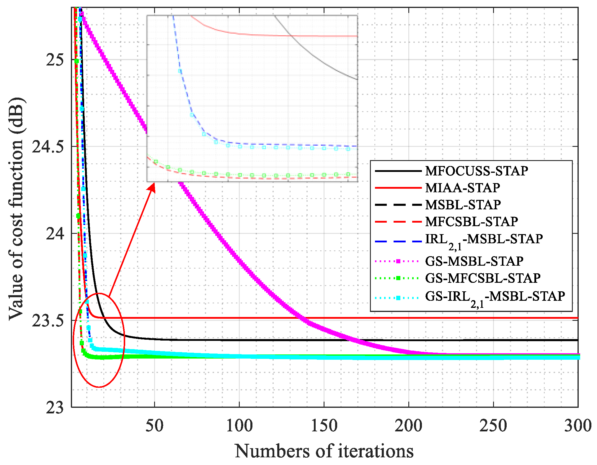
The cost function C = ln | R c + n | + Tr ( R c + n 1 R i d e a l ) can be used to evaluate the convergence performance of different SR-STAP algorithms [45]. Figure 2 plots the value of cost function versus the number of iterations curves of different SR-STAP algorithms. We find that the IR 2 , 1 - MSBL - STAP algorithm and the GS - IR 2 , 1 - MSBL - STAP algorithm converge to their steady-state values after about 12 iterations, and the MFCSBL-STAP algorithm and the GS-MFCSBL-STAP algorithm converge to their steady-state values after about 15 iterations. The MIAA-STAP algorithm and the MFOCUSS-STAP algorithm converge to their steady-state values after about 20 iterations and 50 iterations, respectively. The MSBL-STAP algorithm and the GS-MSBL-STAP algorithm converge very slowly, requiring more than 200 iterations to reach their steady-state values. We also find that the proposed computationally efficiently GS-based MSBL-STAP algorithms do not change the convergence of the original MSBL-STAP algorithms. In Table 6, the average running times of different SR-STAP algorithms are compared. The results were obtained using MATLAB 2018b and a computer with Intel(R) Xeon(R) E5-2620 CPU @ 2.40GHz 2.39 GHz. According to Figure 2, we set the number of iterations of the MFOCUSS-STAP algorithm, the MIAA-STAP algorithm, the MSBL-STAP algorithm, the MFCSBL-STAP, the IR 2 , 1 - MSBL - STAP algorithm, the GS-MSBL-STAP algorithm, the GS-MFCSBL-STAP algorithm, and the GS - IR 2 , 1 - MSBL - STAP algorithm as 50, 20, 200, 15, 12, 200, 15 and 12, respectively. From Table 6, it can be determined that the average running times of the proposed computationally efficient GS-based MSBL-STAP algorithms are far shorter than the original MSBL-STAP algorithms, thus validating the computational efficiency of our proposed algorithms.
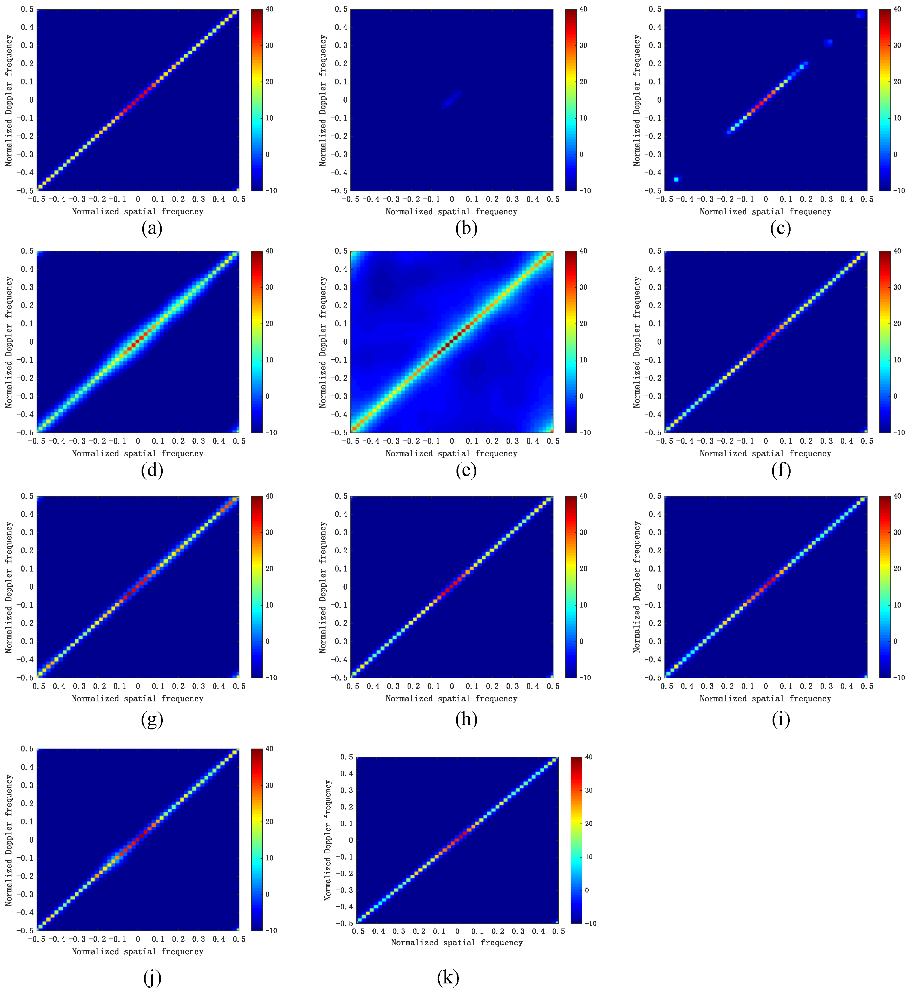
Next, we compare the clutter suppression performance of different SR-STAP algorithms. The specific simulation parameters of different SR-STAP are set as follows. The diagonal loading factor for the LSMI-STAP algorithm is 10 dB to the noise power [56]. The iteration termination thresholds of the MOMP-STAP algorithm [12], the MFOCUSS-STAP algorithm [20], the MIAA-STAP algorithm [58], the MSBL-STAP algorithm [36], the MFCSBL-STAP algorithm [45], the IR 2 , 1 - MSBL - STAP algorithm [46], the GS-MSBL-STAP algorithm, the GS-MFCSBL-STAP algorithm, and the GS - IR 2 , 1 - MSBL - STAP algorithm are all set to the same value, i.e., δ = 0.0001 . The regularization parameter for the MFOCUSS-STAP algorithm is set as p = 0.8 . Figure 3 plots the recovered clutter capon spectrums of the different SR-STAP algorithms. From Figure 3b–d, it can be observed that the clutter spectrum of the LSMI-STAP is very poor, the clutter spectrum of the MOMP-STAP is discontinuous, and the clutter spectrum of MFOCUSS-STAP has a slight spectrum expansion. The reason for this is that the CNCM cannot be well estimated using LSMI-STAP algorithms when the number of the training samples is small, and the steering vectors selected by MOMP-STAP and MFOCUSS-STAP cannot precisely span the true clutter subspace due to the limitations of the algorithm itself. From Figure 3e, it can be observed that the clutter spectrum of the MIAA-STAP has a high level of noise; this is because the space–time dictionary matrix D is not an orthogonal matrix; rather, the atoms in the space–time dictionary D are usually highly coherent. From Figure 3f–k, it can also be observed that the recovered clutter spectrums of the MSBL-STAP, the MFCSBL-STAP, the IR 2 , 1 - MSBL - STAP , the GS-MSBL-STAP, the GS-MFCSBL-STAP and the GS - IR 2 , 1 - MSBL - STAP are very close to the optimal spectrum. This shows that the MSBL-STAP algorithms can achieve superior clutter suppression performance, and the GS-based MSBL-STAP algorithms proposed by us can still achieve superior clutter suppression performance with less computational complexity.
Figure 4 depicts the SINR loss curves of different SR-STAP algorithms. All simulation results for SINR loss are averaged over 100 independent Monte Carlo trails. From Figure 4, it can be observed that the GS-MSBL-STAP algorithm, the GS-MFCSBL-STAP algorithm, and the GS - IR 2 , 1 - MSBL - STAP algorithm achieve the same performance as the MSBL-STAP algorithm, the MFCSBL-STAP algorithm, and the IR 2 , 1 - MSBL - STAP algorithm. This further indicates that the proposed computationally efficient GS-based MSBL-STAP algorithms do not change the clutter suppression performance of the original MSBL-STAP algorithms.
Then, we evaluate the target detection performance of different SR-STAP algorithms by the probability of detection probability (PD) versus SNR curves and the receive operating character (ROC) (i.e., PD versus the probability of false alarm (PFA)) curves, which are obtained by using the adaptive matched filter (AMF) detector [59]. The detection threshold and the probability of detection estimates are based on 10 4 samples. Besides, all the PD versus SNR curves and ROC curves are acquired based on 1000 independent Monte Carlo trails.
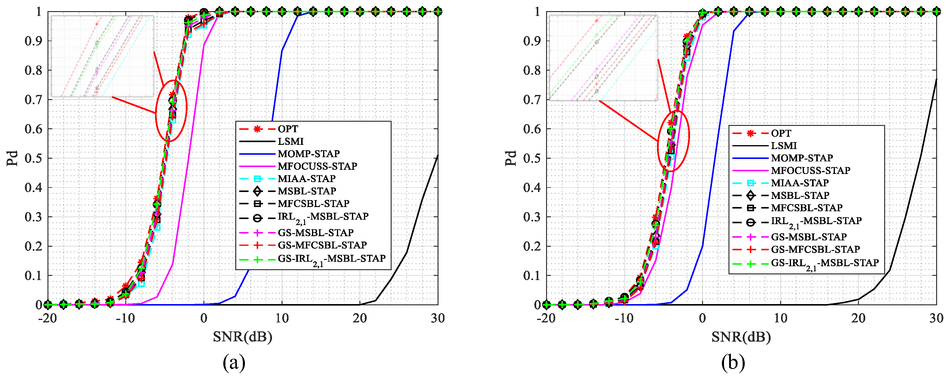
The PD versus SNR curves of different SR-STAP algorithms are depicted in Figure 5. the PFA is set as 10 3 , the target is assumed to be in the main beam direction with a Doppler frequency of 0.1 in Figure 5a and 0.3 in Figure 5b. As depicted in Figure 5a,b, the target detection performance of the MSBL-STAP algorithm, the MFCSBL-STAP, the IR 2 , 1 - MSBL - STAP algorithm, the GS-MSBL-STAP algorithm, the GS-MFCSBL-STAP algorithm, and the GS - IR 2 , 1 - MSBL - STAP algorithm are close to the optimal performance, which indicates that the MSBL-STAP algorithms have superior target detection performance whether in the mainlobe region ( f d t = 0.1 ) or in the sidelobe region ( f d t = 0.3 ). We find that the target detection performance of MIAA-STAP algorithm is slightly worse than the MSBL-STAP algorithms, the reason for this is that the recovered clutter spectrum of the MIAA-STAP has a relatively high level of noise. By comparing the PD versus SNR curves of MFCOUSS-STAP algorithm, the MOMP-STAP algorithm, and the LSMI-STAP algorithm in Figure 5a,b, we find that these algorithms have worse target detection performance in the mainlobe region ( f d t = 0.1 ), which indicates that these algorithms have poor ability to detect slow moving targets. From Figure 5a,b, it can also be observed that the GS-MSBL-STAP algorithm, the GS-MFCSBL-STAP algorithm, and the GS - IR 2 , 1 - MSBL - STAP algorithm have the same performance as the MSBL-STAP algorithm, the MFCSBL-STAP algorithm and the IR 2 , 1 - MSBL - STAP algorithm, which shows that the proposed computationally efficient GS-based MSBL-STAP algorithms do not change the target detection performance of the original MSBL-STAP algorithms.
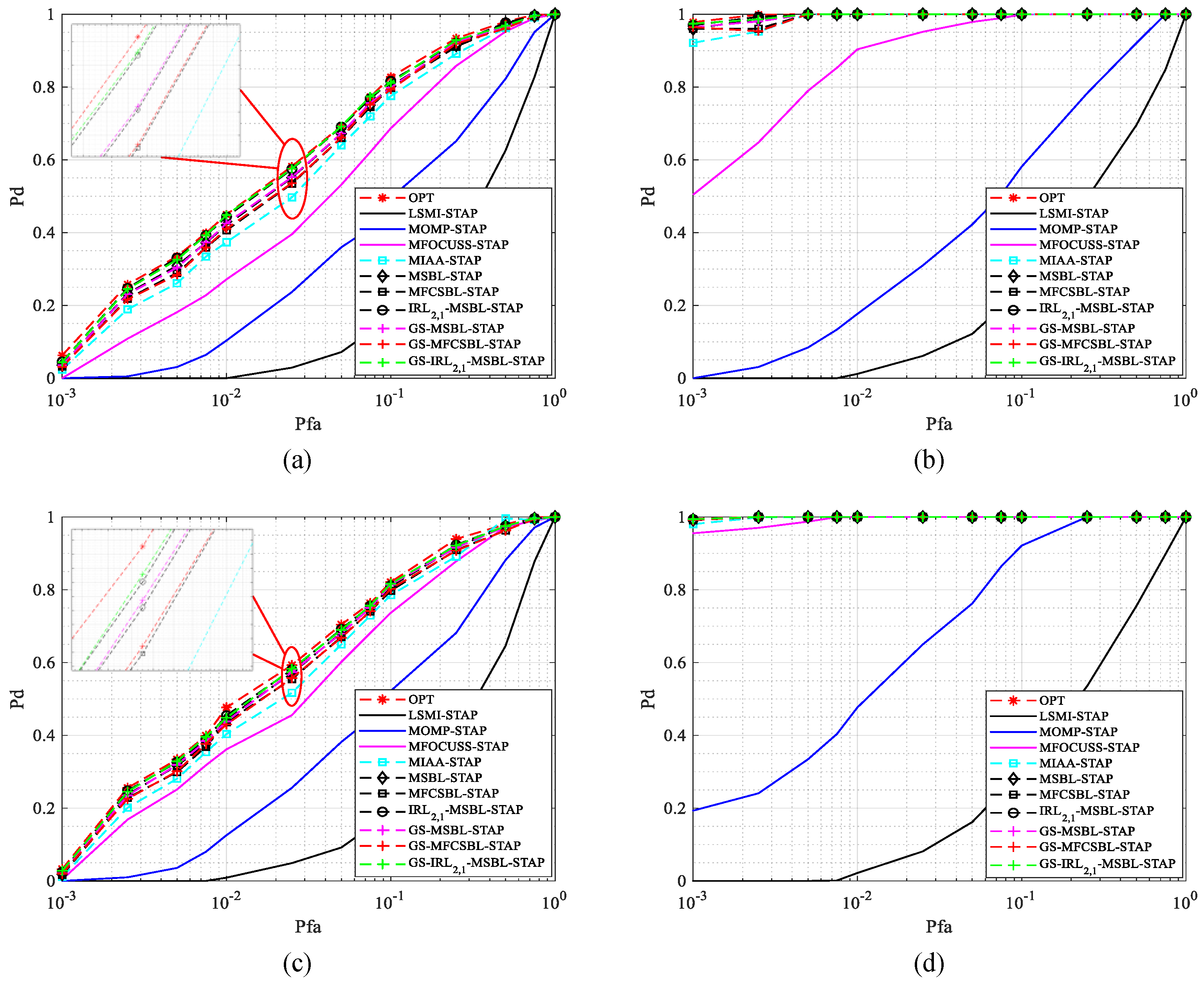
The ROC curves of different SR-STAP algorithms are depicted in Figure 6. The SNR is set as −10 dB in Figure 6a,c and −2dB in Figure 6b,d. The target is assumed to be in the main beam direction with a Doppler frequency of 0.1 in Figure 6a,b and 0.3 in Figure 6c,d. As depicted in Figure 6a–d, the MIAA-STAP algorithm, the MSBL-STAP algorithm, the MFCSBL-STAP, the IR 2 , 1 - MSBL - STAP algorithm, the GS-MSBL-STAP algorithm, the GS-MFCSBL-STAP algorithm, and the GS - IR 2 , 1 - MSBL - STAP algorithm can achieve superior target detection performance whether for fast moving targets (see Figure 6a,b) or for slow-moving targets (see Figure 6c,d). It can also be observed that the MFCOUSS-STAP algorithm, the MOMP-STAP algorithm, and the LSMI-STAP algorithm have worse target detection performance than other SR-STAP algorithms. Additionally, the target detection performance increases to various degrees with the improvement of the SNR for all SR-STAP algorithms. Similarly, it can be seen from Figure 6 that the proposed computationally efficient GS-based MSBL-STAP algorithms do not change the target performance of the original MSBL-STAP algorithms.
Figure 7 depicts the average SINR loss versus the number of training samples. As shown in Figure 7, when the number of the used training samples is greater than 6, the MSBL-STAP algorithm, the MFCSBL-STAP, the IR 2 , 1 - MSBL - STAP algorithm, the GS-MSBL-STAP algorithm, the GS-MFCSBL-STAP algorithm, and the GS - IR 2 , 1 - MSBL - STAP algorithm can achieve a near-optimal performance. For the MIAA-STAP algorithm, at least eight training samples are needed to achieve near-optimal performance. For the MFCOUSS-STAP algorithm, the MOMP-STAP algorithm, and the LSMI-STAP algorithm, more training samples are needed to achieve a steady performance.

5.2. Measured Data

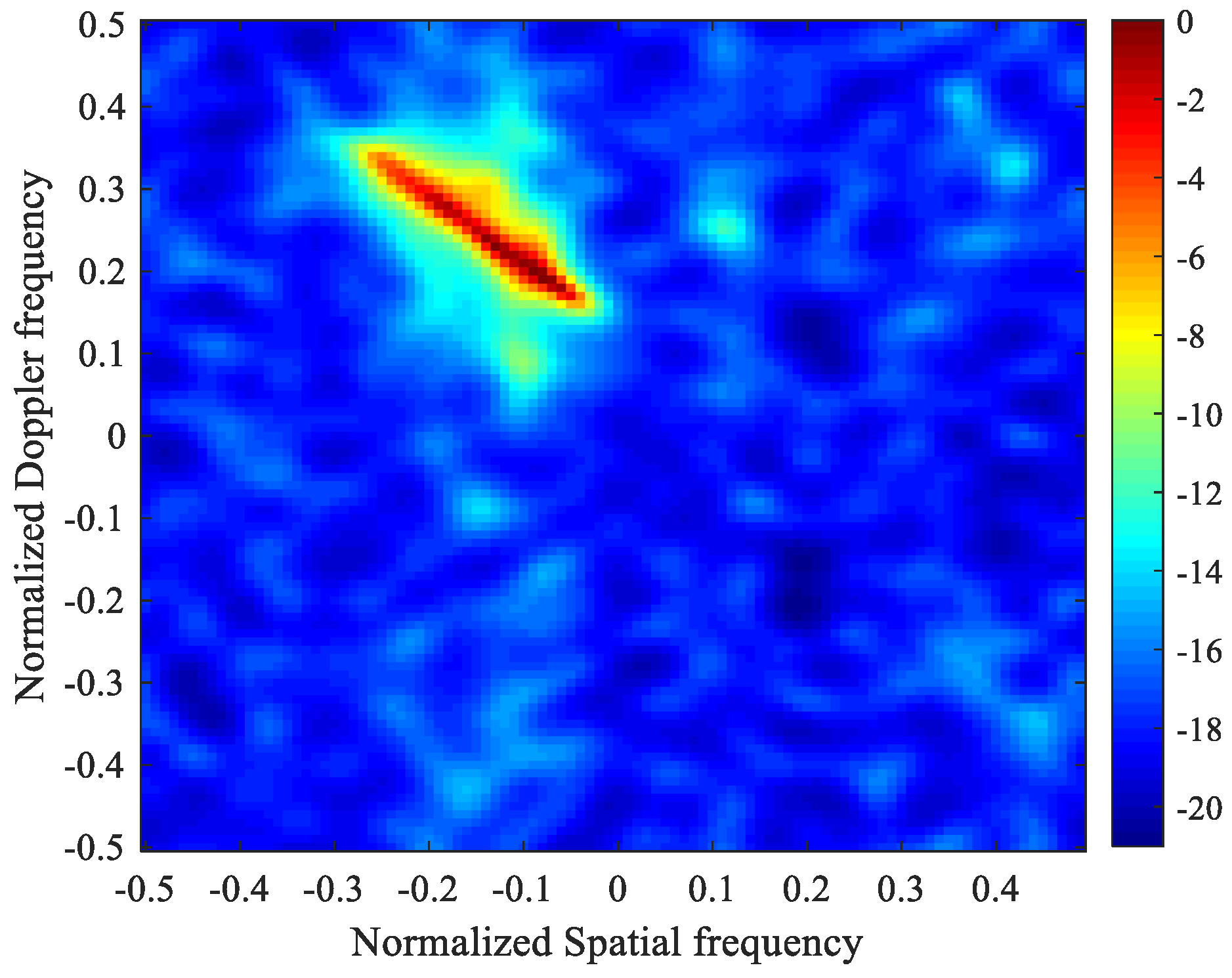
In this section, we apply the proposed GS-MSBL-STAP algorithm, the GS-MFCSBL-STAP algorithm, and the GS - IR 2 , 1 - MSBL - STAP algorithm to the publicly available Mountain-Top set, i.e., t38pre01v1 CPI6 [60]. For this data set, the received antenna array consists of 14 elements and 16 coherent pulses are transmitted in a CPI. The PRF is 625 Hz and a 500 kHz linear frequency modulated pulse is used for transmitting. There are 403 range cells in this data file and the clutter is located around 245 ° relative to true north, and the target is located at 275 ° relative to true north. The target is located in the 147th range cell, with a normalized Doppler frequency of 0.25. The estimated clutter capon spectrum using all 403 training samples is given in Figure 8. Specifically, firstly, we use all 403 range cells to estimate the clutter-plus-noise covariance matrix; then, utilizing the general formula for capon spectrum estimation, the estimated capon spectrum of the mountain-top data can be obtained. From Figure 8, it can be observed that the mountain-top data have serious heterogeneity.
Table 7 shows the average running time of different SR-STAP methods with the measured data. From Table 7, it can be observed that, compared with the original MSBL-STAP algorithms, the average running time of the proposed GS-based MSBL-STAP algorithms is significantly reduced when processing the measured data. Figure 9 depicts the STAP output for the EFA algorithm, and different SR-STAP algorithms in range cells from 130 to 165, where the curves of the MSBL-STAP algorithm, the MFCSBL-STAP algorithm, the IR 2 , 1 - MSBL - STAP algorithm are omitted, since they are visually identical to those of the GS-MSBL-STAP algorithm, the GS-MFCSBL-STAP algorithm, and the GS - IR 2 , 1 - MSBL - STAP algorithm, respectively. Ten snapshots out of 20 snapshots located next to the CUT are selected as the training data. From Figure 9, it can be observed that the target (located at 147th range cell) can be detected by all the SR-STAP algorithms even though only 10 snapshots are selected as training samples. However, since the CNCM cannot be accurately estimated, the traditional EFA algorithm cannot find the target. By comparing the STAP output of different SR-STAP algorithms, it can be observed that the proposed GS-MSBL-STAP algorithm, GS-MFCSBL-STAP algorithm, and GS - IR 2 , 1 - MSBL - STAP algorithm have better detection performance than the other SR-STAP algorithms. Moreover, since the proposed algorithms greatly reduce the computational complexity, they are more favorable for practical applications.

6. Conclusions

In this work, we developed several computationally efficient GS-based MSBL-STAP algorithms. Since the covariance matrix to be updated in the iterative process of the original MSBL-STAP algorithms is an HTBT matrix, the inverse of the covariance matrix can be decomposed using G-S factorization. Then, by exploiting the TBT/Toeplitz structural characteristics and the property whereby the space–time dictionary matrix D is the Kronecker product of two Fourier matrices, the computational complexity of the original MSBL-STAP algorithms can be significantly reduced by using the 2D-FFT/IFFT. The simulation results validate that the proposed efficient MSBL-STAP algorithms can significantly reduce the computational complexity while obtain superior clutter suppression performance and target detection performance. However, the efficient algorithms we proposed are only suitable for the case of ULA and a constant PRF with uniformly sampled spatial frequencies and Doppler frequencies. When these conditions are not met, the space–time dictionary matrix D is no longer the Kronecker product of two Fourier matrices, and the estimated covariance matrix in each iteration of the MSBL-STAP algorithms will not be an HTBT matrix; as a result, the efficient MSBL-STAP algorithms proposed in this article will no longer be applicable. Thus, in our future work, extending the proposed efficient implementation of the original MSBL-STAP algorithms under other conditions is worthy of research.

Author Contributions

Conceptualization, K.L. and T.W.; investigation, K.L. and C.L.; methodology, K.L. and J.W.; project administration, T.W.; software, K.L.; supervision, J.W.; visualization, K.L.; writing—original draft, K.L.; writing—review and editing, W.C. All authors have read and agreed to the published version of the manuscript.

Funding

This research was funded by National Key R&D Program of China, grant number 2021YFA1000400.

Conflicts of Interest

The authors declare no conflict of interest.

Appendix A

The proofs of (39)–(41) are given in Appendix A. By utilizing the property S ( K 1 ) N S ( K 1 ) N = I ( K 1 ) N , we get
R K 1 , N 1 S ( K 1 ) N = S ( K 1 ) N S ( K 1 ) N R K 1 , N 1 S ( K 1 ) N = S ( K 1 ) N R K 1 , N T = S ( K 1 ) N ( R K 1 , N H ) T = S ( K 1 ) N R K 1 , N
Substituting (38) and (39) into (35) and (36), we get
B K 1 = R K 1 , N 1 R ˜ K 1 = R K 1 , N 1 S ( K 1 ) N R K 1 S N = S ( K 1 ) N R K 1 , N R K 1 S N = S ( K 1 ) N A K 1 S N = A ˜ K 1
V N = R 0 R ˜ K 1 T R K 1 , N 1 R ˜ K 1 = R 0 S N R K 1 T S ( K 1 ) N R K 1 , N 1 S ( K 1 ) N R K 1 S N = S N S N R 0 S N S N S N R K 1 T S ( K 1 ) N R K 1 , N 1 S ( K 1 ) N R K 1 S N = S N ( S N R 0 S N R K 1 T R K 1 , N T R K 1 ) S N = S N W N T S N = W ˜ N T

Appendix B

The proofs of (56)–(58) are given in Appendix B. Given A 1 and W N ( 1 ) , according to (33) and (34), we get
A k = ( R K 1 , N 1 ) k 1 ( R K 1 ) k = { [ ( R K 1 , N 1 ) k 1 1 0 0 0 ] + [ A ˜ k 1 I N ] ( W ˜ N ( k 1 ) ) T [ A ˜ k 1 T   I N ] } [ ( R K 1 ) k 1 R k ] = [ A k 1 0 ] [ A ˜ k 1 I N ] ( W ˜ N ( k 1 ) ) T ( A ˜ k 1 T ( R K 1 ) k 1 + R k ) = [ A k 1 0 ] [ A ˜ k 1 I N ] ( W ˜ N ( k 1 ) ) T H k 1
W N ( k ) W N ( k 1 ) = ( R K 1 ) k H ( R K 1 , N 1 ) k 1 ( R K 1 ) k + ( R K 1 ) k 1 H ( R K 1 , N 1 ) k 1 1 ( R K 1 ) k 1 = ( R K 1 ) k H A k ( R K 1 ) k 1 H A k 1 = [ ( R K 1 ) k 1 H R k ] { [ A k 1 0 ] [ A ˜ k 1 I N ] ( W ˜ N ( k 1 ) ) T ( A ˜ k 1 T ( R K 1 ) k 1 + R k ) } ( R K 1 ) k 1 H A k 1 = ( ( R K 1 ) k 1 H A ˜ k 1 + R k ) ( W ˜ N ( k 1 ) ) T ( A ˜ k 1 T ( R K 1 ) k 1 + R k ) = H k 1 H ( W ˜ N ( k 1 ) ) T H k 1
W N ( k ) = W N ( k 1 ) H k 1 H ( W ˜ N ( k 1 ) ) T H k 1
where
H k 1 = A ˜ k 1 T ( R K 1 ) k 1 + R k

References

  1. Ward, J. Space-Time Adaptive Processing for Airborne Radar; MIT Lincoln Laboratory: Lexington, KY, USA, 1994. [Google Scholar]
  2. Klemm, R. Principles of Space-Time Adaptive Processing; The Institution of Electrical Engineers: London, UK, 2002. [Google Scholar]
  3. Guerci, J.R. Space-Time Adaptive Processing for Radar; Artech House: Norwood, MA, USA, 2003. [Google Scholar]
  4. Brennan, L.E.; Mallett, J.D.; Reed, I.S. Theory of Adaptive Radar. IEEE Trans. Aerosp. Electron. Syst. 1973, 9, 237–251. [Google Scholar] [CrossRef]
  5. Reed, I.S.; Mallett, J.D.; Brennan, L.E. Rapid Convergence Rate in Adaptive Arrays. IEEE Trans. Aerosp. Electron. Syst. 1974, 10, 853–863. [Google Scholar] [CrossRef]
  6. Baraniuk, R.G. Compressive sensing. IEEE Signal Proc. Mag. 2007, 24, 118–121. [Google Scholar] [CrossRef]
  7. Trzasko, J.; Manduca, A. Relaxed Conditions for Sparse Signal Recovery With General Concave Priors. IEEE Trans. Signal Process. 2009, 57, 4347–4354. [Google Scholar] [CrossRef]
  8. Davies, M.E.; Gribonval, R. Restricted Isometry Constants where ℓp sparse recovery can fail for 0 < p ≤ 1. IEEE Trans. Inf. Theory 2009, 55, 2203–2214. [Google Scholar]
  9. David, M.E.; Eldar, Y.C. Rank awareness in joint sparse recovery. IEEE Trans. Inf. Theory 2012, 58, 1135–1146. [Google Scholar]
  10. Mallat, S.G.; Zhang, Z. Matching pursuits with time-frequency dictionaries. IEEE Trans. Signal Process. 1993, 41, 3397–3415. [Google Scholar] [CrossRef]
  11. Davis, G.; Mallat, S.; Avellaneda, M. Adaptive greedy approximations. J. Constr. Approx. 1997, 13, 57–98. [Google Scholar] [CrossRef]
  12. Tropp, J.A.; Gilbert, A.C. Signal recovery from random measurements via orthogonal matching pursuit. IEEE Trans. Inf. Theory 2007, 53, 4655–4666. [Google Scholar] [CrossRef]
  13. Donoho, D.L.; Tsaig, Y.; Drori, I.; Starck, J.-L. Sparse solution of underdetermined systems of linear equations by stagewise orthogonal matching pursuit. IEEE Trans. Inf. Theory 2012, 58, 1094–1121. [Google Scholar] [CrossRef]
  14. Tropp, J.A. Just relax: Convex programming methods for identifying sparse signals in noise. IEEE Trans. Inf. Theory 2006, 52, 1030–1051. [Google Scholar] [CrossRef]
  15. Donoho, D.L.; Elad, M.; Temlyakov, V.N. Stable recovery of sparse overcomplete representations in the presence of noise. IEEE Trans. Inf. Theory 2005, 52, 6–18. [Google Scholar] [CrossRef]
  16. Koh, K.; Kim, S.J.; Boyd, S. An interior-point method for large-scale ℓ1-regularized logistic regression. J. Mach. Learn. Res. 2007, 1, 606–617. [Google Scholar]
  17. Daubechies, I.; Defrise, M.; De, M.C. An iterative thresholding algorithm for linear inverse problems with a sparsity constraint. Commun. Pure Appl. Math. J. Issued Courant Inst. Math. Sci. 2004, 57, 1413–1457. [Google Scholar] [CrossRef]
  18. Wright, S.J.; Nowak, R.D.; Figueiredo, M.A.T. Sparse reconstruction by separable approximation. IEEE Trans. Signal Process. 2009, 57, 2479–2493. [Google Scholar] [CrossRef]
  19. Donoho, D.L.; Tsaig, Y. Fast Solution of l1-Norm Minimization Problems When the Solution May Be Sparse. IEEE Trans. Inf. Theory 2008, 54, 4789–4812. [Google Scholar] [CrossRef]
  20. Gorodnitsky, I.F.; Rao, B.D. Sparse signal reconstruction from limited data using FOCUSS: A re-weighted minimum norm algorithm. IEEE Trans. Signal Process. 1997, 45, 600–616. [Google Scholar] [CrossRef]
  21. Cotter, S.; Rao, B.; Engan, K.; Kreutz-Delgado, K. Sparse solutions to linear inverse problems with multiple measurement vectors. IEEE Trans. Signal Process. 2005, 53, 2477–2488. [Google Scholar] [CrossRef]
  22. Yardibi, T.; Li, J.; Stoica, P.; Xue, M.; Baggeroer, A.B. Source localization and sensing: A nonparametric iterative adaptive approach based on weighted least squares. IEEE Trans. Aerosp. Electron. Syst. 2010, 46, 425–443. [Google Scholar] [CrossRef]
  23. Rowe, W.; Li, J.; Stoica, P. Sparse iterative adaptive approach with application to source localization. In Proceedings of the IEEE International Workshop on Computational Advances in Multi-Sensor Adaptive Processing, St. Martin, France, 15–18 December 2013; pp. 196–199. [Google Scholar]
  24. Yang, Z.C.; Li, X.; Wang, H.Q.; Jiang, W.D. On clutter sparsity analysis in space-time adaptive processing airborne radar. IEEE Geosci. Remote Sens. Lett. 2013, 10, 1214–1218. [Google Scholar] [CrossRef]
  25. Duan, K.Q.; Yuan, H.D.; Xu, H.; Liu, W.J.; Wang, Y.L. Sparisity-based non-stationary clutter suppression technique for airborne radar. IEEE Access 2018, 6, 56162–56169. [Google Scholar] [CrossRef]
  26. Yang, Z.C.; Wang, Z.T.; Liu, W.J. Reduced-dimension space-time adaptive processing with sparse constraints on beam-Doppler selection. Signal Process. 2019, 157, 78–87. [Google Scholar] [CrossRef]
  27. Zhang, W.; An, R.X.; He, Z.S.; Li, H.Y. Reduced dimension STAP based on sparse recovery in heterogeneous clutter environments. IEEE Trans. Aerosp. Electron. Syst. 2020, 56, 785–795. [Google Scholar] [CrossRef]
  28. Li, Z.Y.; Wang, T. ADMM-Based Low-Complexity Off-Grid Space-Time Adaptive Processing Methods. IEEE Access 2020, 8, 206646–206658. [Google Scholar] [CrossRef]
  29. Su, Y.Y.; Wang, T.; Li, Z.Y. A Grid-Less Total Variation Minimization-Based Space-Time Adaptive Processing for Airborne Radar. IEEE Access 2020, 8, 29334–29343. [Google Scholar] [CrossRef]
  30. Tipping, M.E. Sparse Bayesian learning and the relevance vector machine. J. Mach. Learn. 2001, 1, 211–244. [Google Scholar]
  31. Wipf, D.P.; Rao, B.D. Sparse Bayesian learning for basis selection. IEEE Trans. Signal Process. 2004, 52, 2153–2164. [Google Scholar] [CrossRef]
  32. Wipf, D.P.; Rao, B.D. An empirical Bayesian strategy for solving the simultaneous sparse approximation problem. IEEE Trans. Signal Process. 2007, 55, 3704–3716. [Google Scholar] [CrossRef]
  33. Ji, S.; Xue, Y.; Carin, L. Bayesian compressive sensing. IEEE Trans. Signal Process. 2008, 56, 2346–2356. [Google Scholar] [CrossRef]
  34. Baraniuk, R.G.; Cevher, V.; Duarte, M.F.; Hegde, C. Model-based compressive sensing. IEEE Trans. Inf. Theory 2010, 56, 1982–2001. [Google Scholar] [CrossRef]
  35. Zhang, Z.; Rao, B.D. Extension of SBL algorithms for the recovery of block sparse signals with intra-block correlation. IEEE Trans. Signal Process. 2013, 61, 2009–2015. [Google Scholar] [CrossRef]
  36. Duan, K.Q.; Wang, Z.T.; Xie, W.C.; Chen, H.; Wang, Y.L. Sparsity-based STAP algorithm with multiple measurement vectors via sparse Bayesian learning strategy for airborne radar. IET Signal Process. 2017, 11, 544–553. [Google Scholar] [CrossRef]
  37. Sun, Y.; Yang, X.; Long, T.; Sarkar, T.K. Robust sparse Bayesian learning STAP method for discrete interference suppression in nonhomogeneous clutter. In Proceedings of the IEEE Radar Conference, Seattle, WA, USA, 8–12 May 2017; pp. 1003–1008. [Google Scholar]
  38. Wu, Q.; Zhang, Y.D.; Amin, M.G.; Himed, B. Space-Time Adaptive Processing and Motion Parameter Estimation in Multistatic Passive Radar Using Sparse Bayesian Learning. IEEE Trans. Geosci. Remote Sens. 2016, 54, 944–957. [Google Scholar] [CrossRef]
  39. Li, Z.H.; Guo, Y.D.; Zhang, Y.S.; Zhou, H.; Zheng, G.M. Sparse Bayesian learning based space-time adaptive processing against unknown mutual coupling for airborne radar using middle subarray. IEEE Access 2019, 7, 6094–6108. [Google Scholar] [CrossRef]
  40. Liu, H.; Zhang, Y.; Guo, Y.; Wang, Q.; Wu, Y. A novel STAP algorithm for airborne MIMO radar based on temporally correlated multiple sparse Bayesian learning. Math. Probl. Eng. 2016, 2016, 3986903. [Google Scholar] [CrossRef]
  41. Liu, C.; Wang, T.; Zhang, S.; Ren, B. A Fast Space-Time Adaptive Processing Algorithm Based on Sparse Bayesian Learning for Airborne Radar. Sensors 2022, 22, 2664. [Google Scholar] [CrossRef]
  42. Liu, K.; Wang, T.; Wu, J.; Chen, J. A Two-Stage STAP Method Based on Fine Doppler Localization and Sparse Bayesian Learning in the Presence of Arbitrary Array Errors. Sensors 2022, 22, 77. [Google Scholar] [CrossRef]
  43. Cui, N.; Xing, K.; Duan, K.; Yu, Z. Knowledge-aided block sparse Bayesian learning STAP for phased-array MIMO airborne radar. IET Radar Sonar Navig. 2021, 15, 1628–1642. [Google Scholar] [CrossRef]
  44. Cui, N.; Xing, K.; Duan, K.; Yu, Z. Fast Tensor-based Three-dimensional Sparse Bayesian Learning Space-Time Adaptive Processing Method. J. Radars 2021, 10, 919–928. [Google Scholar]
  45. Wang, Z.T.; Xie, W.; Duan, K.; Wang, Y. Clutter suppression algorithm based on fast converging sparse Bayesian learning for airborne radar. Signal Process. 2017, 130, 159–168. [Google Scholar] [CrossRef]
  46. Liu, C.; Wang, T.; Zhang, S.; Ren, B. Clutter suppression based on iterative reweighted methods with multiple measurement vectors for airborne radar. IET Radar Sonar Navig. 2022; early view. [Google Scholar] [CrossRef]
  47. Xue, M.; Xu, L.; Li, J. IAA spectral estimation: Fast implementation using the Gohberg–Semencul factorization. IEEE Trans. Signal Process. 2011, 59, 3251–3261. [Google Scholar]
  48. Kailath, T.; Sayed, A.H. Displacement structure: Theory and applications. SIAM Rev. 1995, 37, 297–386. [Google Scholar] [CrossRef]
  49. Blahut, R.E. Fast Algorithms for Signal Processing; Cambridge University Press: London, UK, 2010. [Google Scholar]
  50. Noor, F.; Morgera, S.D. Recursive and iterative algorithms for computing eigenvalues of Hermitian Toeplitz matrices. IEEE Trans. Signal Process. 1993, 41, 1272–1280. [Google Scholar] [CrossRef]
  51. Jain, J.R. An efficient algorithm for a large Toeplitz set of linear equations. IEEE Trans. Acoust. Speech Signal Process. 1980, 27, 612–615. [Google Scholar] [CrossRef]
  52. Glentis, G.O.; Jakobsson, A. Efficient implementation of iterative adaptive approach spectral estimation techniques. IEEE Trans. Signal Process. 2011, 59, 4154–4167. [Google Scholar] [CrossRef]
  53. Harville, D.A. Matrix Algebra from a Statistician’s Perspective; Springer: New York, NY, USA, 1998. [Google Scholar]
  54. Wax, M.; Kailath, T. Efficient inversion of Toeplitz-block Toeplitz matrix. IEEE Trans. Acoust. Speech Signal Process. 1983, 31, 1218–1221. [Google Scholar] [CrossRef]
  55. Musicus, B. Fast MLM power spectrum estimation from uniformly spaced correlations. IEEE Trans. Acoust. Speech Signal Process. 1985, 33, 333–1335. [Google Scholar] [CrossRef]
  56. Glentis, G.O. A Fast Algorithm for APES and Capon Spectral Estimation. IEEE Trans. Signal Process. 2008, 56, 4207–4220. [Google Scholar] [CrossRef]
  57. Jakobsson, A.; Marple, S.L.; Stoica, P. Computationally efficient two-dimensional Capon spectrum analysis. IEEE Trans. Signal Process. 2000, 48, 2651–2661. [Google Scholar] [CrossRef]
  58. Yang, Z.; Li, X.; Wang, H.; Jiang, W. Adaptive clutter suppression based on iterative adaptive approach for airborne radar. Signal Process. 2013, 93, 3567–3577. [Google Scholar] [CrossRef]
  59. Robey, F.; Fuhrmann, D.; Kelly, E.; Nitzberg, R. A CFAR adaptive matched filter detector. IEEE Trans. Aerosp. Electron. Syst. 1992, 28, 208–216. [Google Scholar] [CrossRef]
  60. Titi, G.W.; Marshall, D.F. The ARPA/NAVY Mountaintop Program: Adaptive signal processing for airborne early warning radar. In Proceedings of the 1996 IEEE International Conference on Acoustics, Speech, and Signal Processing, Atlanta, GA, USA, 9 May 1996. [Google Scholar]
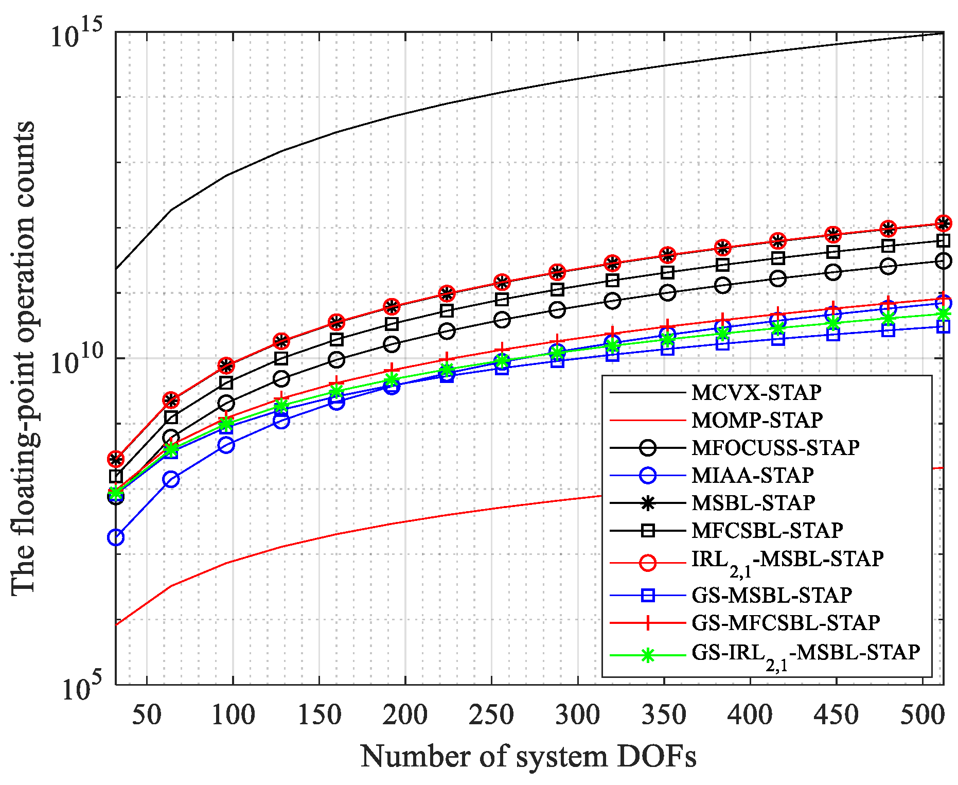
Figure 1. Computational complexities of different SR-STAP algorithms.
Remotesensing 14 03931 g001
Figure 2. Value of cost function versus the number of iterations.
Remotesensing 14 03931 g002
Figure 3. Clutter capon spectrums of different SR-STAP algorithms. (a) OPT; (b) LSMI-STAP; (c) MOMP-STAP; (d) MFCOUSS-STAP; (e) MIAA-STAP; (f) MSBL-STAP; (g) MFCSBL-STAP; (h) IR 2 , 1 - MSBL - STAP ; (i) GS-MSBL-STAP; (j) GS-MFCSBL-STAP; (k) GS - IR 2 , 1 - MSBL - STAP .
Remotesensing 14 03931 g003
Figure 4. SINR loss comparison of different SR-STAP algorithms.
Remotesensing 14 03931 g004
Figure 5. PD versus SNR curves of different SR-STAP algorithms. (a) the normalized target Doppler frequency f d t = 0.1 ; (b) the normalized target Doppler frequency f d t = 0.3 .
Remotesensing 14 03931 g005
Figure 6. ROC curves of different SR-STAP algorithms. (a) f d t = 0 . 1 , SNR = 10   dB ; (b) f d t = 0 . 1 , SNR = 2   dB ; (c) f d t = 0 . 3 , SNR = 10   dB ; (d) f d t = 0 . 3 , SNR = 2   dB .
Remotesensing 14 03931 g006
Figure 7. Average SINR loss versus the number of training samples.
Remotesensing 14 03931 g007
Figure 8. Estimated clutter capon spectrum with all 403 samples.
Remotesensing 14 03931 g008
Figure 9. STAP output power against the range cell for different algorithms.
Remotesensing 14 03931 g009
Table 1. Pseudocode of MFCSBL-STAP algorithm.
Input: training samples Y , dictionary matrix D .
Initialize:
    γ 0 = 1 , ( σ 0 2 ) 0 = 1 , Γ 0 = d i a g ( γ 0 ) , R 0 = ( σ 2 ) 0 I N K + D Γ 0 D H , R ML = Y Y H / L .
Repeat:
    μ t = Γ t D H ( R t ) 1 Y
    γ m t + 1 = ( γ m t ) 2 | v m H ( R t ) 1 R ML ( R t ) 1 v m | ,   ( m = 1 , 2 , , N s K d )
    ( σ 2 ) t + 1 = ( 1 / L ) Y D μ t F 2 / [ N K m = 1 N s K d γ m t v m H ( R t ) 1 v m ]   ( m = 1 , 2 , , N s K d )
    R t + 1 = ( σ 2 ) t + 1 I N K + D Γ t + 1 D H
The iterative procedure terminates when the iteration termination condition in (12) is satisfied.
Get the estimated angle-Doppler profile X ^ using (13).
Reconstruct the CNCM using (14) and compute the optimal STAP weight vector using (15).
Table 2. Pseudocode of IR 2 , 1 - MSBL - STAP algorithm.
Input: training samples Y , dictionary matrix D .
Initialize:
    γ 0 = 1 , ( σ 0 2 ) 0 = 1 , Γ 0 = d i a g ( γ 0 ) , R 0 = ( σ 2 ) 0 I N K + D Γ 0 D H .
Repeat:
    μ t = Γ t D H ( R t ) 1 Y
    Σ t = Γ t Γ t D H ( R t ) 1 D Γ t
    γ m t + 1 = [ v m H ( R t ) 1 v m ] 1 2 [ 1 L l = 1 L ( μ l , m t ) 2 ] 1 2 ,   ( m = 1 , 2 , , N s K d )
    ( σ 2 ) t + 1 = [ ( 1 / L ) Y D μ t F 2 ] / ( N K m = 1 N s K d ( 1 Σ m , m t / γ m t ) )   ( m = 1 , 2 , , N s K d )
    R t + 1 = ( σ 2 ) t + 1 I N K + D Γ t + 1 D H
The iterative procedure terminates when the iteration termination condition in (12) is satisfied.
Get the estimated angle-Doppler profile X ^ using (13).
Reconstruct the CNCM using (14) and compute the optimal STAP weight vector using (15).
Table 3. Simulation parameters of the radar system.
ParameterValue
Bandwidth2.5 M
Wavelength0.3 m
Pulse repetition frequency2000 Hz
Platform velocity150 m/s
Platform height9 km
Element number8
Pulse number8
CNR40 dB
Table 4. Computational complexity comparison.
AlgorithmThe Number of Floating-Point Operations for a Single Iteration
MCVX-STAP o ( 8 ( N s K d L ) 3 )
MOMP-STAP o ( 8 N K N s K d L + 8 r s 3 + 16 N K r s 2 + 8 N K L r s )
MFOCUSS-STAP o ( 8 N K N s K d L + 8 ( N K ) 3 + 8 N K ( N s K d ) 2 + 16 ( N K ) 2 N s K d )
MIAA-STAP o ( 8 N K N s K d L + 8 ( N K ) 3 + 32 ( N K ) 2 N s K d + 16 N K N s K d )
MSBL-STAP o ( 8 N K N s K d L + 8 ( N K ) 3 + 32 N K ( N s K d ) 2 + 24 ( N K ) 2 N s K d )
MFCSBL-STAP o ( 8 N K N s K d L + 8 ( N K ) 3 + 16 N K ( N s K d ) 2 + 40 ( N K ) 2 ( N s K d ) )
IR 2 , 1 - MSBL - STAP o ( 8 N K N s K d L + 8 ( N K ) 3 + 32 N K ( N s K d ) 2 + 32 ( N K ) 2 N s K d )
GS-MSBL-STAP o ( 8 N 3 ( K 2 K + 2 ) + 5 ( L + 1 ) N s K d log 2 ( N s K d ) + 5 ( N K ) 2 log 2 ( N K ) + 8 N s K d N K L )
GS-MFCSBL-STAP o ( 8 N 3 ( K 2 K + 2 ) + 5 ( L + 1 ) N s K d log 2 ( N s K d ) + 8 N K N s K d L + 24 ( N K ) 2 N s K d )
GS - IR 2 , 1 - MSBL - STAP o ( 8 N 3 ( K 2 K + 2 ) + 5 ( L + 1 ) N s K d log 2 ( N s K d ) + 5 ( N K ) 2 log 2 ( N K ) + 8 N K N s K d L + 8 ( N K ) 2 N s K d )
Table 5. Computational complexities of various SR-STAP algorithms under different system DOFs.
System DOFs128256512
The Number of
Floating-Operations for
Single Iteration
Algorithm
MCVX-STAP1.484 × 10131.187 × 10149.499 × 1014
MOMP-STAP1.296 × 1075.206 × 1072.111 × 108
MFOCUSS-STAP4.861 × 1093.884 × 10103.105 × 1011
MIAA-STAP1.107 × 1098.791 × 1097.006 × 1010
MSBL-STAP1.802 × 10101.441 × 10111.152 × 1012
MFCSBL-STAP9.962 × 1097.964 × 10106.369 × 1011
IR 2 , 1 - MSBL - STAP 1.828 × 10101.462 × 10111.169 × 1012
GS-MSBL-STAP1.619 × 1097.072 × 1093.070 × 1010
GS-MFCSBL-STAP2.424 × 1091.351 × 10108.223 × 1010
GS - IR 2 , 1 - MSBL - STAP 1.888 × 1099.220 × 1094.788 × 1010
Table 6. Average running time comparison.
AlgorithmRunning Time
MCVX-STAP900.4931 s
MOMP-STAP0.0254 s
MFOCUSS-STAP3.8556 s
MIAA-STAP0.7614 s
MSBL-STAP15.1402 s
MFCSBL-STAP1.4835 s
IR 2 , 1 - MSBL - STAP 1.8533 s
GS-MSBL-STAP1.3409 s
GS-MFCSBL-STAP0.3610 s
GS - IR 2 , 1 - MSBL - STAP 0.1914 s
Table 7. Average running time of different SR-STAP methods with measured data.
AlgorithmRunning Time
MFOCUSS-STAP41.9740 s
MIAA-STAP2.3135 s
MSBL-STAP43.8430 s
MFCSBL-STAP4.7761 s
IR 2 , 1 - MSBL - STAP 6.7693 s
GS-MSBL-STAP2.3971 s
GS-MFCSBL-STAP0.8380 s
GS - IR 2 , 1 - MSBL - STAP 0.4277 s
Publisher’s Note: MDPI stays neutral with regard to jurisdictional claims in published maps and institutional affiliations.