Improved Dimension-Reduced Structures of 3D-STAP on Nonstationary Clutter Suppression for Space-Based Early Warning Radar

Abstract

By introducing degrees of freedom (DOFs) in elevation, the elevation-azimuth-Doppler three-dimensional space–time adaptive processing (3D-STAP) methods have better performance when suppressing the nonstationary clutter caused by the Earth’s rotation in space-based early warning radar (SBEWR). However, the 3D-STAP methods use much more auxiliary beams, leading to greater demands on the training samples and heavier computational burdens than the conventional STAP methods. To solve this problem, the ideas of sum–difference beams, generalized multiple beams and Doppler-domain localization are applied here, and three improved dimension-reduced structures of 3D-STAP are proposed in this article. After analyzing the characteristics and distribution of nonstationary clutter for SBEWR, we find that the demands for auxiliary beams are different in elevation, azimuth and Doppler dimension. In addition, the suggestion to choose the number of auxiliary beams in each dimension is given. Simulation experiments are conducted to verify the analysis and evaluate the performance of the proposed methods. The simulation results show that the proposed 3D-STAP methods have better performance and lower computational burdens than typical 3D-STAP methods.

1. Introduction

Space-based early warning radar (SBEWR), located on satellites, can provide a larger detection range and a longer early warning time than airborne early warning radar (AEWR) due to its higher orbit height and ability to carry out global observation. Restricted by the curvature of the Earth, SBEWR should be mainly focused downward. However, there will be strong interference of the ground clutter when detecting moving targets. Therefore, clutter suppression plays an important role in moving target detection [1,2,3]. Further, the Earth’s rotation [4] makes the clutter nonstationary, which means that the clutter from different range gates have different space–time distributions. In addition, SBEWR usually works at a medium or high pulse repetition frequency (PRF) with a much larger detection range, which causes range ambiguity (RA). Severe RA degrades the performance of the conventional two-dimensional space–time adaptive processing (2D-STAP) methods [5,6,7,8] on non-stationary clutter suppression.

At present, few methods have been proposed to solve the problem of the nonstationary clutter suppression in SBEWR. The main methods developed for non-stationary clutter suppression have been proposed for AEWR. These methods can be used as references for SBEWR and can be divided into three types, compensation methods [9,10,11,12], elevation adaptive filter (EAF) methods [13,14,15] and 3D-STAP methods [16,17]. Firstly, in terms of compensation methods, the main idea is to compensate for the phase differences between each range gate so that the clutter from different range gates has the same space–time distribution. Typical compensation methods include the Doppler Warping (DW) [9], Angle-Doppler compensation (ADC) [10], adaptive Angle-Doppler compensation (A²DC) [11] and Registration-Based compensation (RBC) [12]. These compensation methods can be used in the absence of RA. Once there is RA, the phase compensations of the near-range RA components will aggravate the non-stationarity of the far-range RA components. Therefore, the compensation methods are not suitable for SBEWR which has many range ambiguities. EAF methods include Elevation Robust Capon Beamforming (ERCB) [13], Elevation Sum and Difference Beamforming (ESDB) [14], Subspace Projection prefiltering (SPP) [15] and so on. The main idea is to use the statistical regularity with which the clutter in different RA components has different elevation angles to form several nulls at the positions of each RA component. Then conventional 2D-STAP methods are used for the residual stationary clutter suppression. However, the number of RAs is usually much greater than the number of array elements in the elevation dimension for SBEWR due to the limitation of the antenna size and the severe RAs. Therefore, compared with AEWR, the performance of EAF methods on the non-stationary clutter suppression in SBEWR is degraded. Finally, the main idea of 3D-STAP is to use the elevation-azimuth-Doppler three-dimensional information of the clutter to estimate the clutter covariance matrix (CCM) and perform an adaptive filter. Typical 3D-STAP methods include 3D-Joint Domain Localization (3D-JDL) [16] and 3D-Subarray Synthesis (3D-SS) STAP [17]. Due to the addition of the elevation dimension as compared to 2D-STAP without this dimension, 3D-STAP methods can achieve good performance on non-stationary clutter suppression. However, the use of the elevation dimension causes the number of auxiliary beams to increase rapidly. On the one hand, the increase in auxiliary beams will make greater demands on the training samples in order to meet the Reed–Mallet–Brennan (RMB) rule [18]. On the other hand, the increase in auxiliary beams will also cause a much larger CCM, which will lead to much heavier computational burdens.

Aiming to solve the abovementioned problems with 3D-STAP, three improved dimension-reduced structures of 3D-STAP are proposed to reduce the total number of auxiliary beams. First, the 3D distributions of the nonstationary clutter are analyzed for SBEWR. The characteristic differences in the nonstationary clutter between SBEWR and AEWR are compared. Then, by applying the ideas of sum and difference beams (SDB), generalized multiple beams (GMB) and Doppler-domain localization (DDL) to 3D-STAP, three improved dimension-reduced structures of 3D-STAP are proposed. The regularity is discussed and is found to indicate the relative relationships of the required auxiliary beams for the three dimensions. Finally, simulation experiments are conducted to analyze the performance of the proposed 3D-STAP methods. The results of the experiments verify that the proposed 3D-STAP methods have a better performance on the nonstationary clutter suppression in SBEWR than the previous methods, and the total number of auxiliary beams is smaller.

2. Signal Model and Conventional 3D-STAP Methods

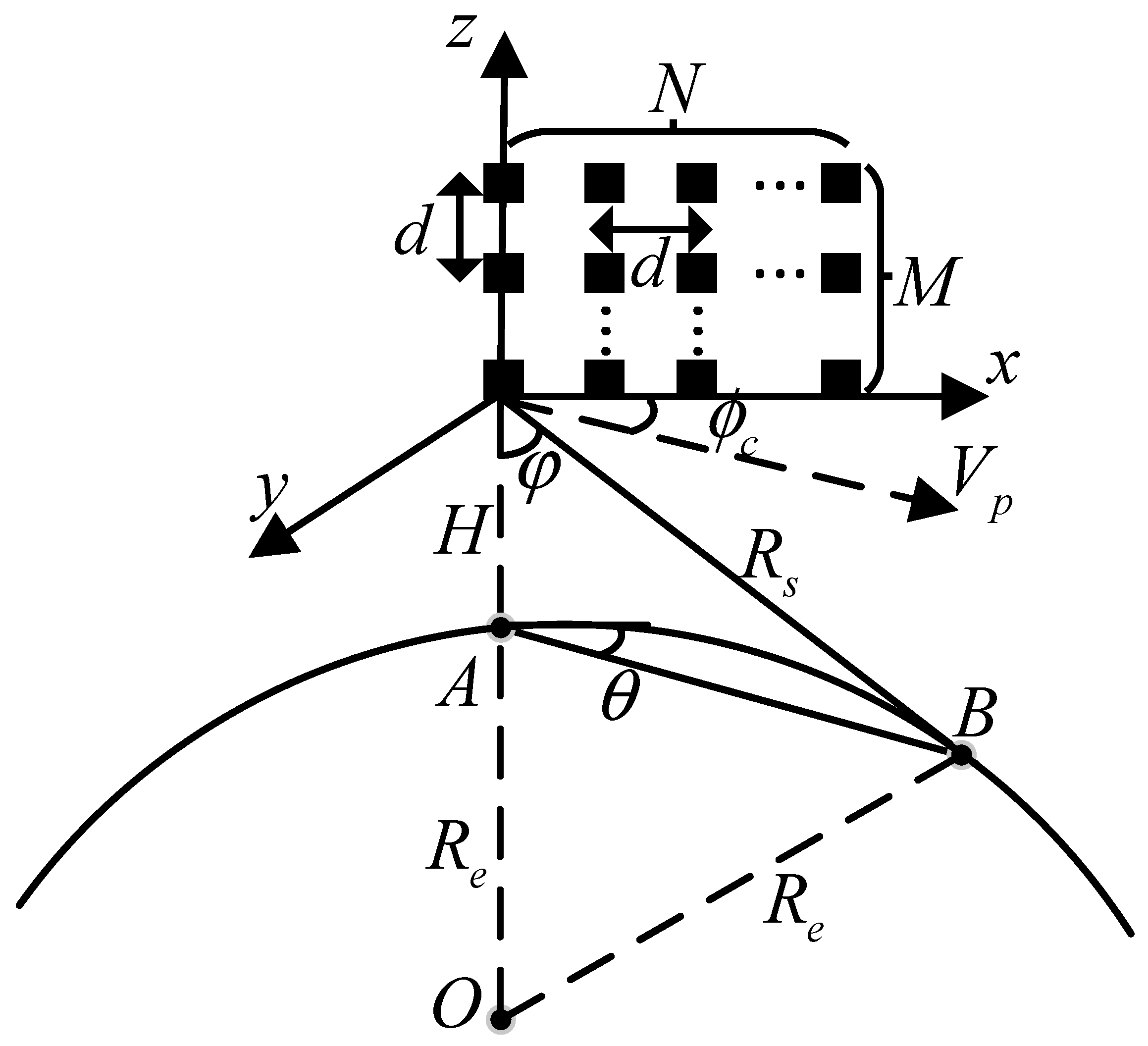
2.1. Signal Model for SBEWR

The observation geometry of SBEWR is shown in Figure 1. Points O, A and $R_e$ denote the geocenter, nadir point and the radius of the Earth, respectively. The satellite flies at the orbit height of $H$ with the speed of $V_p$. SBEWR illustrates point B on the ground at the slant range of $R_s$, with an elevation angle of $\phi$ and azimuth angle of $\theta$. The 2D antenna array is formed of $M$ elements in the elevation dimension and $N$ elements in the azimuth with the array interval of $d$. The antenna array is placed in the direction of the x-axis.

The frequency of clutter in the elevation, azimuth and Doppler domain can be expressed, respectively, as

$$f_{se}=\frac{d}{\lambda }\cos \phi$$

(1)

$$f_{sa}=\frac{d}{\lambda }\cos \psi =\frac{d}{\lambda }\sin \phi \cos \theta$$

(2)

$$f_d=\frac{2V_p}{\lambda f_r}{\rho }_c\sin \phi \cos \left(\theta +{\varphi }_c\right)$$

(3)

where $\lambda$ and $f_r$ denote the wavelength and PRF, respectively. $\psi$ is the cone angle. ${\rho }_c$ and ${\varphi }_c$ are the crab magnitude and crab angle caused by the Earth’s rotation, respectively, which can be expressed as [19]

$${\rho }_c=\sqrt{1+{\mathrm{\Delta }}^2{\cos }^2\alpha -2\mathrm{\Delta }\cos \eta }$$

(4)

$${\varphi }_c=\arctan \left(\frac{\mathrm{\Delta }\sqrt{{\cos }^2\alpha -{\cos }^2\eta }}{1-\mathrm{\Delta }\cos \eta }\right)$$

(5)

where $\alpha$ and $\eta$ denote the latitude of point A and the orbit inclination angle of the satellite, respectively. $\mathrm{\Delta }=V_e/V_p\left(1+H/R_e\right)$ where $V_e$ is the velocity of the Earth’s rotation over the equator. The steering vectors of clutter in the elevation, azimuth and Doppler dimensions can be formulated, respectively, as

$$V_{se}\left(f_{se}\right)={\left[1,\exp \left(j2\pi f_{se}\right),\cdots ,\exp \left(j2\pi \left(M-1\right)f_{se}\right)\right]}^T\in {ℂ}^{M\times 1}$$

(6)

$$V_{sa}\left(f_{sa}\right)={\left[1,\exp \left(j2\pi f_{sa}\right),\cdots ,\exp \left(j2\pi \left(N-1\right)f_{sa}\right)\right]}^T\in {ℂ}^{N\times 1}$$

(7)

$$V_d\left(f_d\right)={\left[1,\exp \left(j2\pi f_d\right),\cdots ,\exp \left(j2\pi \left(K-1\right)f_d\right)\right]}^T\in {ℂ}^{K\times 1}$$

(8)

where ${\left(\cdot \right)}^T$ denotes the transpose of a matrix. $K$ is the number of pulses in a coherent pulse interval (CPI). Then the 3D steering vector of clutter can be expressed as

$$V_{3\mathrm{D}}=V_{se}\left(f_{se}\right)\otimes V_{sa}\left(f_{sa}\right)\otimes V_d\left(f_d\right)\in {ℂ}^{MNK\times 1}$$

(9)

Therefore, the 3D signal model of the clutter in the $l$-th range gate can be formulated as

$$X_l={\displaystyle \sum _{p=1}^{N_R}{\displaystyle \sum _{q=1}^{N_c}{\sigma }_{l,p,q}\cdot V_{3\mathrm{D}}\left(l,p,q\right)}},\hspace{1em}l=1~L$$

(10)

where $N_R$ and $N_c$ denote the number of range ambiguities and statistical independent clutter patches within a range bin, respectively; $\sigma$ is the corresponding amplitude of the clutter patch; $\otimes$ denotes the Kronecker product operation. Then the echo of the $l$-th range gate for the SBEWR in the presence of targets can be formulated as

$$X=X_l+X_t+X_n$$

(11)

where $X_n$ is the signal of noise which is assumed to be Gaussian white noise. $X_t$ is the signal of targets. It can be seen that clutter suppression is a key point for moving targets detection.

2.2. A Brief Review on Conventional 3D-STAP Methods

First, two typical 3D-STAP methods, which are 3D-JDL and 3D-SS, are introduced here. In terms of reducing dimension in different domains, 3D-JDL is a typical beam-space post-Doppler STAP method, which uses the conventional beamforming to transform the pulse signal into the Doppler domain and array signal into beam-space for dimension reduction and STAP afterwards. In addition, 3D-SS belongs to element–space pre-Doppler STAP methods, which performs dimension reduction by subarray synthesis and STAP in time domain and element–space directly. The dimension-reduced matrix of 3D-JDL can be formulated as [16]

$$T_{3\mathrm{DJDL}}=T_{\mathrm{JDL},\mathrm{el}}\otimes T_{\mathrm{JDL},\mathrm{az}}\otimes T_{\mathrm{JDL},\mathrm{d}}$$

(12)

The dimension-reduced matrix of each dimension can be expressed, respectively, as

$$T_{\mathrm{JDL},\mathrm{el}}=\left[V_{se}\left(f_{se}\left(t-m\right)\right),\cdots ,V_{se}\left(f_{se}\left(t\right)\right),\cdots ,V_{se}\left(f_{se}\left(t+m\right)\right)\right]\in {ℂ}^{M\times \left(2m+1\right)}$$

(13)

$$T_{\mathrm{JDL},\mathrm{az}}=\left[V_{sa}\left(f_{sa}\left(t-n\right)\right),\cdots ,V_{sa}\left(f_{sa}\left(t\right)\right),\cdots ,V_{sa}\left(f_{sa}\left(t+n\right)\right)\right]\in {ℂ}^{N\times \left(2n+1\right)}$$

(14)

$$T_{\mathrm{JDL},\mathrm{d}}=\left[V_d\left(f_d\left(t-k\right)\right),\cdots ,V_d\left(f_d\left(t\right)\right),\cdots ,V_d\left(f_d\left(t+k\right)\right)\right]\in {ℂ}^{K\times \left(2k+1\right)}$$

(15)

where $f_{se}\left(t\right)$, $f_{sa}\left(t\right)$ and $f_d\left(t\right)$ denote the frequency of the target in the elevation, azimuth and Doppler dimensions, respectively. The number of auxiliary beams in elevation, azimuth and Doppler are 2m + 1, 2n + 1 and 2k + 1, respectively.

The dimension-reduced matrix of 3D-SS can be expressed as [17]

$$T_{3\mathrm{DSS}}=T_{3\mathrm{DSS},\mathrm{S}}\otimes I_K$$

(16)

where $I_K$ is a $K\times K$ identity matrix. The spatial dimension-reduced matrix can be detailed as

$$T_{3\mathrm{DSS},\mathrm{S}}=\left[T_{3\mathrm{DSS},\mathrm{se}},T_{3\mathrm{DSS},\mathrm{sa}}\right]$$

(17)

$$T_{3\mathrm{DSS},\mathrm{se}}=\left[V_{se}\left(f_{se}\left(t\right)\right)\otimes g_1,\cdots ,V_{se}\left(f_{se}\left(t\right)\right)\otimes g_n,\cdots ,V_{se}\left(f_{se}\left(t\right)\right)\otimes g_N\right]\in {ℂ}^{MN\times N}$$

(18)

$$T_{3\mathrm{DSS},\mathrm{sa}}=\left[g_1\otimes V_{sa}\left(f_{sa}\left(t\right)\right),\cdots ,g_n\otimes V_{sa}\left(f_{sa}\left(t\right)\right),\cdots ,g_N\otimes V_{sa}\left(f_{sa}\left(t\right)\right)\right]\in {ℂ}^{MN\times M}$$

(19)

where $g_n$ denotes a vector whose elements are 0 except the nth element is 1.

$T_{3\mathrm{DJDL}}$ and $T_{3\mathrm{DSS}}$ are two typical dimension-reduced matrixes of conventional 3D-STAP methods. By using the dimension-reduced matrix $T_{3\mathrm{D}}$, which is a general representation of the dimension-reduced matrix for 3D-STAP methods, the CCM of the range gate under test (GUT) can be estimated as

$${\widehat{R}}_{l_0}=\frac{1}{L-1}{\displaystyle \sum _{l=1,l\ne l_0}^L\left(T_{3\mathrm{D}}^H{X}_l\right){\left(T_{3\mathrm{D}}^H{X}_l\right)}^H}$$

(20)

Then the corresponding optimal weight vector can be calculated as

$${\omega }_{3\mathrm{D}}=\frac{{\widehat{R}}_{l_0}^{-1}\left(T_{3\mathrm{D}}^H{V}_{3\mathrm{D}}\left(t\right)\right)}{{\left(T_{3\mathrm{D}}^H{V}_{3\mathrm{D}}\left(t\right)\right)}^H{\widehat{R}}_{l_0}^{-1}\left(T_{3\mathrm{D}}^H{V}_{3\mathrm{D}}\left(t\right)\right)}$$

(21)

where ${\left(\cdot \right)}^{-1}$ denotes the inverse operation of a matrix. $V_{3\mathrm{D}}\left(t\right)$ denotes the 3D steering vector of the target.

3. Nonstationary Clutter Analysis for SBEWR

3.1. 3D Distribution of Non-Stationary Clutter for SBEWR

According to Equations (1)–(3), the 3D distribution of non-stationary clutter is plotted in Figure 2a with a crab angle of 3.77 degrees. To show the distribution more clearly, the Doppler ambiguity phenomenon is not considered here. The 3D distribution is projected onto the azimuth-Doppler plane, the elevation-Doppler plane and the azimuth-elevation plane which are shown in Figure 2b–d, respectively. Figure 2b illustrates that the clutter distributions of different range gates which have different elevation angles vary, which means that the clutter distributions in the azimuth-Doppler plane where the conventional2D-STAP methods are performed are non-homogeneous. Therefore, when the CCM of the GUT is estimated by the data from other range gates, the accuracy will degrade. Thus,2D-STAP methods cannot form nulls in the right positions. This is why the performance of2D-STAP degrades on nonstationary clutter suppression. Meanwhile, the clutter distributions in the other two planes which are shown in Figure 2c,d are more homogeneous than the distribution in the azimuth-Doppler plane. For example, different elevation angles which have the same Doppler frequency correspond to similar values of $\cos \psi$ in Figure 2c. In other words, the extension of the DOFs in the elevation dimension can balance out the non-homogeneity in the azimuth-Doppler plane and cause the 3D clutter distribution to become homogeneous. Therefore, 3D-STAP methods can have a better performance on non-stationary clutter suppression compared to 2D-STAP.

3.2. Differences in Nonstationary Clutter between SBEWR and AEWR

Three differences in the non-stationary clutter between SBEWR and AEWR, which are mainly caused by the differences in the beam steering in the elevation, velocity of platform and detection range, respectively, are analyzed in this subsection. The analysis is based on the group of typical parameters listed in

Table 1. A group of typical parameters for SBEWR and AEWR.

Parameter	AEWR	SBEWR
Height of platform	8 km	500 km
Maximum of slant range	368.9 km	2573.5 km
Beam steering in elevation	89 deg	30 deg
Velocity of platform	150 m/s	7606 m/s
Crab angle	30 deg	3.77 deg
Range resolution	150 m	150 m
Pulse repetition frequency	5000 Hz	5000 Hz
Carrier frequency	2.5 GHz	0.5 GHz
Pulse number	32	128
Elevation array number	8	16
Azimuth array number	16	256

for SBEWR and AEWR, respectively.

3.2.1. Non-Stationarity of the Mainlobe Clutter in the Elevation Dimension

The non-stationarity of the clutter is mainly related to the value of the crab angle and the elevation angle. A larger crab angle and smaller elevation angle, which means a nearer slant range, will cause a higher level of non-stationarity. For AEWR, the beam steering in elevation is usually close to 90 degrees for a larger detection range. Therefore, the mainlobe clutter in the elevation dimension usually has a large elevation angle, which means that the mainlobe clutter in the elevation dimension usually distributes stationarily. To show the difference in non-stationarity, the elevation distributions of each RA component and the theoretical range-Doppler spectrum are analyzed here for AEWR and SBEWR, respectively, with the group of typical parameters shown in Table 1. The relationships between the slant range and Doppler for AEWR and SBEWR can be expressed, respectively, as

$$f_{d,\mathrm{AEWR}}=\frac{2V_p}{\lambda }\left(\cos \psi \cos {\varphi }_c-\sin {\varphi }_c\sqrt{1-{\left(H/R_s\right)}^2-{\cos }^2\psi }\right)$$

(22)

$$f_{d,\mathrm{SBEWR}}=\frac{2V_p}{\lambda }\left(\cos \psi \cos {\varphi }_c-\sin {\varphi }_c\sqrt{{\left(R_e/R_s\cdot \sin \left(R/R_e\right)\right)}^2-{\cos }^2\psi }\right)$$

(23)

where $R$ denotes the ground range corresponding to $R_s$. The distributions and spectrum of the AEWR are shown in Figure 3a,b, respectively, where blue, green, red and black denote the unambiguous clutter component, 1st RA component, 2nd RA component and 3rd–12th RA components, respectively. The figures illustrate that only the clutter of the unambiguous clutter component is located in the sidelobe of the elevation dimension and is distributed non-stationarily. All the other RA components, which come from different range gates, are located in the mainlobe of the elevation dimension and in the same Doppler bin, which shows the stationarity of the mainlobe clutter in the elevation dimension. Therefore, when performing2D-STAP methods on non-stationary clutter suppression for AEWR, the mainlobe clutter can be suppressed partially, although the near-range clutter is not well suppressed. In contrast, the beam steering in the elevation dimension of the SBEWR is usually much smaller than 90 degrees due to the limit of the curvature of the Earth, as noted above. In other words, the mainlobe clutter in elevation usually has a much smaller elevation angle, which means that the mainlobe clutter in the elevation dimension distributes more non-stationarily. Figure 3c,d show the distributions and spectrum of the SBEWR, respectively. Figure 3c illustrates that the unambiguous clutter and first RA component are located in the sidelobe of the elevation dimension with nearer ranges. The 2nd–4th RA components are located in the mainlobe of the elevation dimension. The other RA components are located in the sidelobe of the elevation dimension with farther ranges. Figure 3d further illustrates that the range-Doppler distributions of the mainlobe clutter components are also curved rather than completely straight, which indicates the non-stationarity of the mainlobe clutter. Therefore, both mainlobe and near range clutter cannot be well suppressed by 2D-STAP methods due to the non-stationarity, which indicates the need for 3D-STAP methods on non-stationary clutter suppression for SBEWR.

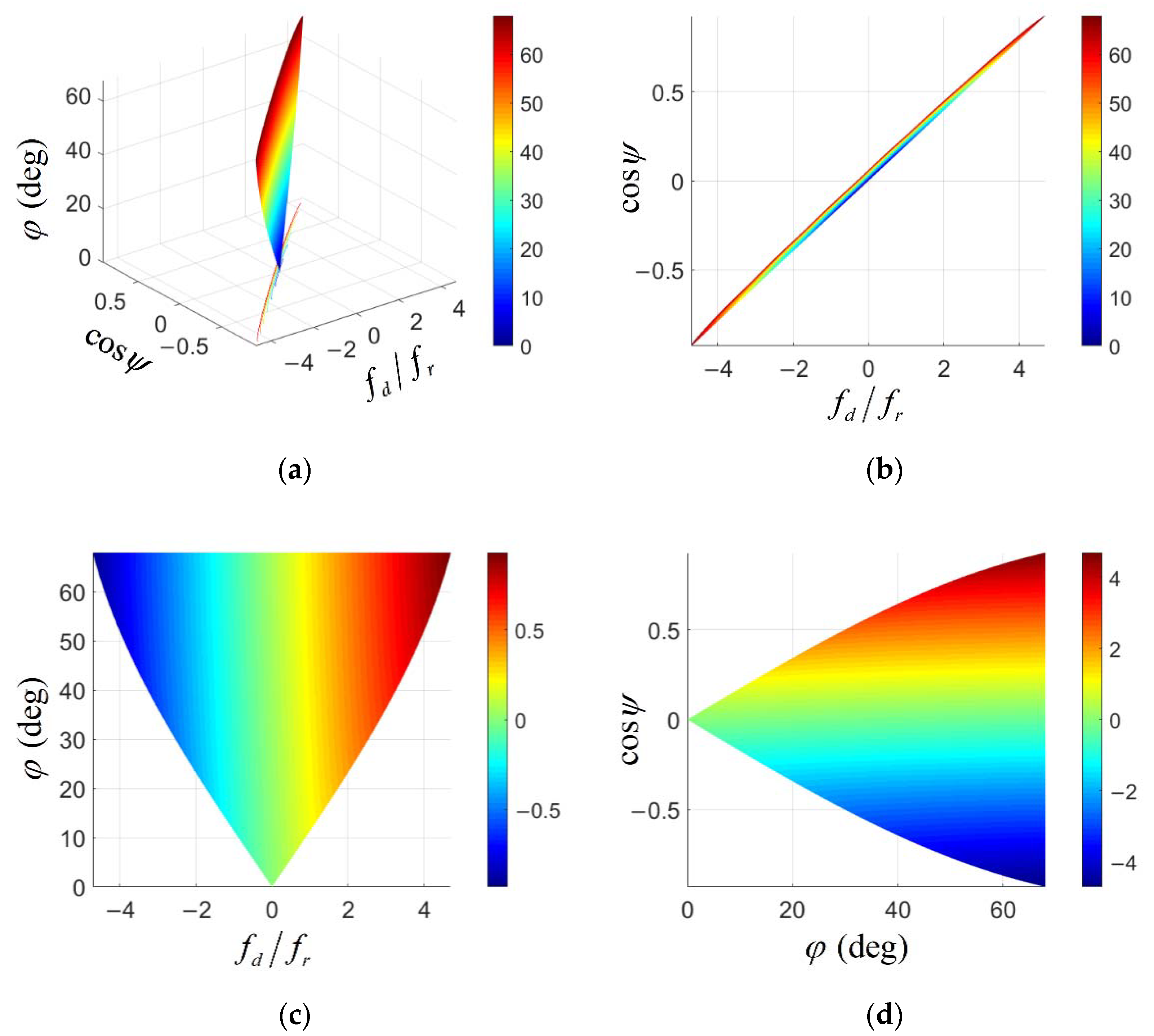
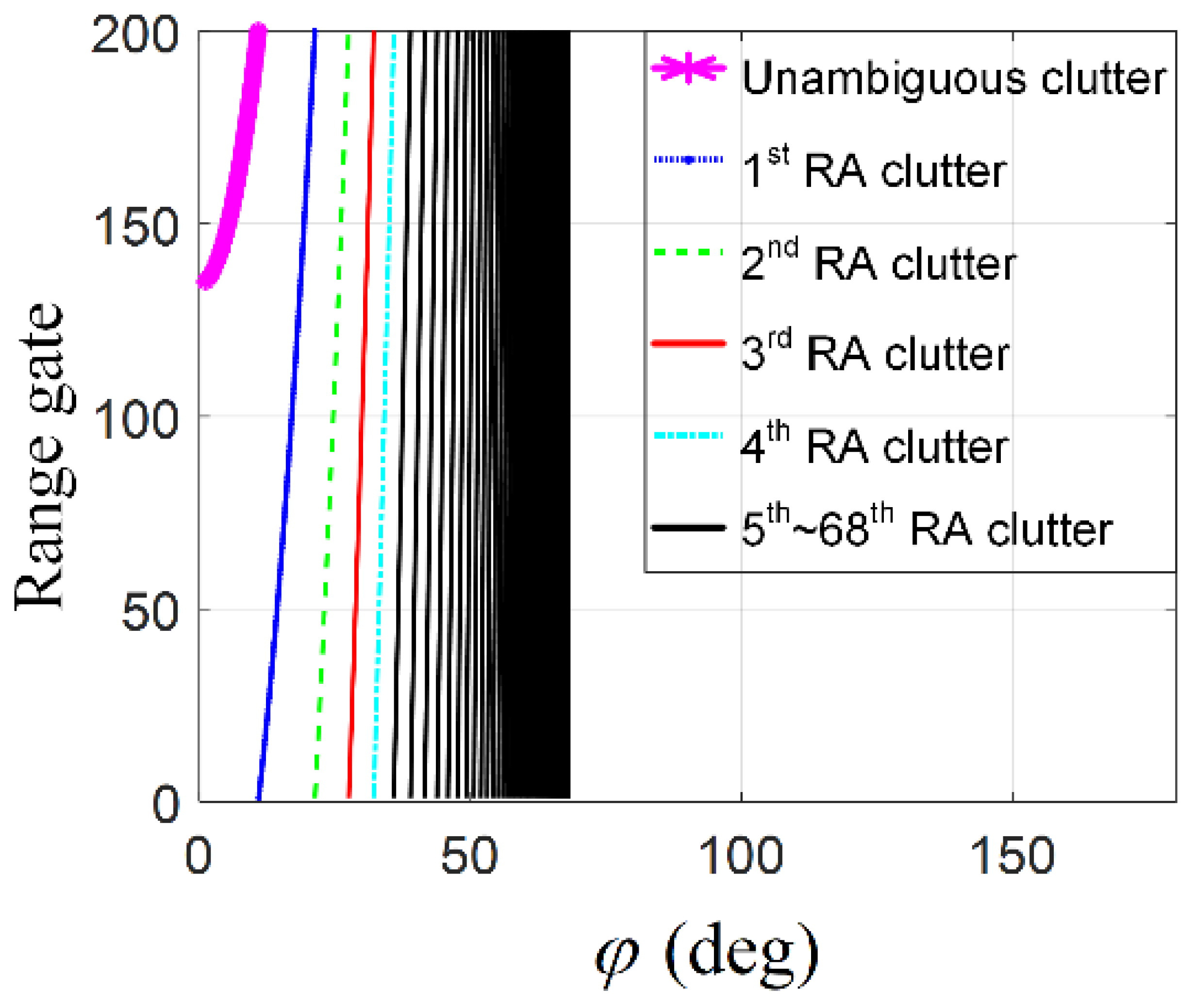
3.2.2. Doppler Distributions of Different RA Components in One Range Gate

The non-stationarity of the mainlobe clutter in the elevation dimension was discussed in the previous subsection, which focused on whether the clutter from different range gates had the same space–time distributions. In this subsection, the Doppler distribution of different RA components within one range gate. On the one hand, the mainlobe width in the Doppler dimension of a certain RA component with an elevation angle of ${\phi }_0$ can be calculated approximately as

$$\mathrm{\Delta }{B}_a\approx \frac{2V_p}{\lambda f_r}\sin {\phi }_0\left(\cos \left(\theta +\frac{\mathrm{\Delta }\theta }{2}\right)-\cos \left(\theta -\frac{\mathrm{\Delta }\theta }{2}\right)\right)$$

(24)

where $\mathrm{\Delta }\theta$ is the 3 dB mainlobe width of the azimuth angle. On the other hand, the difference in the Doppler dimension between two RA components in the same range gate with an elevation angle of ${\phi }_1$ and ${\phi }_2$ can be calculated as

$$\mathrm{\Delta }{f}_d=\frac{2V_p}{\lambda f_r}\cos \left(\theta +{\varphi }_c\right)\left(\sin {\phi }_1-\sin {\phi }_2\right)$$

(25)

As the velocity of SBEWR is 50 times more than that of AEWR, the values of these two indexes increase greatly. The theoretical mainlobe Doppler distributions of all RA components in the 138th range gate with the parameters presented in Table 1 are shown in Figure 4a,b for AEWR and SBEWR, respectively. The color in this figure is consistent with that of Figure 3b,d; $\mathrm{\Delta }{B}_a$ can be described by the length of an individual horizontal line, and $\mathrm{\Delta }{f}_d$ can be described by the difference of horizontal scale between two horizontal lines. Figure 4 illustrates that the $\mathrm{\Delta }{B}_a$ and $\mathrm{\Delta }{f}_d$ of the SBEWR are much larger than those of AEWR visually. The larger $\mathrm{\Delta }{B}_a$ and $\mathrm{\Delta }{f}_d$ are, the more auxiliary beams 3D-STAP methods need in the Doppler dimension.

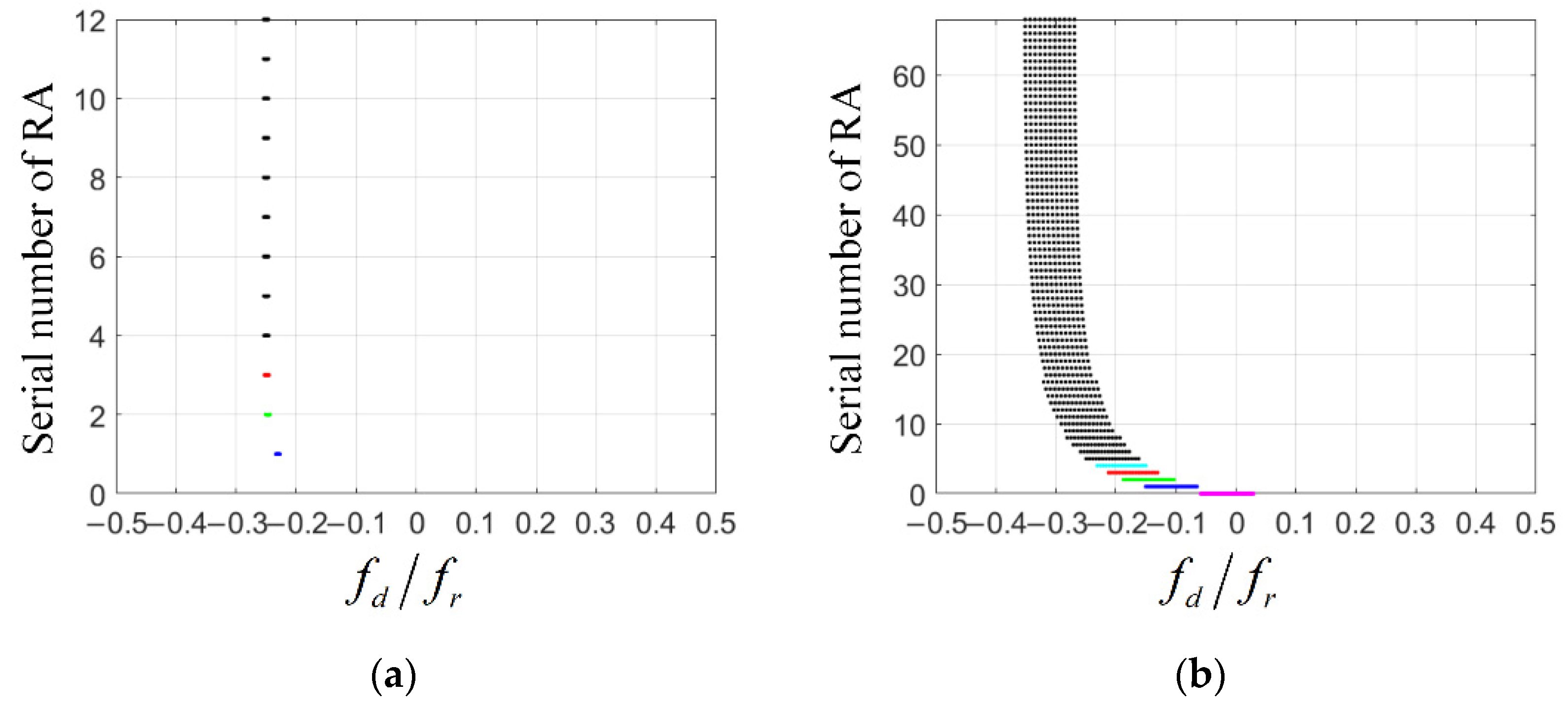
3.2.3. Clutter Degrees of Freedom (DOFs) in the Elevation Dimension

The number of RA can be calculated as

$$N_R=⌊\frac{2f_r{R}_{s\max }}{c}⌋$$

(26)

where $⌊\cdot ⌋$ denotes the rounding down operator, and $c$ and $R_{s\max }$ denote the speed of light and the maximum of the slant range, respectively. As the $R_{s\max }$ of the SBEWR is much larger than that of AEWR, the number of RAs for SBEWR is also much larger. According to Table 1, the numbers of RAs for SBEWR and AEWR are 12 and 68, respectively. The difference in the number of Ras will lead to the difference on the DOFs of the clutter in the elevation dimension, which can be calculated as [17]

$$DO{F}_{el}=\min \left\{M,N_R\right\}$$

(27)

As the number of array elements in the elevation dimension increases, the difference in the DOFs in the elevation dimension between SBEWR and AEWR will increase. The larger number of DOFs in the elevation dimension will increase the requirement for auxiliary beams in the elevation dimension for nonstationary clutter suppression.

4. Proposed Dimension-Reduced Structures for 3D-STAP Methods

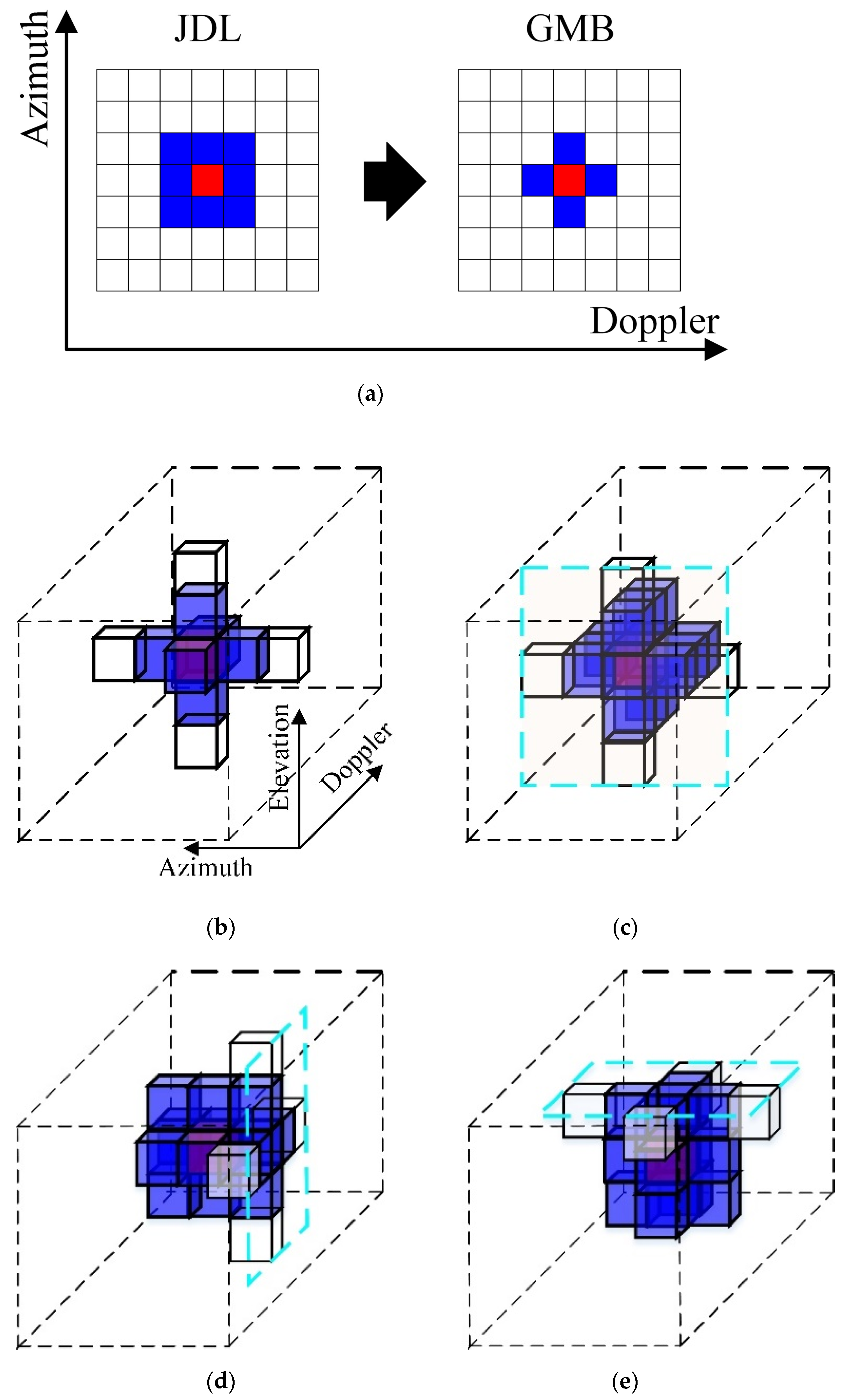
4.1. 3D-SDB

As mentioned in Section 2, the total number of required auxiliary beams for the 3D-JDL is $\left(2m+1\right)\left(2n+1\right)\left(2k+1\right)$. Because $m$, $n$ and $k$ are positive integers, the total number will not less than 27. When the demand for auxiliary beams in any dimension increases, which may be caused by severe RA or a larger mainlobe width in the Doppler dimension, the total number will correspondingly increase on the basis of 27. In order to reduce the total number, a feasible idea is to ensure the number of auxiliary beams in one or more dimensions is less than three. In terms of this goal, the idea of SDB, which is proposed in2D-STAP methods [20] and only has two spatial DOFs, is a good choice. By applying the idea of SDB to 3D-STAP methods, the dimension-reduced matrix in each dimension can be expressed, respectively, as

$$T_{\mathrm{SDB},\mathrm{el}}=\left[B_s\odot V_{se}\left(f_{se}\left(t\right)\right),B_d\odot V_{se}\left(f_{se}\left(t\right)\right)\right]\in {ℂ}^{M\times 2}$$

(28)

$$T_{\mathrm{SDB},\mathrm{az}}=\left[B_s\cdot V_{sa}\left(f_{sa}\left(t\right)\right),B_d\cdot V_{sa}\left(f_{sa}\left(t\right)\right)\right]\in {ℂ}^{N\times 2}$$

(29)

$$T_{\mathrm{SDB},\mathrm{d}}=\left[B_s\cdot V_d\left(f_d\left(t\right)\right),B_d\cdot V_d\left(f_d\left(t\right)\right)\right]\in {ℂ}^{K\times 2}$$

(30)

where $B_s$ and $B_d$ are the weight functions of sum beams and difference beams, respectively, such as the Chebyshev weight function and the Bayliss weight function. $\odot$ denotes the Hadamard product. Considering that the dimension-reduced matrix of SDB can be used in 1, 2 or 3 dimensions, there are seven different structures of 3D-SDB, which can be formulated, respectively, as follows:

$$T_{3\mathrm{DSDB},1}=T_{\mathrm{SDB},\mathrm{el}}\otimes T_{\mathrm{SDB},\mathrm{az}}\otimes T_{\mathrm{SDB},\mathrm{d}}$$

(31)

$$T_{3\mathrm{DSDB},2}=T_{\mathrm{JDL},\mathrm{el}}\otimes T_{\mathrm{SDB},\mathrm{az}}\otimes T_{\mathrm{SDB},\mathrm{d}}$$

(32)

$$T_{3\mathrm{DSDB},3}=T_{\mathrm{SDB},\mathrm{el}}\otimes T_{\mathrm{JDL},\mathrm{az}}\otimes T_{\mathrm{SDB},\mathrm{d}}$$

(33)

$$T_{3\mathrm{DSDB},4}=T_{\mathrm{SDB},\mathrm{el}}\otimes T_{\mathrm{SDB},\mathrm{az}}\otimes T_{\mathrm{JDL},\mathrm{d}}$$

(34)

$$T_{3\mathrm{DSDB},5}=T_{\mathrm{SDB},\mathrm{el}}\otimes T_{\mathrm{JDL},\mathrm{az}}\otimes T_{\mathrm{JDL},\mathrm{d}}$$

(35)

$$T_{3\mathrm{DSDB},6}=T_{\mathrm{JDL},\mathrm{el}}\otimes T_{\mathrm{SDB},\mathrm{az}}\otimes T_{\mathrm{JDL},\mathrm{d}}$$

(36)

$$T_{3\mathrm{DSDB},7}=T_{\mathrm{JDL},\mathrm{el}}\otimes T_{\mathrm{JDL},\mathrm{az}}\otimes T_{\mathrm{SDB},\mathrm{d}}$$

(37)

4.2. 3D-GMB

Apart from reducing the numbers of auxiliary beams in each dimension, another idea to reduce the total number of auxiliary beams is to change the relationships between the three dimensions from multiplication to summation. This idea is proposed by the 2D-GMB method [21] at first with a schematic diagram shown in Figure 5a. It illustrates that the value of both $n$ and $k$ are one for 2D-JDL and 2D-GMB, while the total number of the auxiliary beams for the 2D-JDL and 2D-GMB are $\left(2n+1\right)\left(2k+1\right)$ and $\left(2n+1\right)+\left(2k+1\right)-1$, respectively.

The 1D dimension-reduced matrixes are formulated as

$$T_{1\mathrm{DGMB},\mathrm{el}}=\left[V_{se}\left(f_{se}\left(t-m\right)\right),\cdots ,V_{se}\left(f_{se}\left(t-1\right)\right),V_{se}\left(f_{se}\left(t+1\right)\right),\cdots ,V_{se}\left(f_{se}\left(t+m\right)\right)\right]$$

(38)

$$T_{1\mathrm{DGMB},\mathrm{az}}=\left[V_{sa}\left(f_{sa}\left(t-n\right)\right),\cdots ,V_{sa}\left(f_{sa}\left(t-1\right)\right),V_{sa}\left(f_{sa}\left(t+1\right)\right),\cdots ,V_{sa}\left(f_{sa}\left(t+n\right)\right)\right]$$

(39)

$$T_{1\mathrm{DGMB},\mathrm{d}}=\left[V_d\left(f_d\left(t-k\right)\right),\cdots V_d\left(f_d\left(t-1\right)\right),V_d\left(f_d\left(t+1\right)\right),\cdots ,V_d\left(f_d\left(t+k\right)\right)\right]$$

(40)

When applying the idea of the GMB to the 3D-STAP methods, there are four different structures for the 3D-GMB, just as with the 3D-SDB. The schematic diagrams of the four structures are shown in Figure 5b–e, respectively. In the first case, the GMB is used in the elevation-azimuth-Doppler cube with the dimension-reduced matrix formulated as

$$T_{3\mathrm{DGMB},1}=\left[T_{3\mathrm{DGMB},\mathrm{el}}\left(t,t\right),T_{3\mathrm{DGMB},\mathrm{az}}\left(t,t\right),T_{3\mathrm{DGMB},\mathrm{d}}\left(t,t\right),V_{3\mathrm{D}}\left(t\right)\right]$$

(41)

where

$$T_{3\mathrm{DGMB},\mathrm{el}}\left(i,j\right)=T_{1\mathrm{DGMB},\mathrm{el}}\otimes V_{sa}\left(f_{sa}\left(i\right)\right)\otimes V_d\left(f_d\left(j\right)\right)\in {ℂ}^{MNK\times 2m}$$

(42)

$$T_{3\mathrm{DGMB},\mathrm{az}}\left(h,j\right)=V_{se}\left(f_{se}\left(h\right)\right)\otimes T_{1\mathrm{DGMB},\mathrm{az}}\otimes V_d\left(f_d\left(j\right)\right)\in {ℂ}^{MNK\times 2n}$$

(43)

$$T_{3\mathrm{DGMB},\mathrm{d}}\left(h,i\right)=V_{\mathrm{se}}\left(f_{\mathrm{se}}\left(h\right)\right)\otimes V_{\mathrm{sa}}\left(f_{\mathrm{sa}}\left(i\right)\right)\otimes T_{1\mathrm{DGMB},\mathrm{d}}\in {ℂ}^{MNK\times 2k}$$

(44)

In the second case, GMB is used in the elevation-azimuth plane with the dimension-reduced matrix formulated as

$${{\rm T}}_{3\mathrm{DGMB},2}=\left[T_{2\mathrm{DGMB},\mathrm{el},\mathrm{az}}\left(t-k\right),\cdots ,T_{2\mathrm{DGMB},\mathrm{el},\mathrm{az}}\left(t\right),\cdots T_{2\mathrm{DGMB},\mathrm{el},\mathrm{az}}\left(t+k\right)\right]$$

(45)

where

$$\begin{array}{ll}{T}_{2\mathrm{DGMB},\mathrm{el},\mathrm{az}}\left(j\right)= [& T_{1\mathrm{DGMB},\mathrm{el}}\otimes V_{sa}\left(f_{sa}\left(t\right)\right)\otimes V_d\left(f_d\left(j\right)\right)\\ & V_{se}\left(f_{se}\left(t\right)\right)\otimes T_{1\mathrm{DGMB},\mathrm{az}}\otimes V_d\left(f_d,\left(j\right)\right)\\ & \left.V_{se}\left(f_{se}\left(t\right)\right)\otimes V_{sa}\left(f_{sa}\left(t\right)\right)\otimes V_d\left(f_d\left(j\right)\right)\right]\in {ℂ}^{MNK\times \left(2m+2n+1\right)}\end{array}$$

(46)

Similarly, in the third and fourth cases, GMB are used in the elevation-Doppler plane and the azimuth-Doppler plane with the dimension-reduced matrixes formulated, respectively, as

$$T_{3\mathrm{DGMB},3}=\left[T_{2\mathrm{DGMB},\mathrm{el},\mathrm{d}}\left(t-n\right),\cdots ,T_{2\mathrm{DGMB},\mathrm{el},\mathrm{d}}\left(t\right),\cdots ,T_{2\mathrm{DGMB},\mathrm{el},\mathrm{d}}\left(t+n\right)\right]$$

(47)

$$T_{3\mathrm{DGMB},4}=\left[T_{2\mathrm{DGMB},\mathrm{az},\mathrm{d}}\left(t-m\right),\cdots ,T_{2\mathrm{DGMB},\mathrm{az},\mathrm{d}}\left(t\right),\cdots ,T_{2\mathrm{DGMB},\mathrm{az},\mathrm{d}}\left(t+m\right)\right]$$

(48)

where

$$\begin{array}{ll}{T}_{2\mathrm{DGMB},\mathrm{el},\mathrm{d}}\left(i\right)= [& T_{1\mathrm{DGMB},\mathrm{el}}\otimes V_{sa}\left(f_{sa}\left(i\right)\right)\otimes V_d\left(f_d\left(t\right)\right)\\ & V_{se}\left(f_{se}\left(t\right)\right)\otimes V_{sa}\left(f_{sa}\left(i\right)\right)\otimes T_{1\mathrm{DGMB},\mathrm{d}}\\ & \left.V_{se}\left(f_{se}\left(t\right)\right)\otimes V_{sa}\left(f_{sa}\left(i\right)\right)\otimes V_d\left(f_d\left(t\right)\right)\right]\in {ℂ}^{MNK\times \left(2m+2k+1\right)}\end{array}$$

(49)

$$\begin{array}{ll}{T}_{2\mathrm{DGMB},\mathrm{az},\mathrm{d}}\left(h\right)= [& V_{se}\left(f_{se}\left(h\right)\right)\otimes T_{1\mathrm{DGMB},\mathrm{az}}\otimes V_d\left(f_d\left(t\right)\right)\\ & V_{se}\left(f_{se}\left(h\right)\right)\otimes V_{sa}\left(f_{sa}\left(t\right)\right)\otimes T_{1\mathrm{DGMB},\mathrm{d}}\\ & \left.V_{se}\left(f_{se}\left(h\right)\right)\otimes V_{sa}\left(f_{sa}\left(t\right)\right)\otimes V_d\left(f_d\left(t\right)\right)\right]\in {ℂ}^{MNK\times \left(2n+2k+1\right)}\end{array}$$

(50)

4.3. 3D-SS-DDL

3D-SS-STAP [17] is a typical 3D-STAP method, which can dramatically reduce the spatial DOFs by subarray synthesis in element space while keeping the DOFs in time domain unchanged. It means that the total system DOF is $\left(M+N\right)K$ for 3D-SS. Note that 3D-SS is proposed for AEWR whose number of pulses is small. The value of $K$ is 16 for simulation in [17]. However, SBEWR needs a larger number of pulses for coherent integration due to a much larger detection range compared to AEWR. Therefore, if we directly apply 3D-SS for SBEWR, the system DOFs will be too large for real-time processing. As a typical element–space post-Doppler STAP method, DDL [22] can localize the clutter by transforming the signal into the Doppler domain and reduce the system DOFs significantly. The dimension-reduced matrix of DDL in Doppler can be expressed as

$$T_{\mathrm{DDL}}=\left[V_{\mathrm{d}}\left(f_{\mathrm{d}}\left(t-k\right)\right),\cdots ,V_{\mathrm{d}}\left(f_{\mathrm{d}}\left(t\right)\right),\cdots ,V_{\mathrm{d}}\left(f_{\mathrm{d}}\left(t+k\right)\right)\right]\in {ℂ}^{K\times \left(2k+1\right)}$$

(51)

where $k$ can decide the number of auxiliary beams whose value is $2k+1$ for DDL in the Doppler domain. Then the improved 3D dimension-reduced matrix can be formulated as

$$T_{3\mathrm{DSSDDL}}=T_{3\mathrm{DSS},\mathrm{S}}\otimes T_{\mathrm{DDL}}\in {ℂ}^{MNK\times \left(M+N\right)\left(2k+1\right)}$$

(52)

Obviously, the total number of auxiliary beams decreases to $\left(M+N\right)\left(2k+1\right)$ now.

5. Further Analysis and Discussion

5.1. Suitable Plans for 3D-SDB and 3D-GMB for SBEWR

In Section 4, seven and four different dimension-reduced structures were given for the 3D-SDB and 3D-GMB, respectively, which reduced the total number of auxiliary beams. It is difficult to distinguish the best structure, as the clutter suppression performance is dependent on not only the structure but also the distribution of the clutter. We can obtain good performance of clutter suppression only if the structure is matched with the distribution. Therefore, the key point here is to choose the most suitable plans for the 3D-SDB and 3D-GMB, respectively, from the structures based on the 3D distributions of non-stationary clutter which were analyzed in Section 3.

Firstly, as mentioned in Section 3.2.2, for the clutter of the GUT, the mainlobe width in Doppler $\mathrm{\Delta }{B}_a$ for SBEWR was much larger compared to the AEWR. In addition, the high velocity of SBWER amplified the effectiveness of the RA, so that different RA components were located in different Doppler bins, especially for the near-range components, which are shown in Figure 4. Therefore, to estimate the Doppler information of all the RA components in the GUT accurately by the training samples, more auxiliary beams are needed in the Doppler dimension. Then for the elevation dimension, the larger number of the RA components for SBEWR leads to the increase in the DOFs in this dimension. In addition, different RA components have different elevation angles. Hence, enough auxiliary beams are also needed in the elevation dimension. Finally, as shown in Figure 2c, the clutter distributes homogeneous in the elevation-Doppler plane. In a certain Doppler bin, different elevation angles correspond to a similar value of $\cos \psi$, which means that different elevation components are mostly located in the same azimuth bin. Therefore, only a few auxiliary beams are needed in the azimuth dimension to achieve effective CCM estimation. In summary, more auxiliary beams are needed in both Doppler and elevation dimensions, while the demand for auxiliary beams is much lower for the azimuth dimension. Therefore, the 3D-SDB6, which performs the SDB in the azimuth dimension and is expressed by Equation (36), is the most suitable plan for 3D-SDB on non-stationary clutter suppression for SBEWR according to the analysis above. In addition, the distribution of clutter in the elevation-azimuth plane is also homogeneous, as illustrated by Figure 2d. Considering that the demand for auxiliary beams in the Doppler dimension is larger than the demand in the azimuth dimension, performing GMB in the elevation-azimuth plane is more suitable than in the elevation-Doppler plane. Further, because of the non-homogeneous distribution in the azimuth-Doppler plane, performing GMB in the azimuth-Doppler plane is not a suitable plan. That is to say, the 3D-GMB2, which is expressed by Equation (45), is the most suitable plan for the 3D-GMB.

5.2. Computational Complexity Analysis

The floating operations (FLOPS) of the 3D-STAP methods are calculated to analyze the computational complexity in this subsection. Note that both a complex multiplication and a complex summation are counted as one basic FLOP here for a reasonable approximation [23]. The general values of the FLOPS for the 3D-STAP methods are presented in

Table 2. General values of FLOPS for 3D-STAP methods.

Operations	FLOPS
Filter and CCM estimation	$\left(2L+1\right)N_D^2{N}_B^2+\left(4MNK-2\right)\left(L+1\right)N_D{N}_B$
Inverse of CCM	$L{N}_D\left(N_B^3+N_B^2+N_B\right)$
Calculation of optimal weight	$4N_B^2+2MNK{N}_B-MNK-1$
Adaptive filter	$\left(2MNK-1\right)L{N}_D$

, where $N_D$ denotes the number of divided Doppler filters, and $N_B$ denotes the total number of auxiliary beams. According to Table 2, the curve that indicates the relationship between the FLOPS and $N_B$ is shown in Figure 6 with $N_D=128$ and other main parameters listed in Table 1. This illustrates that the relationship is not linear. As $N_B$ grows larger, the increase in the FLOPS becomes faster. The relationship further indicates the necessity to reduce the total number of auxiliary beams due to the computational complexity.

5.3. A Limitation of the 3D-STAP Methods

The relationship between the elevation angle and the slant range for SBEWR can be expressed as

$$\phi =\arcsin \left(R_e/R_s\cdot \sin \left(R/R_e\right)\right)$$

(53)

The relationship is described by the range–elevation angle curves shown in Figure 7 for all 200 range gates. An individual range–elevation angle curve describes the distribution of the elevation angle for an individual RA component from all range gates. The curvatures of the curves indicate the range-variant property of the distributions. Figure 7 illustrates that the curvatures of the near-range RA components with smaller elevation angles are much larger than the curvatures of the far-range RA components with larger elevation angles, which indicates that the distributions of elevation angles for the near-range RA components have a higher level of range variance. Therefore, when using the data of the other range gates to estimate the CCM of GUT, the positions of the 3D notches for near-range RA components will be biased and shallow, which will lead to a performance loss compared to the far-range RA components.

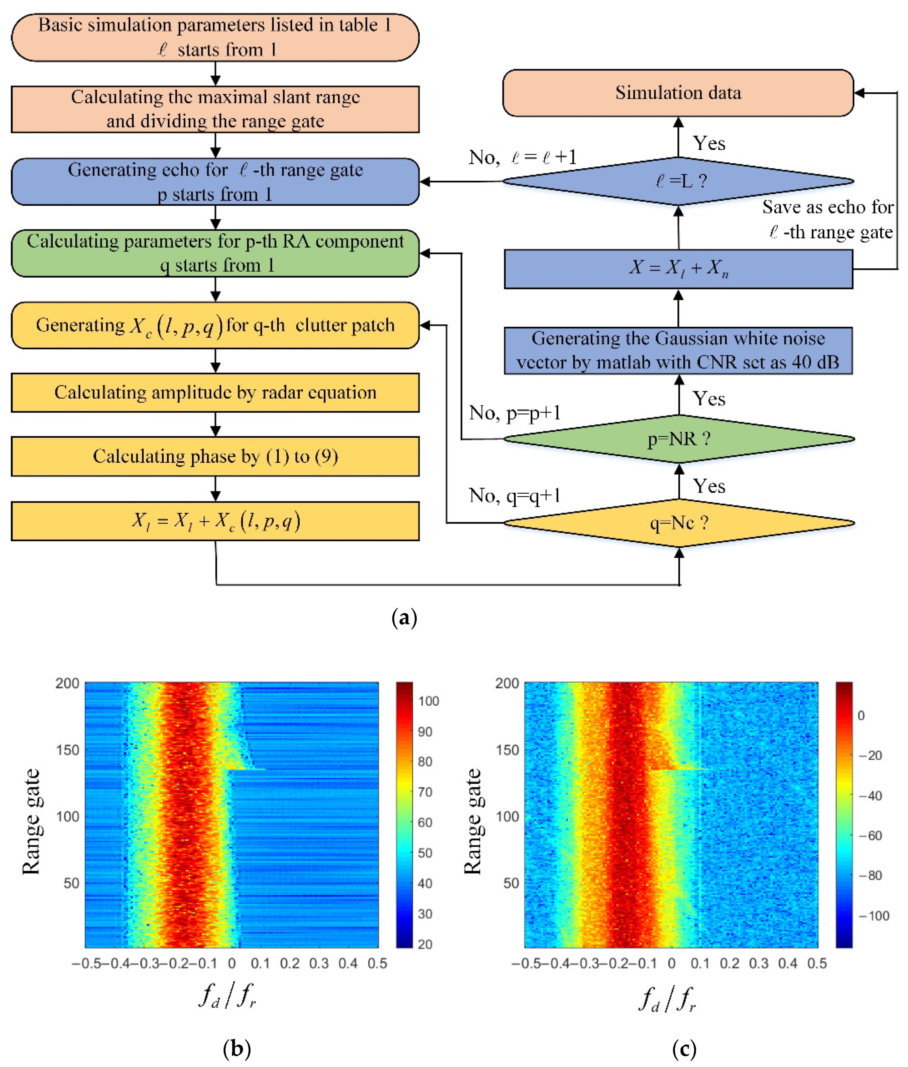
6. Simulation Experiments

6.1. Data Description

The echo of clutter for SBEWR was simulated with the main parameters listed in Table 1 according to the classic Ward model [6,7,24]. The detailed steps of echo simulation are shown in Figure 8a. The 256 elements were synthesized to eight subarrays in the azimuth dimension. In addition, the value of $N_c$ was 1800. Note that the value of $k$ and $f_r$ are 128 and 5000, respectively. In this case, the time of a CPI for the simulated data is 0.0256 s. Considering this short time and the stable velocity which is calculating by Newton’s laws of motion and the law of universal gravitation, the velocity of the platform is reasonably assumed as a constant here. The range-Doppler spectrum of the simulated data after common beam forming (CBF) in elevation is shown in Figure 8b. It illustrates that the general spectral lines were curved rather than straight, especially for the curved spectral lines of the near range RA components in the 135th–200th range gate. The range-Doppler spectrum is consistent with the theoretical one shown in Figure 3d and showed the non-stationarity of the clutter for SBEWR. Then the clutter suppression result of the JDL [25] which is one of typical the 2D-STAP methods is shown in Figure 8c, which illustrates that neither the mainlobe width nor the curved spectral lines can be suppressed effectively by the conventional 2D-STAP methods.

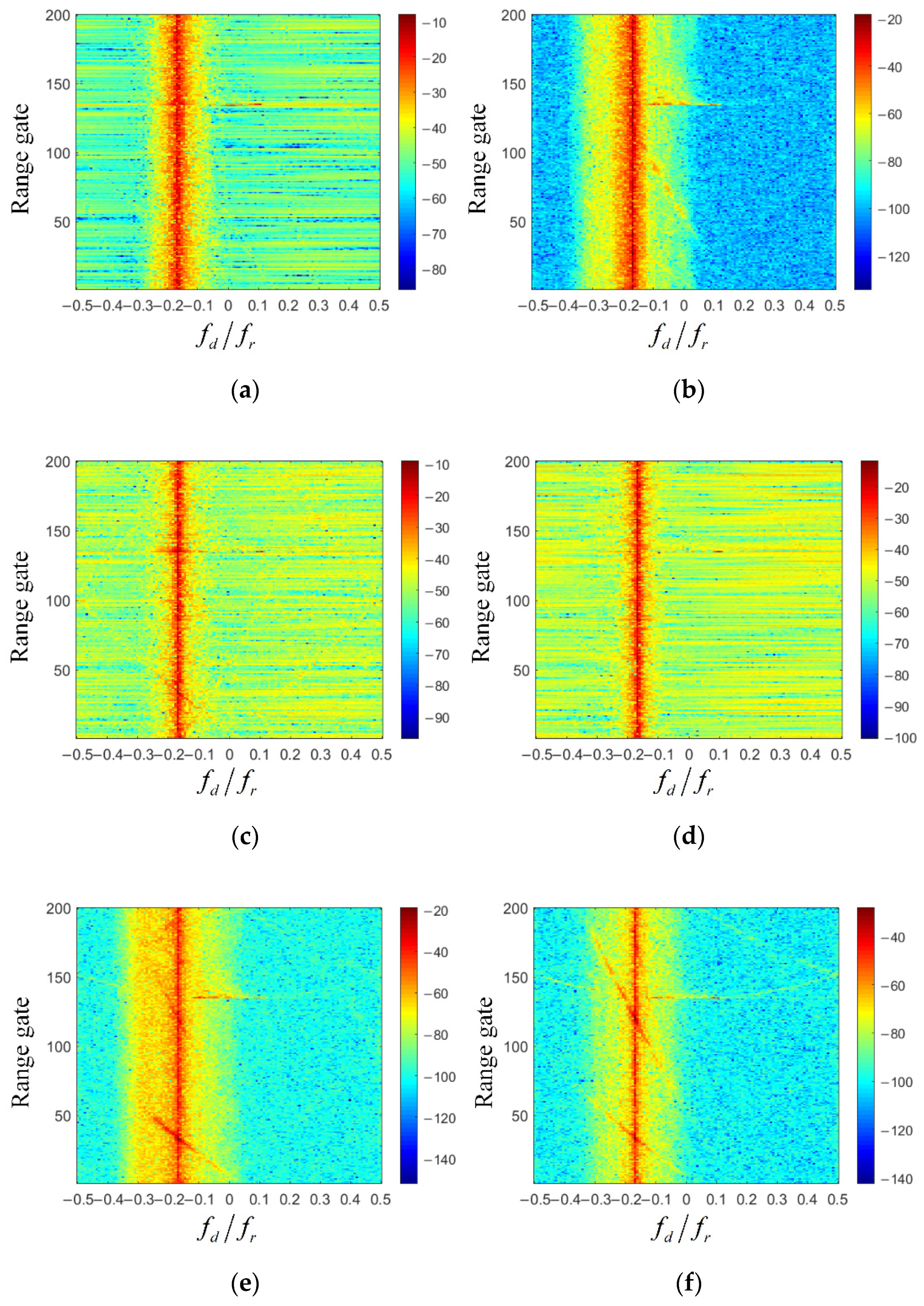
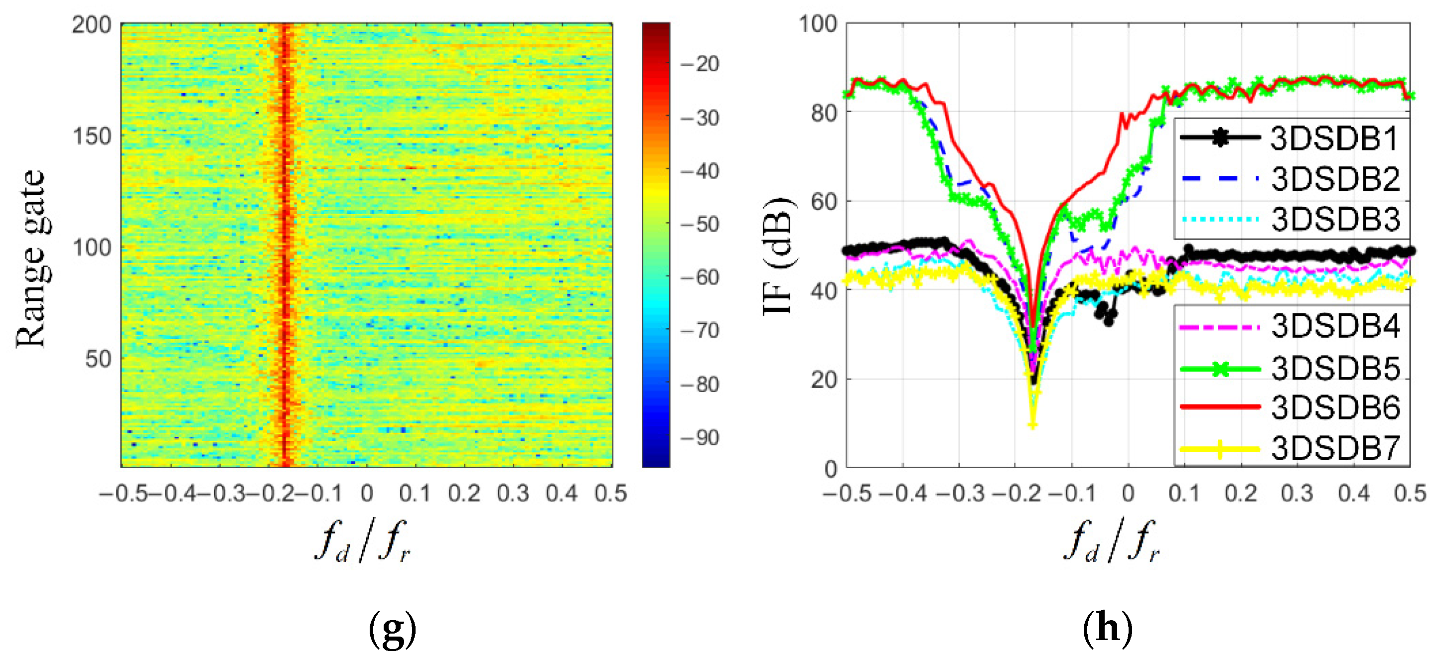
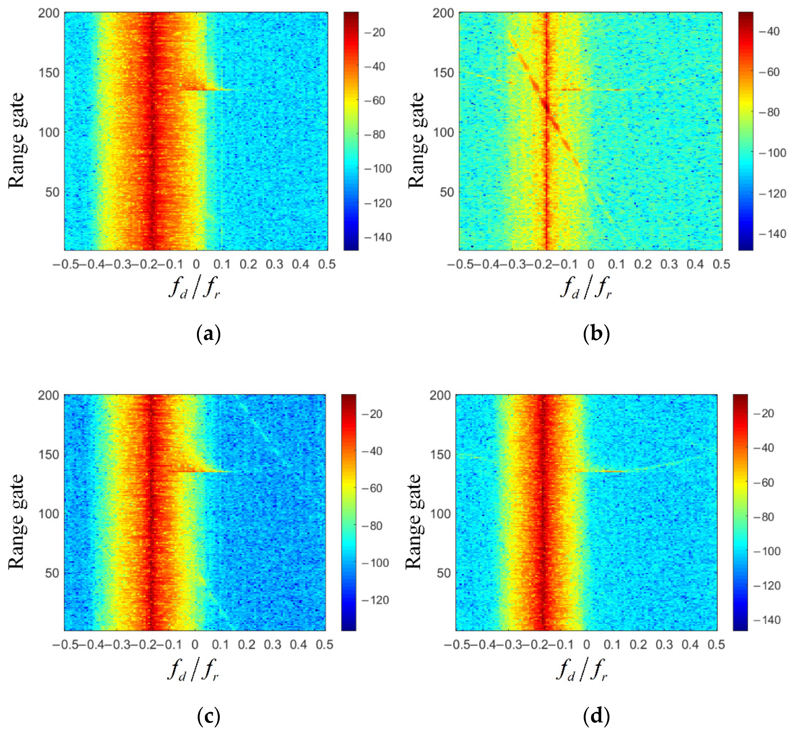
6.2. Experiment 1: Performance Analysis of Seven Structures for 3D-SDB

In this experiment, the performances of the seven structures described in Section 4.1 for 3D-SDB on non-stationary clutter suppression were analyzed. The non-stationary clutter suppression results of seven structures are shown in Figure 9a–f, while the improvement factor (IF) curves of the 138th range gate are shown in Figure 9g. Itis worth mentioning that the response pattern of STAP will distort when the radial velocity of the moving target is close to zero. In this case, the suppression performance of mainlobe clutter and IF which is used to evaluate the performance of clutter suppression will decrease rapidly. Therefore, there is a notch in the IF curve. Figure 9 illustrates that 3D-SDB6 has the widest mainlobe width and highest IF compared to the other six structures, which verifies that 3D-SDB6 is the most suitable plan for the 3D-SDB on the non-stationary clutter suppression for SBEWR. When using SDB in the Doppler or elevation dimension, the system DOFs in these two dimensions may not satisfy the demands for auxiliary beams in the corresponding dimensions. Therefore, the performances of the other structures were worse. In addition, comparing Figure 9e,g, one can find that the performance of 3D-SDB5 was much better than that of 3D-SDB7. This result indicates that the SDB was more unsuitable in the Doppler dimension compared to the elevation dimension. In other words, the demand for auxiliary beams in the Doppler dimension was much larger than that in the elevation dimension.

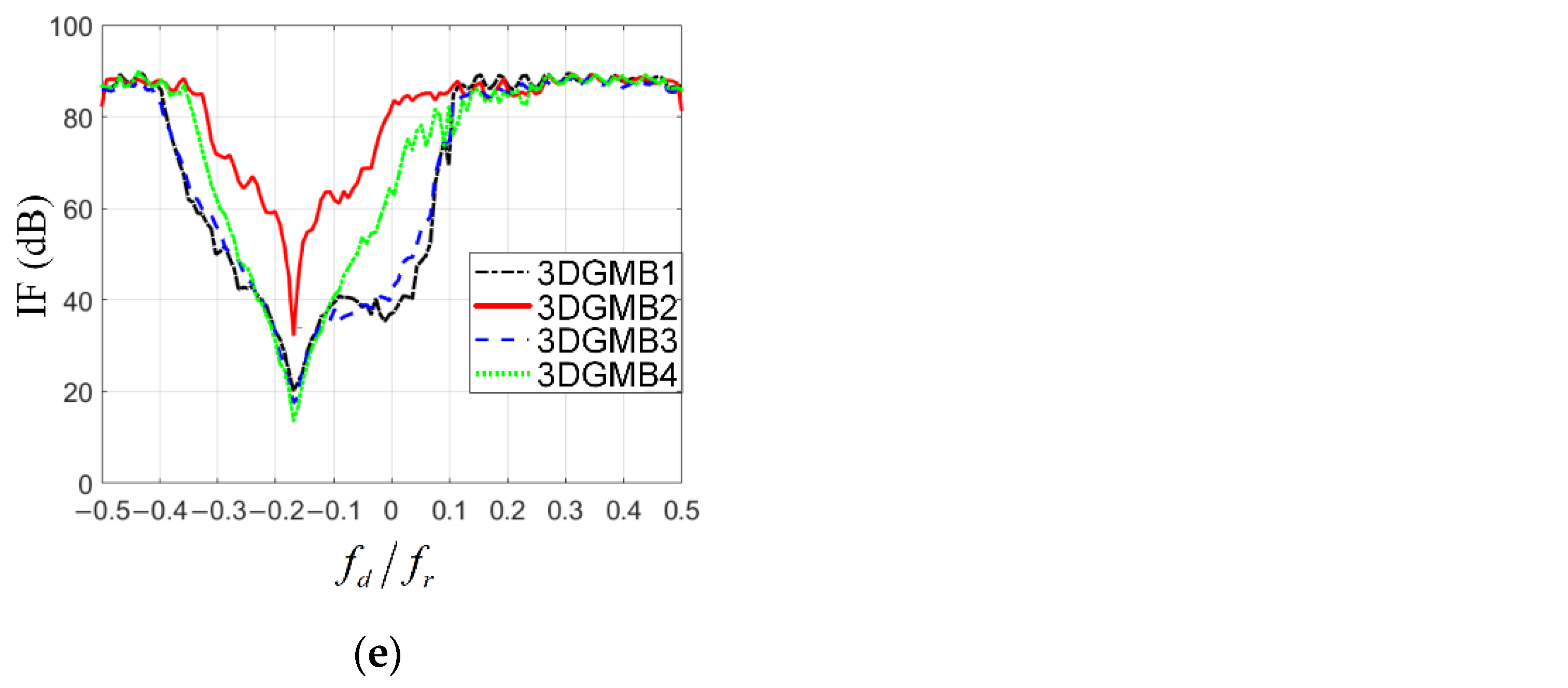
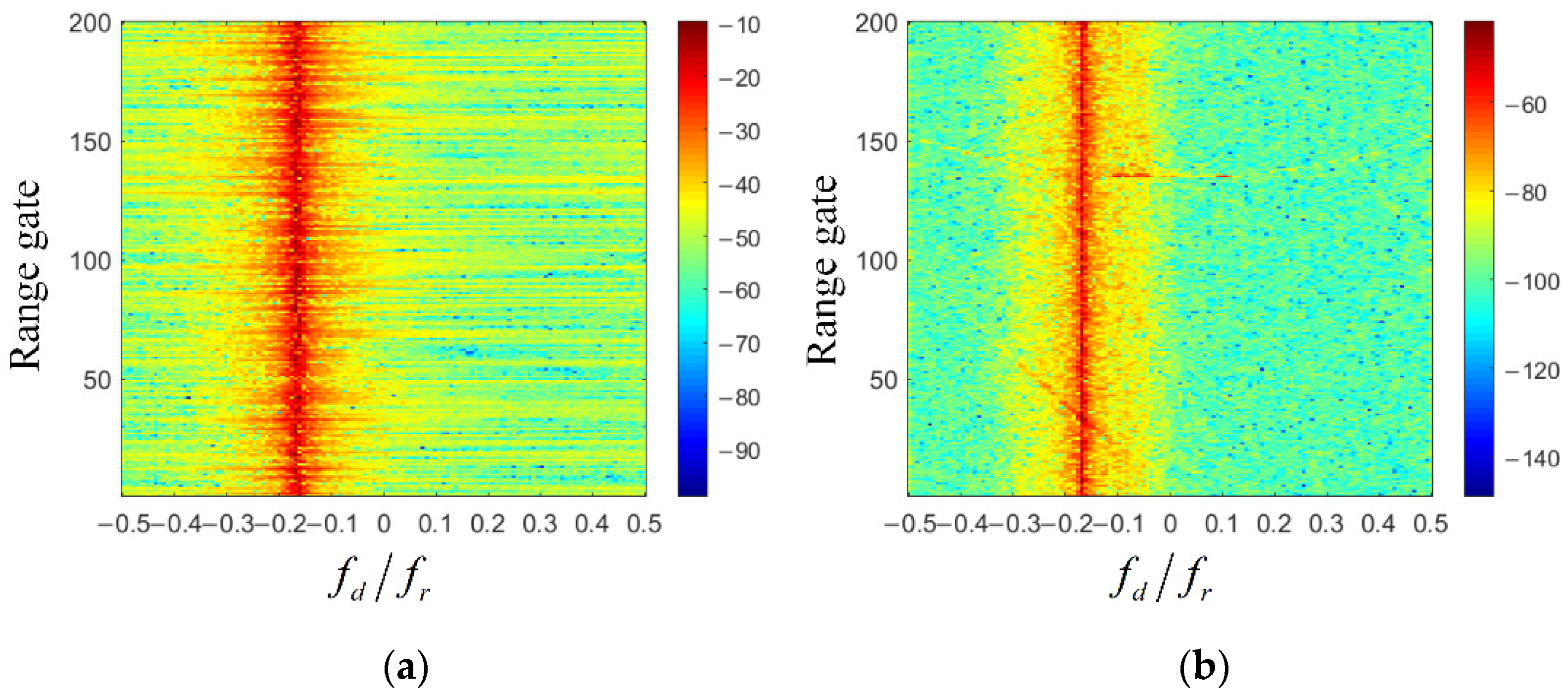
6.3. Experiment 2: Performance Analysis of the Four Structures for 3D-GMB

In this subsection, the performances of the four structures are analyzed for the 3D-GMB proposed in Section 4.2. The non-stationary clutter suppression results are given in Figure 10a–d. The IF curves of the 138th range gate are shown in Figure 10e. In terms of the mainlobe width and IF, Figure 10 illustrates that the performances of 3D-GMB1, 3D-GMB3, 3D-GMB4 and 3D-GMB2 are becoming better and better in succession. According to the result, we can find the same regularity as Section 6.2, where the demands for auxiliary beams in the Doppler, elevation and azimuth dimensions became larger in succession. The 3D-GMB2 also proved to be the most suitable plan of the 3D-GMB on the nonstationary clutter suppression for SBEWR.

6.4. Experiment 3: Performance Analysis for 3D-SS-DDL

In this subsection, the performances are analyzed for the 3D-SS-DDL detailed in Section 4.3. Three cases where the numbers of auxiliary beams in the Doppler dimension were one, three and five, respectively, are discussed here. The non-stationary clutter suppression results are given in Figure 11a–c. In addition, the IF curves of the 138th range gate are shown in Figure 11d. Figure 11 illustrates that the clutter suppression performance was poor when there was only one auxiliary beam in the Doppler dimension. Meanwhile, when the number of auxiliary beams increased from three to five, the performance seemed not to change greatly. The result may be caused by the restriction of the RMB rule. When the number of auxiliary beams in the Doppler is five, the number of independent and identically distributed samples should not have been less than 240 for accurate estimation of CCM. However, there are only 200 range gates in the simulated data, so the RMB rule could not be satisfied.

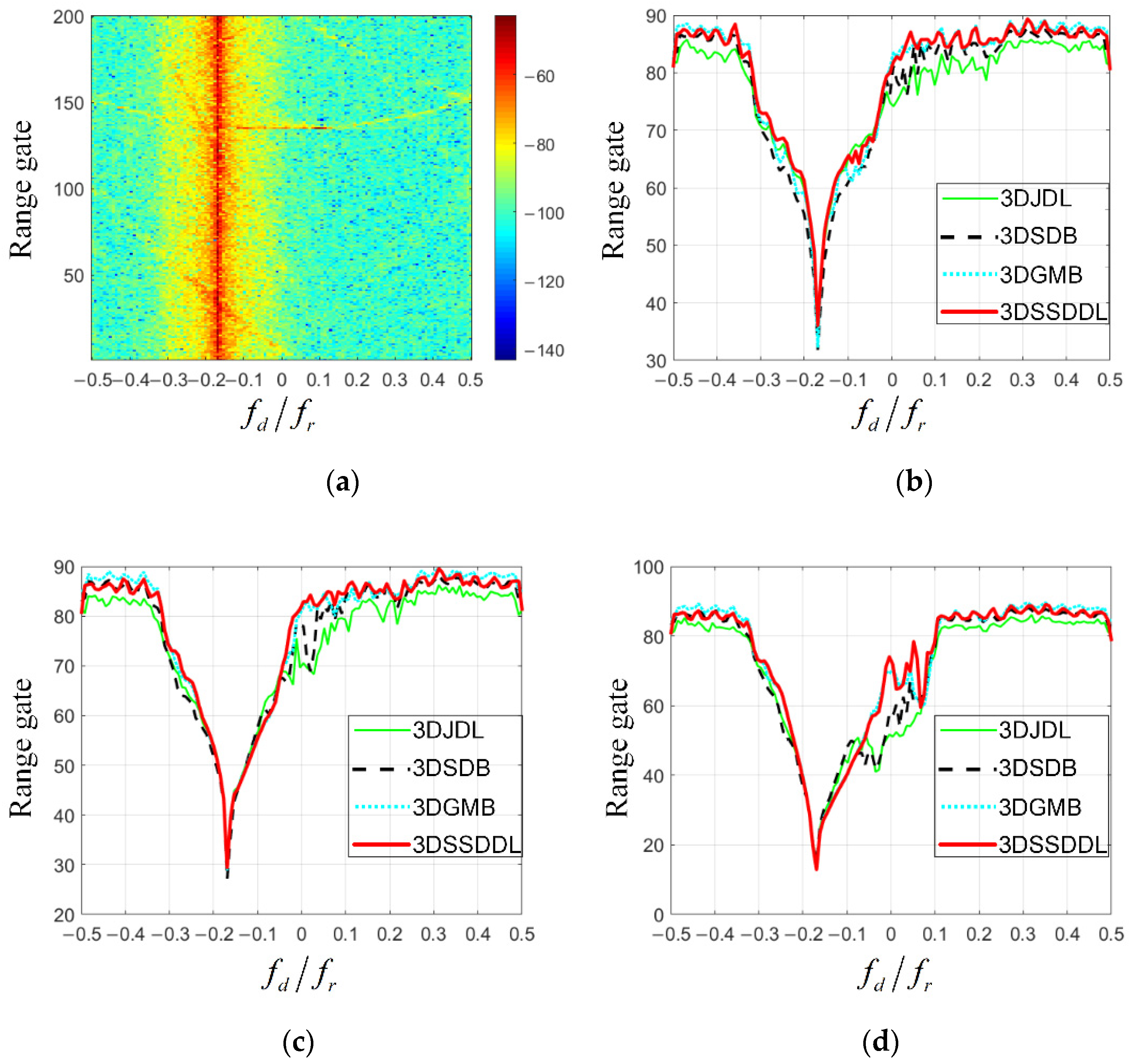
6.5. Experiment 4: Performance Comparison among the 3D-JDL and Three Proposed Methods

The performances of the 3D-JDL and the three improved 3D-STAP methods proposed in Section 4 are compared in this subsection. According to the results in the last three subsections, we select 3D-SDB6 (5 × 2 × 5), 3D-GMB2 ((9 + 3) × 3) and 3D-SS-DDL ((16 + 8) × 3) as the representations of the 3D-SDB, 3D-GMB and 3D-SS-DDL, respectively. The clutter suppression result of the 3D-JDL (5 × 5 × 5) is shown in Figure 12a. The IF curves of the 138th range gate for the four methods are shown in Figure 12b. This illustrates that the performances of the four methods are close. The IF curves of three proposed methods were a bit higher than those of 3D-JDL in the region of the sidelobe. Generally, the 3D-SS-DDL had the best performance.

It is worth mentioning that there were residual slope and curved spectral lines in the range-Doppler spectrums shown by Figure 9, Figure 10, Figure 11 and Figure 12. The spectral lines belonged to the near-range clutter components which locate inside or near the mainlobe. The components were not well suppressed because of the high level of range-variant property, mentioned in Section 5.3 and as a general limitation of the 3D-STAP methods.

In addition, in order to take the potential unanticipated issues into account so that our simulation can be as real as possible. The experiments in the presence of array error, which might occur in the field data, were conducted. The results with 3% array error in the azimuth dimension are shown in Figure 12c. It illustrates that the four methods are not sensitive to the array error in the azimuth. The impact on the IF curves is slight. Furthermore, the results with 3% array error both in the azimuth and elevation dimension are given in Figure 12d. It illustrates that the IF curves decrease rapidly in the region from about −0.05 to 0.1, where the near-range RA components are mainly located. The phenomenon can be explained by the limitation of 3D-STAP methods which is analyzed in Section 5.3 as well. Obviously, the array error in the elevation dimension enlarged the limitation. Figure 12c,d also shows that 3D-SS-DDL and 3D-GMB are more robust compared to the other two methods in terms of the array error.

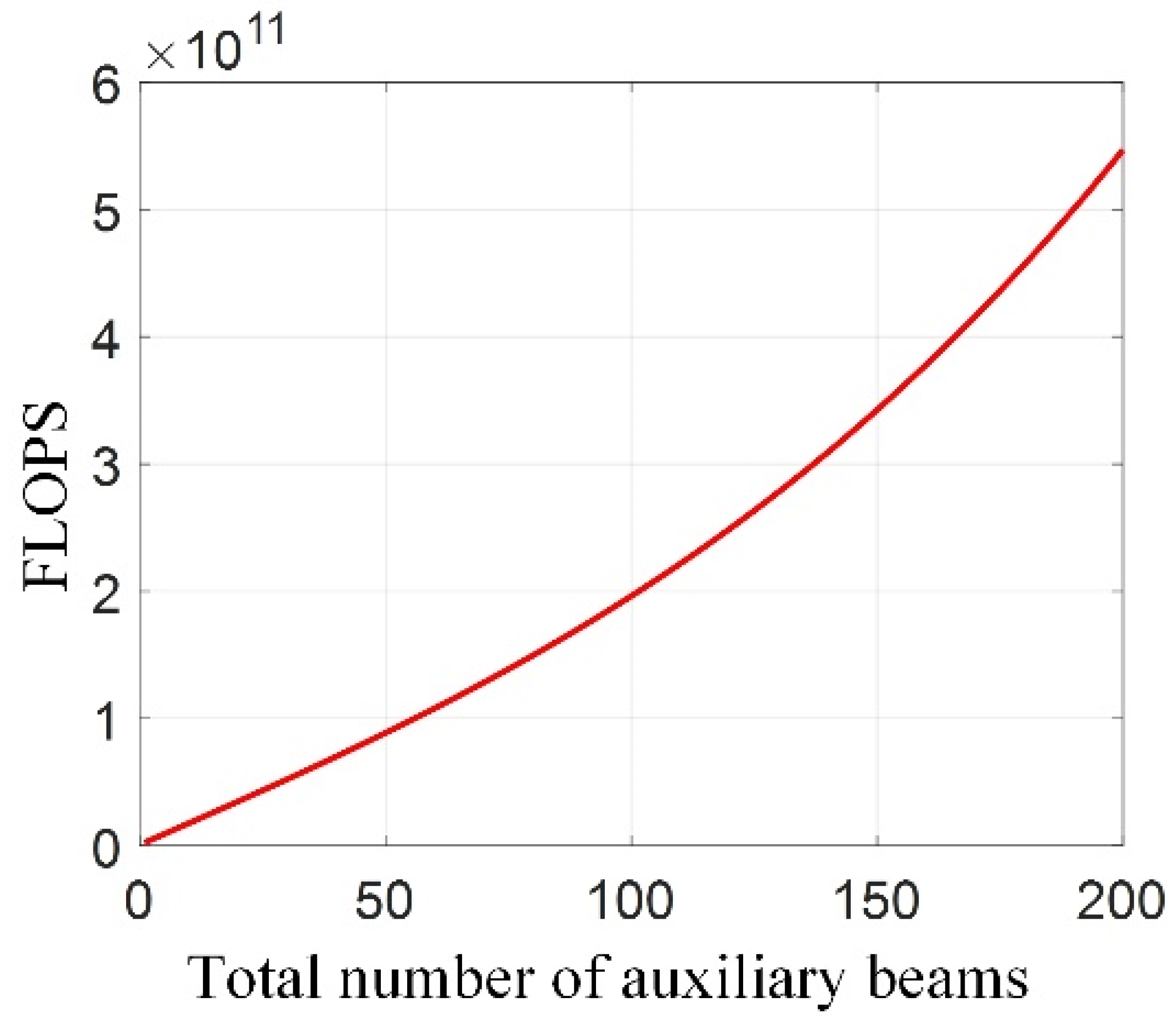
6.6. Experiment 5: Computational Complexity Comparison

After comparing the performance of the typical 3D-STAP methods and the proposed three 3D-STAP methods, the computational complexities of five methods are compared in this subsection. In terms of the total number of auxiliary beams, the ascending order is 3D-GMB (36) < 3D-SDB (50) < 3D-SS-DDL (72) < 3D-JDL (125) < 3D-SS (3072). Furthermore, in order to compare the computational complexities in a more quantitative way, the FLOPS of the five methods were calculated according to Table 2. The concrete calculation results are presented in

Table 3. Concrete values of FLOPS for the five 3D-STAP methods.

Methods	FLOPS
3D-JDL (5 × 5 × 5)	$2.633\times {10}^{11}$
3D-SDB (5 × 2 × 5)	$8.874\times {10}^{10}$
3D-GMB ((9 + 3) × 3)	$6.298\times {10}^{10}$
3D-SS ((16 + 8) × 128)	$5.892\times {10}^{12}$
3D-SS-DDL ((16 + 8) × 3)	$1.325\times {10}^{11}$

while four significant digits are kept. Obviously, the proposed three methods reduced the computational complexities effectively compared to the typical methods, especially for 3D-SS-DDL which uses DDL to reduce the system of DOFs in the Doppler domain significantly compared to 3D-SS.

7. Conclusions

In this article, focusing on the non-stationary clutter suppression in SBEWR, three improved dimension-reduced structures of 3D-STAP methods were proposed and analyzed. First, the signal model and 3D distributions of the non-stationary clutter are analyzed for SBEWR, which indicated why the 3D-STAP methods have better performance on the nonstationary clutter suppression compared to conventional 2D-STAP methods. Then, three differences in non-stationary clutter between SBEWR and AEWR caused by their differences in slant range, platform velocity and beam steering in elevation were discussed, respectively. The discussion became the theoretical basis for choosing the number of auxiliary beams in each dimension. Then, three improved dimension-reduced structures of 3D-STAP methods were proposed in detail based on two typical 3D-STAP methods, 3D-JDL and 3D-SS. The proposed three methods reduced the required total number of auxiliary beams. Thereby, the demands on the training samples and computational complexities were reduced. Finally, simulation experiments were conducted to verify the correctness and effectiveness of the proposed 3D-STAP methods. The simulation results show that the proposed 3D-STAP methods had better performance on the nonstationary clutter suppression in SBEWR with fewer computational complexities.

By combining the discussion in Section 5.1 and the simulation results, the suggestions for choosing the number of auxiliary beams in each dimension are summarized as follows. The Doppler dimension needs the largest number of auxiliary beams because of the severe widening of the mainlobe width in this dimension. The elevation dimension also needs a certain number of auxiliary beams due to the high number of RA components and their different values of elevation angle. The azimuth dimension needs the fewest auxiliary beams due to the homogeneous distributions of the non-stationary clutter in the elevation-Doppler plane.

Though the performance of the proposed methods is better on the nonstationary clutter suppression in SBEWR, the proposed methods also have limitations. Note that the distribution of the elevation angle for an individual RA component has a range-variant property; the property will degrade the accuracy of CCM estimation and make the positions of the 3D notches biased and shallow. Considering that the near-range RA components have a much higher level of range variance, there will be a performance loss for the near-range RA components compared to the far-range RA components when using the proposed 3D-STAP methods to suppress the nonstationary clutter in SBEWR.

Considering that SBEWR is at the pre-research stage now and there is not any SBEWR system in use in the world [26], the proposed methods were verified by the simulated data just like the most current papers on SBEWR [19,27,28,29,30,31,32]. More research will be promoted once we obtain a real dataset in the future.

References

1. Li, H.; Liao, G.; Xu, J.; Lan, L. An Efficient Maritime Target Joint Detection and Imaging Method with Airborne ISAR System. Remote Sens. 2022, 14, 193. [Google Scholar] [CrossRef]
2. Li, Y.; Huo, T.; Yang, C.; Wang, T.; Wang, J.; Li, B. An Efficient Ground Moving Target Imaging Method for Airborne Circular Stripmap SAR. Remote Sens. 2022, 14, 210. [Google Scholar] [CrossRef]
3. Han, J.; Cao, Y.; Wu, W.; Wang, Y.; Yeo, T.-S.; Liu, S.; Wang, F. Robust GMTI Scheme for Highly Squinted Hypersonic Vehicle-Borne Multichannel SAR in Dive Mode. Remote Sens. 2021, 13, 4431. [Google Scholar] [CrossRef]
4. Li, K.; Mangiat, S.; Zulch, P.; Pillai, U. Clutter Impacts on Space Based Radar GMTI: A Global Perspective. In Proceedings of the IEEE Aerospace Conference, Big Sky, MT, USA, 18 June 2007; pp. 1–15. [Google Scholar]
5. Brennan, L.; Reed, L. Theory of Adaptive Radar. IEEE Trans. Aerosp. Elect. Syst. 1973, 9, 237–252. [Google Scholar] [CrossRef]
6. Klemm, R. Principles of Space-Time Adaptive Processing, 3rd ed.; IET: London, UK, 2006; pp. 159–177. [Google Scholar]
7. Guerci, J. Space-Time Adaptive Processing for Radar, 2nd ed.; Artech House: London, UK, 2014; pp. 115–170. [Google Scholar]
8. Melvin, W. A stap over view. IEEE Trans. Aerosp. Elect. Syst. 2004, 19, 19–35. [Google Scholar] [CrossRef]
9. Borsari, G. Mitigating effects on stap processing caused by an inclined array. In Proceedings of the 1998 IEEE Radar Conference, Dallas, TX, USA, 11–14 May 1998; pp. 135–140. [Google Scholar]
10. Himed, B.; Zhang, Y.; Hajjari, A. Stap with angle-Doppler compensation for bistatic airborne radars. In Proceedings of the 2002 IEEE Radar Conference, Long Beach, CA, USA, 25 April 2002; pp. 311–317. [Google Scholar]
11. Jia, F.; He, Z.; Li, J.; Qian, J. Adaptive angle-Doppler compensation in airborne phased radar for planar array. In Proceedings of the 13th International Conference on Signal Processing (ICSP), Chengdu, China, 6–10 November 2016; pp. 1585–1588. [Google Scholar]
12. Lapierre, F.; Verly, J.; Van Droogenbroeck, M. New solutions to the problem of range dependence in bistatic STAP radars. In Proceedings of the 2003 IEEE Radar Conference, Huntsville, AL, USA, 8 May 2003; pp. 452–459. [Google Scholar]
13. Wu, J.; Wang, T.; Meng, X.; Bao, Z. Clutter suppression for airborne nonsidelooking radar using ERCB-STAP algorithm. IET Radar Sonar Navig. 2010, 4, 497–506. [Google Scholar] [CrossRef]
14. Shen, M.; Meng, X.; Zhang, L. Efficient adaptive approach for airborne radar short-range clutter suppression. IET Radar Sonar Navig. 2012, 6, 900–904. [Google Scholar] [CrossRef]
15. Wang, Z.; Xie, W.; Duan, K.; Gao, F.; Wang, Y. Short-range clutter suppression based on subspace projection preprocessing for airborne radar. In Proceedings of the 2016 CIE International Conference on Radar, Guangzhou, China, 10–13 October 2016; pp. 1–4. [Google Scholar]
16. Hale, T.; Temple, M.; Raquet, J.; Oxley, M.; Wicks, M. Localized three-dimensional adaptive spatial-temporal processing for airborne radar. In Proceedings of the RADAR 2002, Edinburgh, UK, 15–17 October 2002; pp. 191–195. [Google Scholar]
17. Duan, K.; Xu, H.; Yuan, H.; Xie, H.; Wang, Y. Reduced-DOF Three-Dimensional STAP via Subarray Synthesis for Nonsidelooking Planar Array Airborne Radar. IEEE Trans. Aerosp. Elect. Syst. 2020, 56, 3311–3325. [Google Scholar] [CrossRef]
18. Reed, I.; Mallett, J.; Brennan, L. Rapid Convergence Rate in Adaptive Arrays. IEEE Trans. Aerosp. Elect. Syst. 1974, 10, 853–863. [Google Scholar] [CrossRef]
19. Pillai, S.; Himed, B.; Li, K. Effect of earth’s rotation and range foldover on space-based radar performance. IEEE Trans. Aerosp. Elect. Syst. 2006, 42, 917–932. [Google Scholar] [CrossRef]
20. Brown, R.; Schneible, R.; Wicks, M.; Wang, H.; Zhang, Y. STAP for clutter suppression with sum and difference beams. IEEE Trans. Aerosp. Elect. Syst. 2000, 36, 634–646. [Google Scholar] [CrossRef]
21. Wang, Y.; Chen, J.; Bao, Z.; Peng, Y. Robust space-time adaptive processing for airborne radar in nonhomogeneous clutter environments. IEEE Trans. Aerosp. Elect. Syst. 2003, 39, 70–81. [Google Scholar] [CrossRef]
22. Wang, H. Space-Time Processing for Airborne Radar; CRC Press: Boca Raton, FL, USA, 1997. [Google Scholar]
23. Raphael Hunger. Floating Point Operations in Matrix-Vector Calculus. Available online: http://mediatum.ub.tum.de/doc/625604/625604.pdf (accessed on 1 September 2007).
24. Ward, J. Space-Time Adaptive Processing for Airborne Radar; MIT Lincoln Lab: Lexington, MA, USA, 1994. [Google Scholar]
25. Wang, H.; Cai, L. On adaptive spatial-temporal processing for airborne surveillance radar systems. IEEE Trans. Aerosp. Elect. Syst. 1994, 30, 660–670. [Google Scholar] [CrossRef]
26. Lin, Y.; Wu, N. Space Based Early Warning Radar; National Defense Industry Press: Beijing, China, 2018; pp. 12–13. [Google Scholar]
27. Pillai, S.; Himed, B.; Li, K. Orthogonal pulsing schemes for improved target detection in space based radar. In Proceedings of the 2005 IEEE Aerospace Conference, Big Sky, MT, USA, 5 March 2005; pp. 2180–2189. [Google Scholar]
28. Pillai, S.; Himed, B.; Li, K. Waveform diversity for space based radar. In Proceedings of the 2004 International Waveform Diversity & Design Conference, Edinburgh, UK, 8 November 2004; pp. 1–5. [Google Scholar]
29. Pillai, S.; Himed, B.; Li, K. Space Based Radar: Theory and Applications; McGraw-Hill: New York, NY, USA, 2008; pp. 215–295. [Google Scholar]
30. Chen, J.; Huang, P.; Huo, L.; Yang, D.; Li, S.; Shao, F.; Liu, X. A Beam Position Design Algorithm for Space-Based Early Warning Radar. In Proceedings of the 2021 IEEE International Geoscience and Remote Sensing Symposium IGARSS, Brussels, Belgium, 11 July 2021; pp. 5016–5019. [Google Scholar]
31. Lv, W.; Li, W. The Simulation of the Detecting Ability of Space-Based Early-Warning System with the Effect of Interference. In Proceedings of the 2011 International Conference of Information Technology, Computer Engineering and Management Sciences, Nanjing, China, 24 September 2011; pp. 88–91. [Google Scholar]
32. Huang, P.; Zou, Z.; Xia, X.; Liu, X.; Liao, G.; Xin, Z. Multichannel Sea Clutter Modeling for Spaceborne Early Warning Radar and Clutter Suppression Performance Analysis. IEEE Trans. Geosci. Remote Sens. 2021, 59, 8349–8366. [Google Scholar] [CrossRef]
Figure 1. Observation geometry of SBEWR.
Remotesensing 14 04011 g001
Figure 2. Clutter distribution of non-stationary clutter for SBEWR: (a) three-dimensional distribution (color bar shows the value of the elevation angle); (b) distribution in the azimuth-Doppler plane (color bar shows the value of the elevation angle); (c) distribution in the elevation-Doppler plane (color bar shows the value of cos ψ ); (d) distribution in the azimuth-elevation plane (color bar shows the value of the normalized Doppler).
Remotesensing 14 04011 g002
Figure 3. Comparison between SBEWR and AEWR of the non-stationarity of the mainlobe clutter in the elevation dimension: (a) RA distribution of the AEWR in the elevation dimension; (b) theoretical range-Doppler spectrum in the mainlobe of the cone angle for AEWR; (c) RA distribution of the SBEWR in the elevation dimension; (d) theoretical range-Doppler spectrum in the mainlobe of the cone angle for SBEWR.
Remotesensing 14 04011 g003
Figure 4. Theoretical mainlobe Doppler distributions of all RA components in the 138th range gate: (a) AEWR; (b) SBEWR.
Remotesensing 14 04011 g004
Figure 5. The schematic diagram of GMB (red pixels denote the position of the target and blue pixels denote the positions of other auxiliary beams): (a) 2D-GMB; (b) case 1 of 3D-GMB; (c) case 2 of 3D-GMB; (d) case 3 of 3D-GMB; (e) case 4 of 3D-GMB.
Remotesensing 14 04011 g005
Figure 6. Computational complexity analysis.
Remotesensing 14 04011 g006
Figure 7. Relationships between ranges and the elevation angles.
Remotesensing 14 04011 g007
Figure 8. Description of the simulated data: (a) the flowchart of the simulation process; (b) range-Doppler spectrum after CBF in elevation; (c) clutter suppression result of 2D-JDL.
Remotesensing 14 04011 g008
Figure 9. Simulation results of 3D-SDB: (a) 3D-SDB1(2 × 2 × 2); (b) 3D-SDB2(2 × 2 × 5); (c) 3D-SDB3(2 × 5 × 2); (d) 3D-SDB4(5 × 2 × 2); (e) 3D-SDB5(2 × 5 × 5); (f) 3D-SDB6(5 × 2 × 5); (g) 3D-SDB7(5 × 5 × 2); (h) IF curves comparison.
Remotesensing 14 04011 g009aRemotesensing 14 04011 g009b
Figure 10. Simulation results of 3D-GMB: (a) 3D-GMB1(9 + 9 + 9); (b) 3D-GMB2((9 + 3) × 3); (c) 3D-GMB3((9 + 3) × 3); ((d) 3D-GMB4((9 + 3) × 3); (e) IF curves comparison.
Remotesensing 14 04011 g010aRemotesensing 14 04011 g010b
Figure 11. Simulation results of 3D-SS-DDL: (a) one auxiliary beam in the Doppler dimension ((16 + 8) × 1); (b) three auxiliary beams in the Doppler dimension ((16 + 8) × 3); (c) five auxiliary beams in the Doppler dimension ((16 + 8) × 5); (d) IF curves comparison.
Remotesensing 14 04011 g011aRemotesensing 14 04011 g011b
Figure 12. Performance comparison of each 3D-STAP method: (a) clutter suppression results of 3D-JDL; (b) comparison of the IF curves; (c) IF curves in presence of 3% array error in the azimuth dimension; (d) IF curves in presence of 3% array error both in the azimuth and elevation dimension.
Remotesensing 14 04011 g012