Abstract
The recent developments of new deep learning architectures create opportunities to accurately classify high-resolution unoccupied aerial system (UAS) images of natural coastal systems and mandate continuous evaluation of algorithm performance. We evaluated the performance of the U-Net and DeepLabv3 deep convolutional network architectures and two traditional machine learning techniques (support vector machine (SVM) and random forest (RF)) applied to seventeen coastal land cover types in west Florida using UAS multispectral aerial imagery and canopy height models (CHM). Twelve combinations of spectral bands and CHMs were used. Our results using the spectral bands showed that the U-Net (83.80–85.27% overall accuracy) and the DeepLabV3 (75.20–83.50% overall accuracy) deep learning techniques outperformed the SVM (60.50–71.10% overall accuracy) and the RF (57.40–71.0%) machine learning algorithms. The addition of the CHM to the spectral bands slightly increased the overall accuracy as a whole in the deep learning models, while the addition of a CHM notably improved the SVM and RF results. Similarly, using bands outside the three spectral bands, namely, near-infrared and red edge, increased the performance of the machine learning classifiers but had minimal impact on the deep learning classification results. The difference in the overall accuracies produced by using UAS-based lidar and SfM point clouds, as supplementary geometrical information, in the classification process was minimal across all classification techniques. Our results highlight the advantage of using deep learning networks to classify high-resolution UAS images in highly diverse coastal landscapes. We also found that low-cost, three-visible-band imagery produces results comparable to multispectral imagery that do not risk a significant reduction in classification accuracy when adopting deep learning models.
1. Introduction
Coastal habitats, particularly mangals and grasslands, are some of the world’s most important ecosystems due to their function in nature. Coastal wetlands are home to a variety of fish and wildlife, and their vegetation helps enhance water conditions by absorbing nutrients from runoff that might otherwise cause harmful algal blooms offshore [1,2], among other ecosystem services such as nursery grounds for shrimp, shellfish, crustaceans, and fish, as well as nesting areas for a diversity of birds [3]. A large portion of the world’s coastal wetlands have been impacted by anthropogenic and environmental disturbances [4,5,6,7,8]. Accurate, rapid, and frequent access to the physical status of coastal areas is needed for efficient coastal wetland management and restoration, which can be achieved through remote sensing data acquisition and recently introduced analysis techniques [9,10].
Related Works
The spatial and spectral resolution of satellite and airborne remote sensing data has appreciably increased in the last twenty years [11]. Higher-resolution remote sensing datasets are needed to detect small vegetation changes before those changes become irreversible [12]. Sensors mounted on an UAS can provide centimeter-level image resolution and very dense lidar point clouds (~1400 pts/m2), which can play a pivotal role in monitoring and management of small, coastal areas [13,14,15,16]. UAS high-resolution sensor systems have been successfully used for mapping marine habitats in coastal zones [17,18,19], coastline erosion assessment [20,21,22,23], identification of marine habitats [24,25,26], mapping of coastal archaeological sites [27], and invasive plant detection and monitoring [28,29,30,31].
UAS vegetation mapping is typically performed using low-altitude flight missions that have been carefully designed. Those missions collect images that are later processed using structure from motion (SfM) techniques, creating multi-band ortho-rectified reflectance images (orthomosaics) and digital surface models (DSM) of the flown areas [32]. The ortho-rectified images and DSM are, subsequently, analyzed to produce coastal vegetation maps [33,34]. Lidar sensors mounted on an UAS, on the other hand, provide very dense and accurate three-dimensional point cloud datasets that include points within the canopy and on the ground, enabling the production of both high-resolution digital terrain models (DTM) and DSM. These digital models can be used to derive canopy height models (CHM) that are commonly applied to characterize, quantify, and monitor coastal environments [35,36,37]. Moreover, UAS sensor systems usually comprise a combination of lidar sensors and high-resolution cameras or multispectral sensors with the aim of not only colorizing the point clouds but also obtaining additional spectral information. The combination of spectral, structural, and geometrical information becomes an invaluable tool to study and accurately characterize vegetation in general, and it is invaluable in describing coastal wetland vegetation in particular [38,39].
Machine learning has become one of the most broadly adopted AI techniques for image analysis purposes. This was facilitated by substantial developments in remote sensing data acquisition and advances in computational power, which allowed researchers to reach revolutionary results across various areas of knowledge [40,41,42,43]. Different image classification techniques such as a support vector machine (SVM), artificial neural network (ANN), random forest (RF), K nearest neighbor (KNN), and convolutional neural network (CNN) have been used for vegetation mapping [34,44,45]. Vegetation mapping using machine learning techniques such as RF or SVM, for example, has often been implemented on a relatively small number of broad classes that are spectrally different, aggregating features with similar characteristics into a single class, e.g., different types of forests under an aggregated upland forest class [46,47,48,49]. Previous studies have shown that machine learning algorithms can effectively handle a relatively small number of broad classes and the inclusion of a larger number of more specific classes causes a significant drop in accuracy [50,51]. The use of spectrally similar classes, e.g., at the species level, also often causes a significant drop in accuracy [48,52,53]. On the other hand, convolutional neural networks (CNN) do not require preliminary feature extraction as they automatically learn the important features present in an image without human supervision [54]. This important characteristic gives CNN a major advantage over traditional machine learning techniques and demonstrates a remarkable capacity for application to raw image data [55,56]. The CNN process provides a great advantage by lowering the complexity of training data needed and making patterns perceptible to traditional learning algorithms [57,58,59,60].
In this study, we compared the use of two CNN architectures (U-Net and DeepLabV3) and two traditional machine learning techniques (Support Vector Machine and Random Forest) to classify 17 coastal vegetation land cover types, some of them at the species level, located on the west coast of central Florida using UAS-based high-resolution multispectral images and lidar datasets. Different spectral band combinations and the use of canopy height models extracted from two different sources (photogrammetric analysis and lidar acquisition) were also examined. This study tests the assumption that deep learning algorithms will have better performance than traditional machine learning classifiers when applied to a diverse set of coastal vegetation classes, some at the species level, using high-resolution UAS multispectral images and lidar data. Additionally, this study explores the importance of using canopy height models in different vegetation mapping classifiers and the feasibility of replacing costly UAS-acquired lidar datasets with alternative, economically feasible sources of data for producing a canopy height model for land cover classification.
2. Materials and Methods
Image and lidar datasets were collected and preprocessed to create ortho-rectified image mosaics and digital CHM. Different spectral bands and CHM combinations were used to test and compare five different image classification techniques. Training and accuracy assessment datasets were prepared and used to evaluate the results. The workflow in this study spans data acquisition, preprocessing, analysis methods, and accuracy assessments, Figure 1.
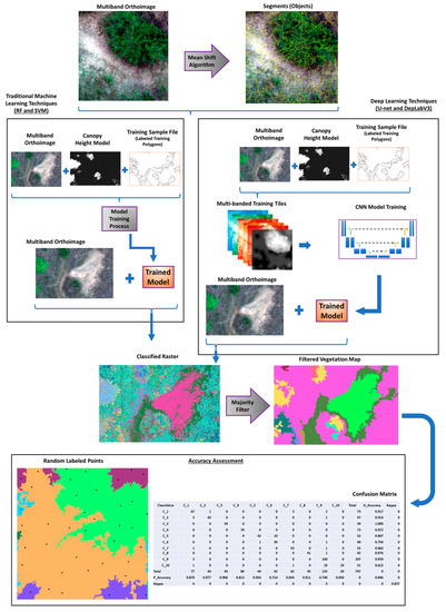
Figure 1.
Workflow recommended in this paper for traditional machine learning techniques and deep learning algorithms.
2.1. Study Area
This study was conducted on an eight-acre, tidally influenced stretch in the Wolf Branch Creek Coastal Nature Preserve, located in West Florida approximately at latitude: 27°44′40.9′′N and longitude: 82°26′34.5′′W, Figure 2. The preserve comprises different types of coastal land cover types, such as upland cabbage palm hammocks, wet and dry grasslands, mangals, and pine flatwoods, where many of those habitats have already been artificially restored. The study area is also affected by the non-native invasive species Brazilian Peppertree (Schinus terebinthifolia), leucaena (Leucaena leucocephala), and cogongrass (Imperata cylindrica), being the last species listed among the top 10 most pervasive exotic invasive plants in the world [61]. The preserve periodically goes through management campaigns to control invasive plant infestations. There are mangrove species, Figure 3, and native grass species, Figure 4, in the study area. Healthy and treated cogongrass is present at the site, Figure 5. A land cover classification schema involving 17 coastal land cover types, Table 1, was adopted. The classes include seven grass species (six natives and one invasive), Cabbage Palmetto (Sabal Palmetto), two mangrove species (Avicennia germinans and Rhizophora mangle), black mangrove (Avicennia germinans), two invasive brush tree species (Brazilian Peppertree (Schinus terebinthifolia), leucaena (Leucaena leucocephala)), water, dead vegetation, and two exposed soil classes, Table 1. The reserve site is actively managed to control and eradicate invasive plants (Brazilian Peppertree sprouts, leucaena, and cogongrass), so we also have a dead vegetation class.
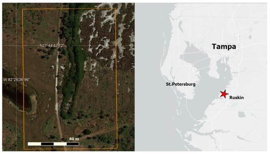
Figure 2.
Study site, located at Wolf Branch creek coastal nature preserve in West Florida.
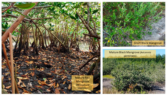
Figure 3.
Mangrove species in the area and black short mangrove.
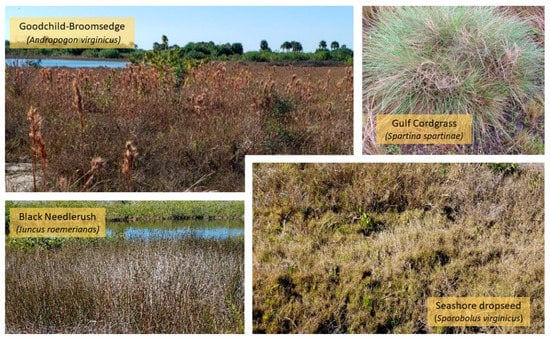
Figure 4.
Native grass species naturally occurring as well as used in coastal restoration.
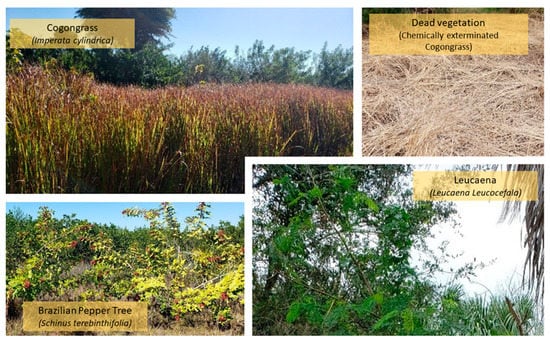
Figure 5.
Invasive species present in the Wolf Branch Creek nature reserve.

Table 1.
Classes defined for the study.
2.2. Field Data Acquisition
Ground Control Point Establishment: In preparation for the UAS data acquisition missions, a set of twelve ground control points (GCP) were established in the study area, Figure 6. The points were surveyed using survey-grade Topcon HiperLite Plus Global Navigation Satellite System (GNSS) receivers with a reported accuracy for a static survey of 3 mm + 0.5 ppm horizontal and 5 mm + 0.5 ppm vertical [63]. A set of three receivers capable of processing signals from the GPS and GLONASS constellations with multipath mitigation were used to occupy each GCP for at least 2 h, collecting measurements every 5 s, Figure 6. The collected GNSS observations were processed using the National Oceanic and Atmospheric Administration’s (NOAA) Online Positioning User Service Projects (OPUS Projects) (https://www.ngs.noaa.gov/OPUS-Projects/OpusProjects.shtml), (accessed on 8 July 2022) to produce control point coordinates with an uncertainty below the centimeter level.
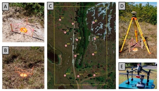
Figure 6.
Study area preparation and data collection (A,B) Ground control points close up views, (C) Ground control points distribution within the study area, enumerated from M1 to M12, (D) GNSS survey, receiver occupying a ground control point, (E) Micasense RedEdge-MX sensor mounted on the “Inspire 2” UAS.
Multispectral Image Acquisition: A Micasense RedEdge-MX multispectral camera capable of acquiring five-band images was mounted on a DJI Inspire 2 (a multi-rotor UAS) and used to acquire the images analyzed in this study, Table 2. The spectral bandwidth, Table 3, and the central wavelength for each of the five bands that were used and the Micasense-MX camera features, Table 4. The UAS was equipped with a Downwelling Light Sensor (DLS) to measure the downwelling irradiance for every image spectral band at the time of acquisition. The DLS is mounted on top of the UAS, pointing toward the sky, Figure 6E. The irradiance value measured at the time each image is acquired is saved in the image metadata and is subsequently retrieved and applied to correct the images. The coordinates of each GCP are used to assure the creation of accurate photogrammetric products with the smallest possible local distortions.
Table 2.
UAS Mission parameters.
Table 3.
Spectral bands in which the MicaSense RedEdge multispectral camera operates (courtesy of www.micasense.com, accessed on 8 July 2022).
Table 4.
MicaSense RedEdge multispectral camera specifications (courtesy of www.micasense.com, accessed on 8 July 2022).
Lidar Data Acquisition: lidar data was collected using a Phoenix Lidar Systems Scout-32 mounted on a DJI M600 UAS. The sensor is made of a combination of a Sony Alpha ILCE-A6000 CMOS 24-megapixel RGB camera and a Velodyne HDL-32E laser scanner and can collect survey-grade data while flying at an altitude of up to 65 m above ground level. The Velodyne HDL-32E sensor is composed of 32 laser range finders arranged in such a way as to be able to cover a 41.33° vertical field of view along the flight direction when mounted on the UAS, Table 5. The UAS measures up to 2 returns per pulse emitted and can record dual returns for objects spaced by at least 1 m [64]. This laser scanner generates a relatively dense cloud of points, acquiring a point cloud of 46,090,005 points covering an area of 32,375 m2 (approximately 8 acres), for an average lidar point density of approximately 1400 points m−2. Two pyramid-shaped targets [65] and two flat targets with highly contrasted patterns were positioned in the study area and located using an RTK GNSS survey to assess lidar data processing accuracy.
Table 5.
Mission and UAS-mounted lidar sensor parameters, courtesy of Velodyne lidar, Inc.
2.3. Preprocessing of Image and lidar Datasets
The multispectral aerial images were processed using a structure from motion (SfM) technique using the Agisoft Metashape software (version 1.7.2 build 12070, St. Petersburg, Russia) [66] to create an orthomosaic with the five spectral bands of the study site. SfM is a computer vision technique that employs series of overlapping images, taken in sequence from different viewpoints, and a highly redundant bundle adjustment to estimate the 3D structure of a scene [67]. The bundle-block adjustment process calculates the coordinates of the ground features in object space as well as the geographic position and orientation of the camera using matched features detected by the algorithm in each sequential image, which are commonly called key points [68]. The GCP coordinates and the geolocation metadata of each image are used to solve the over-constrained optimization process and ultimately transform the image pixel coordinates into a geographic or projected coordinate system.
The 3 cm per pixel resolution orthorectified image mosaic was generated and was free from perspective distortions associated with camera tilts and feature relief, Figure 7. Agisoft also produces a dense, three-dimensional point cloud that represents the features in the scene. The point cloud processing is performed by first running a dense image matching process to identify conjugate image locations within the scene and then by using the image exterior orientation parameters to generate points with real-world X, Y, and Z coordinates [69]. The point cloud was later used to produce a 6 cm DSM to be used in the analyses.
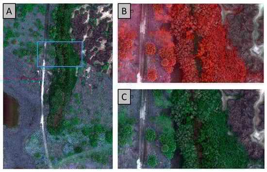
Figure 7.
Study area UAS imagery. (A) Natural color visualization of the study area; the area demarcated by a blue rectangle is displayed in (B,C), (B) Zoomed-in color infrared visualization of area demarcated in (A), (C) Zoomed-in natural color visualization of the demarcated area in (A).
The navigation data of the lidar mission trajectory was analyzed using the Novatel Inertial Explorer software [70]. The highly accurate trajectory solution was then transferred to the Phoenix Lidar Spatial Explorer software [71] to produce a georeferenced point cloud. The georeferenced point cloud was processed using the LAStools software [72] and the function “lasnoise” to reduce noise. Noisy points were filtered out by removing all points without at least 10 other neighboring points within 1 m3, resulting in a cloud averaging 1400 points m−2. Finally, the points were classified as ground and non-ground points using the “lasground” algorithm implemented in the LASTools software [72]. Ten cm pixel size DSM and DTM models were created using the Global Mapper software (version 23.01) [73]. Subtracting the DTM from the DSM results in a CHM that was used as an additional layer (UAS_CHM) in the classification process.
A second CHM was created by combining the following two sources of data: the DSM generated by processing the UAS-acquired multispectral images and the DTM produced from already existing airborne lidar data acquired in 2017 and published by the Southwest Florida Water Management District (SWFWMD) [74]. The airborne topographic lidar data was collected by Dewberry [74] in 2017 using a dual-channel airborne mapping system Riegl VQ-1560i sensor capturing more than 1.3 million measurements per second, flying at an altitude of 1300 m above the ground, with 60 percent overlap. A DTM of 75 cm per pixel was created using this airborne lidar dataset with a mean point density of 16-point m−2. Subsequently, using Global Mapper, this DTM was subtracted from the 6 cm DSM created from the SfM of our multispectral images. The resulting CHM (AB-CHM) was resampled using ArcGIS Pro to reach a resolution of 3 cm per pixel.
2.4. Band Combinations
Three different experiments on data combinations were conducted in this study, Table 6. Experiment 1 tested a set of six spectral band combinations, while experiments 2 and 3 used the same spectral band combinations as experiment 1 plus the canopy height models extracted from UAS-lidar DSM (experiment 2) and image-based DSM (experiment 3), Table 7. It should be noted here that the second experiment was designed to use the following two digital products from less expensive sources: a DTM from the publicly accessible lidar dataset directed by the Southwest Florida Water Management District (SWFWMD) in 2017 and a DSM from the Agisoft Metashape SfM analysis created by processing our UAS-acquired multispectral images as indicated in the previous section.
Table 6.
Experiments, description.
Table 7.
Spectral band combinations studied.
2.5. Training Dataset Preparation
The segment mean shift (SMS) algorithm [75] implemented using the ArcGIS Pro software [66] was applied to the RGB composite of the study site image. The SMS algorithm was used to identify likely objects in the image by clustering together neighboring pixels with similar spectral and spatial characteristics. These three segmentation parameters were tested, namely, spectral detail, spatial detail, and minimum size in pixels, which were simultaneously adjusted until a reasonable object size of 3 m2 was agreed on and used to control the size of the polygons. A total of 24,298 objects covering the whole image were produced, and a group of 3094 objects or polygons (around 180 per land cover type) were randomly selected and manually labeled to train the classifiers. The polygons were labeled as a specific class based on their dominant species, Figure 8. Labeling was conducted in the lab and verified through site visits in collaboration with the Wolf Branch Nature Preserve manager. The same segmentation results were also used to post-process the pixel-based classification by labeling each object with the class to which the majority of its pixels are classified.
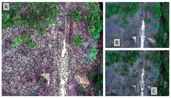
Figure 8.
Image segmentation results (A) polygons delimitating the segmented objects (B) RGB orthoimage, (C) polygons used as training samples during the model training process.
Training data was extracted for every band combination, Table 6. The 3094 training sample polygons were used to train the RF and SVM algorithms (see next section). The same training polygons were used to create training tiles (256 × 256 pixels) from the images with a 128-pixel stride and 30° rotation angles to train the deep learning networks (U-Net and DeepLabv3, see next section), Figure 9. The stride and rotation features were used to augment the training data. Training tiles were only retained for the instances where the polygons and tiles overlapped, resulting in a final set of 27,948 training tiles.
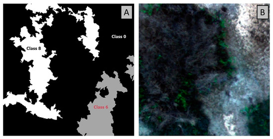
Figure 9.
Training tiles (A) mask showing the three classes identified and labeled in (B) the sample image tile. Class 0 represents the background.
2.6. Data Training and Classification
The U-Net [76] and DeepLabv3 [77] CNN deep learning architectures, widely used for semantic segmentation in the remote sensing community [78,79,80,81], as well as the support vector machine (SVM) [82], and random forest (RF) [83], machine learning algorithms were trained and tested using the same training polygons and accuracy assessment points for all the classifiers used in this study. Training and classification were performed using the ArcGIS Pro software on a computer machine with an Intel(R) Core (TM) i9-10900KF CPU, running at 3.70 GHz with an NVIDIA Titan X 12 GB GPU and 64 GB RAM. The following briefly introduces the classification techniques used in this study.
- Machine Learning Classifiers:
The Random Forest (RF) classifier [84,85] is a decision tree algorithm that applies the most probable class label to each pixel in an image using a set of rules developed during the training process. This process relies on previously labeled training data, where the RF algorithm chooses features and observations randomly to build numerous, uncorrelated decision trees. The final output of the random forest system is formed by the output chosen by the majority of the decision trees. This algorithm is found to be adaptable, fast, simple, the least demanding in terms of computer resources, and a practical machine learning algorithm that generally produces quality outcomes with only a few parameters. After initial experimentation with different parameters, our study adopted a maximum number of trees equal to 50, a maximum tree depth equal to 30 rules (or splits), and a maximum number of samples per class equal to 1000 to be used in the training process. Applying the “Train Random Trees Classifier” from the ArcGIS Pro Image Analyst Toolbox, RF models were trained using the previously labeled training polygons as input training features. The trained model for each band combination was applied to perform pixel classification on the respective raster file using the tool “Classify Raster”, of the ArcGIS Pro, Image Analyst Toolbox.
Support Vector Machine (SVM) is another machine learning algorithm that functions by identifying the hyperplane that best segregates the close observations that belong to separate classes [86,87]. For well-defined and properly labeled classes, the quantity of observations needed to train an SVM classifier is relatively small, yielding reasonably good outcomes compared to more data-demanding algorithms such as CNN [33,88]. This algorithm was applied similarly to the random forest machine learning technique in ArcGIS Pro. The tool “Train Support Vector Machine Classifier” from the ArcGIS Pro Image Analyst Toolbox was employed using the labeled training polygons as input, and the tool “Classify Raster” from the ArcGIS Pro Image Analyst Toolbox was used to classify the rasters after the models were generated.
- Deep Learning Architectures:
The U-Net architecture was introduced in 2015 for biomedical image segmentation at the Computer Science Department of the University of Freiburg to segment cell images [76]. This architecture was designed to minimize the need for classified training data by using the labeled samples more efficiently. The U-Net architecture involves the following two paths: a contracting and an expanding path. The contracting path captures the context within the sample images by applying a sequence of convolution operations and ‘maxpool’ down-sampling to encode the input training images into feature representations. The expanding path allows for accurate localization of each pixel in the image while assigning it a class type. The expanding path uses repeated up-sampling operators that combine high-resolution elements from the contracting path with the up-sampled output, propagating context information to higher resolution layers [76,89].
To train the U-Net architecture, the algorithm was set to balance the classes and ignore the background class. Balancing the classes works by under-sampling the training data from the most numerous classes to pair them down to match the less-represented classes in the dataset. The use of class balancing in the training is intended to avoid biasing the classifier, which would accentuate the most represented class, leading to skewing the classifier decision boundary and producing overfitting [90,91]. Initially, in our study, different training rates were experimented with, and based on those trials, training rates ranging between and were used to train the deep learning models. Similarly, a different number of epochs were tested, and the results revealed that 25 epochs were an adequate amount to train the network in most cases. We used a batch size of 8 in most of our training. These parameters were applied to both deep learning architectures (U-Net and DeepLabV3) used in this study.
DeepLab Version 3: [77] DeepLab is the abbreviation for deep labeling, which is a CNN model for general, dense pixel labeling using deep neural network algorithms. One major challenge when using fully convolutional networks for image classification is that input feature maps become smaller while moving through the convolutional and pooling layers of the network, causing a loss of information contained within the images. Another drawback of the down-sampling performed by the pooling layers in convolutional networks is the lower spatial resolution of the output and blurred object boundaries. DeepLab corrects those pitfalls by removing the down-sampling operations from the last few max-pooling layers of the convolutional network, using atrous convolution [77], and instead using up-sampling in subsequent convolutional layers. The application of this technique results in feature maps processed at a higher sampling rate [92,93].
The backbone for the two deep learning architectures was fixed to ResNet34 [94] due to its powerful performance with reasonable computational power and processing time demands [95]. Although a different number of training epochs were tested, we found that training results often stopped improving after 20 epochs; thus, 25 epochs were used for most of the tested models, which took from 9 to 12 h. The pixel-based classification was then applied using the trained models for each band combination.
2.7. Post-Classification Filtering and Accuracy Assessment
A majority filter was applied to each classified output using the segmented objects initially generated by applying the segment mean shift algorithm [96] to improve the quality of the final classified image through dominant class assignment, Figure 10.
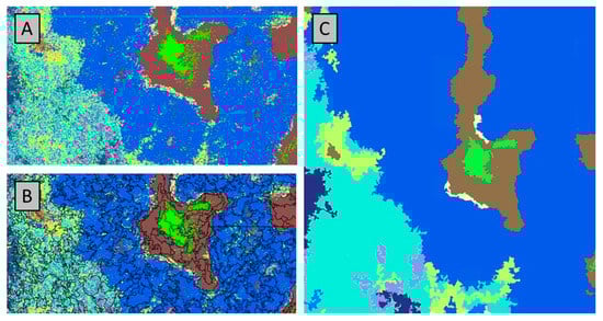
Figure 10.
Majority filter applied to a classified image. (A) Classified image before filtering. (B) Segmented objects used to apply the majority filter. (C) Filtered image produced by labeling each object by its majority class.
An accuracy assessment was conducted on each classified image. A total of 747 random points were created, representing all 17 classes. The points were manually labeled with their corresponding ground truth classes collected through onscreen inspection and field verification. A confusion matrix (error matrix) [97] was created using the randomly generated accuracy assessment points. For each classification result, the overall accuracy (Equation (1)), user accuracy (Equation (2)), producer accuracy (Equation (3)), and the F1-score (Equation (4)) were calculated [98,99,100].
3. Results
3.1. Overall Accuracy
A quantitative evaluation was conducted on the classification experiment results both from using different combinations of five spectral bands (Blue: B, Green: G, Red: R, Near InfraRed: NIR, and RedEdge: RE) in experiment 1 and when adding two canopy height bands (based on SfM solution: AB-CHM for experiment 2 and UAS lidar: UAS-CHM for experiment 3). Four different classifiers (SVM, RF, DeepLabv3, and U-net) were tested in each dataset. In general, the U-net and DeepLabv3 deep learning models require more than 24 h to train a single model. The SVM models were trained for an average of 2 h each, while the RF models only needed an average of 4 min to train. The classification time using a trained deep learning model usually took from one to two minutes, utilizing the GPU to accelerate the process. Classification using RF and SVM did not use the GPU to run the process. RF classifiers needed 3 min, while SVM required between 25 and 40 min.
The same randomly selected accuracy assessment points were used to compute the confusion matrices for all 72 (3 experiments × 6 band combinations × 4 classification techniques) image classifications conducted in this study. The highest accuracy levels achieved by the classification algorithms for the three experiments in the twelve combinations are shown in Figure 11. The user and producer accuracy for each experiment is shown in Appendix A.1, Appendix A.2 and Appendix A.3. The confusion matrices of the trials corresponding to those maps are shown in Appendix B.1, Appendix B.2 and Appendix B.3. The overall accuracy of all tested classifications is shown in Figure 12, and the F1 score is shown in Figure 13 and Figure 14.
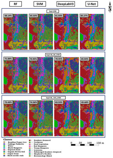
Figure 11.
Vegetation maps corresponding to the highest overall accuracies achieved by each of the four classification algorithms for each experiment.
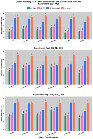
Figure 12.
Overall accuracy of all conducted trials.
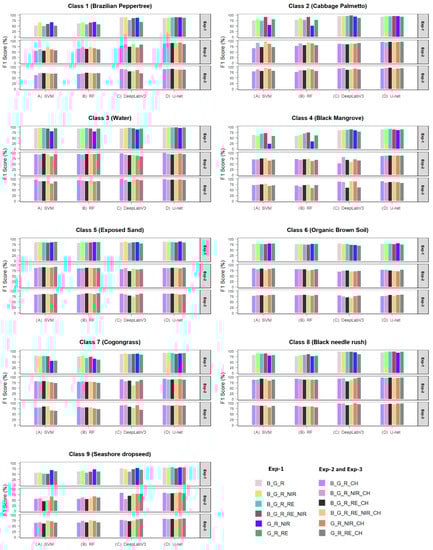
Figure 13.
F1 scores organized by experiment, classification method, and band combination, classes 1 to 9.
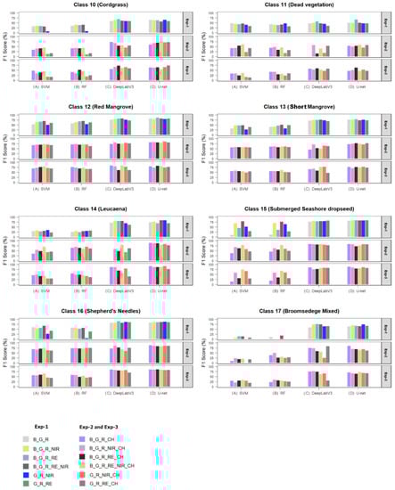
Figure 14.
F1 scores organized by experiment, classification method and band combination, classes 10 to 17.
Deep learning algorithms, especially U-Net, provided higher overall accuracies compared with the RF and SVM traditional machine learning classifiers, Figure 12, which confirms the findings of several other studies, e.g., Liu Tao et al. 2018 [33], Bhatnagar et al. 2020 [101], and Jozdani et al. For example, U-net’s overall accuracy was more than 83.40% in the first experiment for all band combinations, with a maximum of 85.27% for the B_G_R_RE band combination. This contrasts with the 62.65% overall accuracy obtained by RF applied to the same band combination. Similarly, U-net produced overall accuracies in the range of 83.00% to 85.94% in the second and third experiments, compared to SVM yielding accuracies in the range of 62.92% to 74.56% and RF yielding accuracies ranging from 67.07% to 71.89%.
Adding the near-infrared and red edge bands did not seem to have a consistent effect on the overall accuracy of the two deep learning algorithms, Figure 12, which corroborates the findings of other studies, e.g., Li et al. 2021 [102], Zhao et al. 2018 [103]. Including at least one of the near-infrared or red edge bands had a positive influence on the RF and SVM classifiers. This could be explained by the deep learning architecture’s ability to extract and model the important features in a smaller spectral subset, reducing the need for the relatively more expensive multispectral datasets.
Our research matched the findings of other studies [30,104,105], indicating that classes with contrasting spectral properties such as the cabbage palmetto class (class 2), the exposed sand class (class 5), and the black needle rush class (class 8) are in general more likely to be correctly identified by the classifiers (high producer accuracy) and to be reliably mapped (high user accuracy). On the other hand, classes such as the Brazilian pepper tree class (class 1), cordgrass class (class 10), leucaena class (class 14), and submerged seashore dropseed class (class 15), which have similar spectral signatures to other existing classes, have a much higher likelihood of being correctly classified using the deep learning methods than by traditional machine learning classifiers, Figure 13 and Figure 14. All of the classification algorithms, including deep learning, yielded relatively low user accuracies compared to their producer accuracies for the cordgrass class (class 10), leucaena class (class 14), and submerged seashore dropseed class (class 15); Figure 14, (for more detail see Appendix A), which, as mentioned above, have similar spectral signatures to other existing classes. This indicates a higher level of difficulty for those classes to be differentiated when they do not grow isolated from other vegetation species.
In general, the use of the red edge and near-infrared bands in the three experiments yielded slightly higher accuracies in mapping the Brazilian pepper class (class 1), Cabbage palmetto class (class 2), black mangrove class (class 4), organic brown soil class (6), black needle rush class (class 8), cordgrass class (class 10), red mangrove class (class 12), short mangrove class (13), and submerged seashore dropseed (class 15), which could be an argument to consider these bands when those particular land cover types are of interest and need to be mapped using the RF or SVM classifiers Figure 13 and Figure 14, (for more detail see Appendix A). We observed levels of class mixing among classes with similar spectral characteristics in the visible spectrum. For example, the RF and SVM classifiers show the broomsedge class (class 17) was frequently confused with the cogongrass class (class 7), seashore dropseed class (class 9), cordgrass class (class 10), dead vegetation class (class 11), and the Shepherd’s needles class (class 16) (Appendix B). The misclassification is so severe that the user and producer accuracies (Appendix A.1) of these classes in most cases were very low when the RF and SVM classifiers were used. This inability to isolate class 17 did not replicate itself in the deep learning classifications, where U-net was able to map class 17 with an F1 score of around 70%, Figure 14.
3.2. Effect of Canopy Height Models
When comparing the first experiment that used spectral data only with the results of the second and third experiments, we found that using canopy height as a means to incorporate geometrical information in the classification process did not consistently improve the classification accuracy for the deep learning results, Figure 12. This contrasted with the results of the SVM and RF classifiers, which benefited from the extra CHM information. Our results show that the first experiment produced an overall accuracy ranging from 57.43 to 65.33% for the SVM classifier. The overall accuracy improved to a range of 64.79% to 74.56% when the canopy height model was added in experiment 3. The Random Forest increased its accuracy from a range of 60.91% to 68.14% using the spectral bands only to a higher accuracy range of 67.7% to 74.6% when the canopy height model was included in experiment 3.
In general, the CHM obtained from the UAS lidar dataset had a better effect on the overall accuracy of the maps produced by the DeepLabv3 compared to the U-net results, Figure 12. DeepLabV3 achieved slightly higher overall accuracies in the third experiment for all the band combinations except for the G_R_RE_CH band combination. A clear example of this behavior is the band combination of B_G_R_CH, for which DeepLabV3 achieved only 75.4% overall accuracy in the second experiment, where the CHM was produced from SfM and low-resolution DTM was used, and 83.5% overall accuracy in the third experiment using the UAS-based CHM.
For classes with zero canopy height, such as the water class (class 3) and the exposed sand class (class 5), the performance of the deep learning algorithms did not seem to benefit from the addition of the canopy height model, probably due to their distinct spectral characteristics, which prompted higher accuracy outcomes even from the spectral data alone. Individual class performance reflects little to no improvement in the overall accuracy of the deep learning classifications compared to the more substantial improvement in the RF and SVM classification results when canopy heights were introduced. The introduction of the canopy heights improved the accuracy of the SVM and RF classification of the broomsedge class (class 17) noticeably, although the F1 score never reached the 50% mark. The deep learning algorithms, however, probably benefited from the structural and textural differences among the broomsedge and the other grasses, minimizing the influence of the canopy height on the classification process [106,107].
The Shepherd’s needles class (class 16) is another class where RF and SVM benefited from the use of canopy heights with minimal improvement in the accuracy of the deep learning classifiers, Figure 14. The producer accuracy of the SVM results increased from an average of nearly 52% accuracy in the first experiment to about 85% in experiment 2 utilizing (SfM/low-resolution DTM) canopy heights (Appendix A.1). The user accuracy did not improve as much, with an F1 score increasing from an average of 51% to about 56%. The RF classification showed marked improvement, with average producer accuracy growing from 38% to 83% and the user accuracy from 57% to 65%, Figure 13 and Figure 14. It should be noted that this class (class 16) was developed to represent several heavily mixed bushy vegetation species with no apparent dominance of a single species and with relatively similar spectral characteristics and canopy height values.
The introduction of canopy height information in experiments 2 and 3 had a negative effect on the classification accuracy for dead vegetation (class 11). This class represents areas where grass has been either chemically exterminated or bushes mechanically harvested (mulched), and thus, the area would have low canopy height values. When dead vegetation was classified using the spectral bands only, the results were consistent since dead vegetation areas still have consistent and distinguished spectral characteristics. Introducing the canopy heights confused the classifier since dead vegetation had inconsistent canopy height across the landscape. For example, dead but still standing grasses that had been recently chemically treated can have a different height than piles of cut-down tree branches that have not been mulched yet, Figure 14.
3.3. Invasive Plants Classification
Out of the three invasive species (Brazilian pepper, leucaena, and cogongrass) included in our study, the first two have similar spectral signatures, especially when the Brazilian pepper tree is stressed [108,109,110,111]. Healthy Brazilian pepper trees commonly have a dark green appearance, which is not similar to the healthy bright green appearance of leucaena. On the contrary, Brazilian pepper trees growing in coastal wetlands with roots constantly subjected to salt and brackish water inundation typically have leaves that have turned yellowish, making them look much more similar to the natural leucaena color [110]. For all experiments, RF, SVM, and DeepLabV3 showed a predisposition for Brazilian pepper to be confused with leucaena (high omission error), compared to the rest of the vegetation classes. This tendency is less prominent when U-net is used, with U-net more able to identify Brazilian peppers in almost all experiments better. Brazilian pepper (class 1) is often confused with other classes as well, including cabbage palmetto (class 2), black mangrove (class 4), cogongrass (class 7), and seashore dropseed class (class 9) (Appendix B).
The leucaena class (class 14) shows a high producer accuracy, in many cases, close to 100% for all three experiments (Appendix A.1, Appendix A.2 and Appendix A.3) and most of the band combinations of the deep learning classifications, except for two band combinations in trials using DeepLabV3. User accuracy, however, was frequently below 70% for the deep learning results and averaging 32% for the SVM and RF classifiers. The introduction of canopy heights, in all cases, slightly improved the user accuracy of the leucaena class in all tested models. Leucaena prefers elevated dry areas and grows next to grasses such as the seashore dropseed grass, which may explain the positive effect of introducing canopy heights.
When spatially isolated from other grasses, cogongrass was identified by all the classifiers with relatively high accuracy, Figure 13, even as several other grass species with similar spectral properties existed in the study area. Cogongrass was slightly confused with neighboring patches of other grasses when mixed with different grass types in the area. The deep learning algorithms were able to achieve the highest cogongrass classification results among all tested classifiers, Figure A2 in Appendix A. The inclusion of canopy height did not seem to benefit the deep learning classifiers, although RF and SVM showed accuracy improvement. The cogongrass class was not clearly defined by any spectral band combination.
4. Discussion
We found the U-net and DeepLabv3 deep learning networks to be superior compared to the SVM and RF traditional machine learning techniques, which matches the findings of other studies reporting similar ranges of overall accuracy [33,101]. Even though deep learning requires GPUs to train the models in a considerable amount of time, the quality of the achieved results justifies its use when there is no need for expediency, and higher accuracy mapping levels are required.
In this study, we experimented with a relatively large number of coastal land cover classes (17 classes), achieving an overall accuracy higher than 83% using deep learning networks. Previous studies have found similar or comparatively higher values of overall accuracy, although in most of the reviewed cases the number of classes tested has been smaller, either because the studies focused on identifying a single vegetation species or a reduced number of classes [112,113,114]. The outcomes of this research suggest further investigation to explore the possibility of increasing the number of classes and experimenting with different training data sizes to train the machine and deep learning models. Traditional machine learning techniques have reached results comparable to the ones achieved by those techniques in previous studies, e.g., Durgan et al. 2020 [115], highlighting the effectiveness of their use for wetland vegetation mapping using multispectral UAS-acquired datasets.
Adding the near-infrared and red edge spectral bands and the canopy heights improved the accuracy of RF and SVM classifications, while incorporating these additional datasets had minimal, inconsistent impacts on the deep learning classifications. This observation may indicate the efficiency of current deep learning networks in extracting and modeling the features in fewer bands and highlights the need for further exploration of new deep learning network architectures capable of fully utilizing additional spectral and canopy height information. The use of the red edge and near-infrared bands in the three experiments yielded slightly higher accuracies in mapping a few classes. Some classes were significantly mixed, especially when the machine learning classifiers were used.
Although deep learning networks require intensive computational power and longer training times compared to traditional machine learning algorithms, the consistent and considerable accuracy increases achieved using the deep learning models, even when only the three visible bands are used, highlight the advantages of these models. The advantage of deep learning models goes beyond accuracy improvement to sensor utilization, highlighting the potential of using only inexpensive, visible band cameras without the need for the more expensive multispectral cameras.
Based on our findings and backed by the results obtained by other studies experimenting with adding geometric data to classification models [115,116], we recommend the use of canopy height models due to their positive impact on the classification accuracy of specific classes within the deep learning experiments and their significant contribution to the increased accuracy of the RF and SVM results. We also found that both canopy height models derived from UAS lidar datasets and the one derived from SfM photogrammetric model and low-resolution DTM (from airborne lidar datasets) yielded almost similar overall accuracy results in most experiments. This latter realization highlights the fact that even though UAS-lidar remains the preferred method to assure canopy penetration, enabling the construction of high-resolution DTM and canopy height models, the use of a digital surface model extracted from the SfM solution of high-resolution UAS imagery and the often-available low-resolution DTM models extracted from low-density airborne lidar can provide a low-cost alternative to costly UAS lidar datasets.
Even though UAS remote sensing data acquisition and processing, as well as machine learning techniques, are already widely used in coastal environmental monitoring, it is still imperative to further explore and expand the boundaries of knowledge in vegetation classification and invasive species detection, especially as UAS datasets become more integrated into natural resource management operations. For example, concerns related to how to more adequately group classes together as communities to improve the accuracy of the learning models and how to improve the training dataset preparation process remain active research subjects. Additionally, our results showed confusion in some classes that could be improved with more consideration of the operational characteristics (e.g., invasive plant control and removal efforts) in the study area. Utilizing the same methods applied in this study, invasive species detection can also be explored at different phenological and physiological stages, vegetation mixes, and treatment stages [115,117,118].
5. Conclusions
In this study, we assessed the potential of two deep learning architectures (i.e., U-net and DeepLabV3) compared to other traditional machine learning algorithms (i.e., SVM and RF) for coastal wetland vegetation and land cover mapping. The study helps expand the knowledge about the effectiveness of the use of high-resolution UAS-acquired lidar and multispectral data in the generation of accurate vegetation maps. The methods experimented with not only help introduce the application of deep learning techniques in vegetation mapping but also introduce the use of alternative, publicly available lidar data to improve the efficiency of traditional machine learning algorithms in vegetation and land cover classification.
Three experiments were conducted, testing different spectral bands in combination with two canopy height models extracted from UAS lidar observations and the combination of structures from the motion digital surface model and existing digital elevation model. Our findings showed that the U-net network yielded the most consistently accurate classification results, followed in order by the DeepLabV3, RF, and SVM. While deep learning proved to have great potential in the field of vegetation mapping, as was demonstrated by the overall accuracy outcomes achieved in our study, traditional machine learning algorithms, especially RF, which produced overall accuracy that is inferior but still reasonable compared to the deep learning models in a very short time, can be a quick alternative.
Our study reached the conclusion that including the red edge and near-infrared bands in addition to the three visible bands (Green–Blue–Red) produced results that were statistically similar to the results obtained using visible bands only when the classification was carried out using the deep learning techniques. This conclusion did not apply to the RF and SVM classification results. Regarding CHM, the results obtained in this study suggest that canopy height models derived from SfM photogrammetric models and low-resolution DTM (from airborne lidar datasets) are a suitable option to add geometrical information to the machine learning classification models. The study found that even when the accuracy increased using the deep learning techniques compared to traditional machine learning algorithms, the deep learning techniques did not seem to use the full potential of the multispectral and CHM data, suggesting a need for improved deep learning algorithms.
Author Contributions
Conceptualization, A.G.-P., A.A.-E., D.J.J. and R.R.C.; Data curation, A.G.-P.; Formal analysis, A.G.-P.; Funding acquisition, A.A.-E. and B.W.; Investigation, A.G.-P., A.A.-E., B.W. and D.J.J.; Methodology, A.G.-P. and A.A.-E.; Project administration, A.A.-E. and B.W.; Resources, A.A.-E. and B.W.; Software, A.A.-E., B.W. and D.J.J.; Supervision, A.A.-E., B.W. and D.J.J.; Visualization, A.G.-P.; Writing—original draft, A.G.-P.; Writing—review & editing, A.A.-E., B.W., D.J.J. and R.R.C. All authors have read and agreed to the published version of the manuscript.
Funding
This work was supported by the United States Department of Commerce—National Oceanic and Atmospheric Administration (NOAA) through The University of Southern Mississippi under the terms of Agreement No. NA18NOS400198.
Data Availability Statement
Data available will be made publicly accessible after the research is concluded. For the moment the means to share the data used for this study have not been defined.
Acknowledgments
Any use of trade, firm, or product names is for descriptive purposes only and does not imply endorsement by the U.S. Government.
Conflicts of Interest
The authors declare no conflict of interest. The funders had no role in the design of the study; in the collection, analyses, or interpretation of data; in the writing of the manuscript; or in the decision to publish the results.
Appendix A
Appendix A.1. Experiment: EXP1-OSB, Producer and User Accuracy Organized by Class and Classification Method
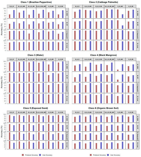
Figure A1.
Experiment: EXP1-OSB, producer and user accuracy organized by class and classification method, classes 1 to 6.
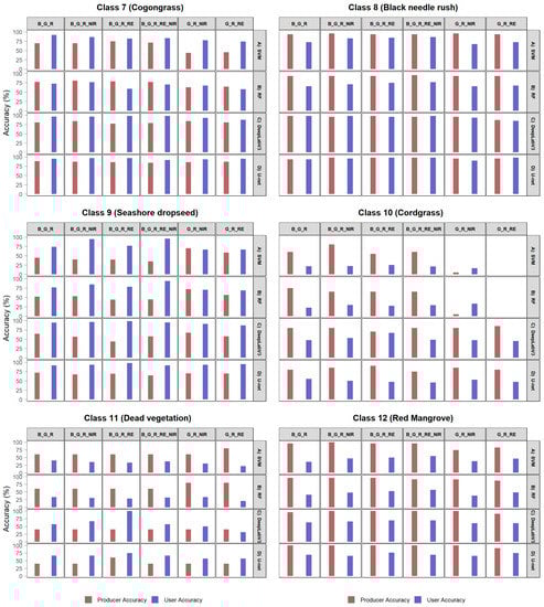
Figure A2.
Experiment: EXP1-OSB, producer and user accuracy organized by class and classification method, classes 7 to 12.
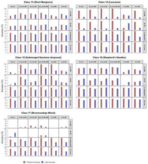
Figure A3.
Experiment: EXP1-OSB, producer and user accuracy organized by class and classification method, classes 13 to 17.
Appendix A.2. Experiment: EXP2-SB_AB_CHM, Producer and User Accuracy Organized by Class and Classification Method
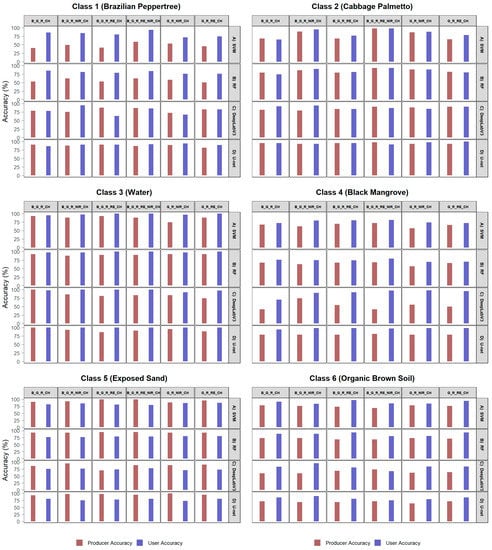
Figure A4.
Experiment: EXP2-SB_AB_CHM, producer and user accuracy organized by class and classification method, classes 1 to 6.
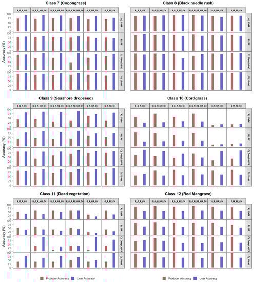
Figure A5.
Experiment: EXP2-SB_AB_CHM, producer and user accuracy organized by class and classification method, classes 7 to 12.
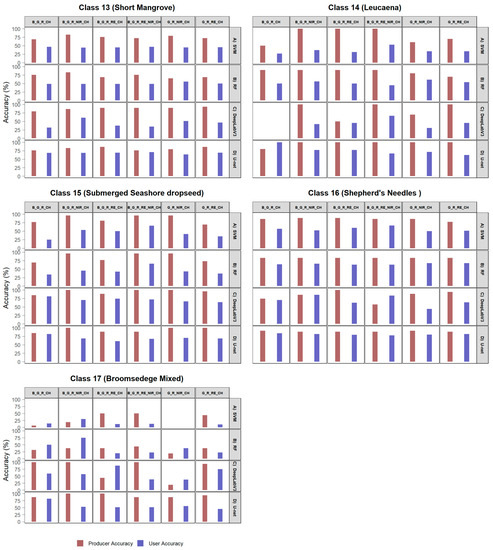
Figure A6.
Experiment: EXP2-SB_AB_CHM, producer and user accuracy organized by class and classification method, classes 13 to 17.
Appendix A.3. Experiment: EXP3-SB_ UAS_CHM, Producer and User Accuracy Organized by Class and Classification Method
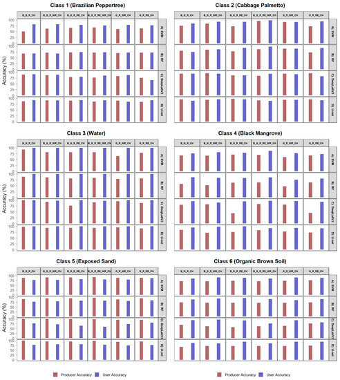
Figure A7.
Experiment: EXP3-SB_ UAS_CHM, producer and user accuracy organized by class and classification method., classes 1 to 6.
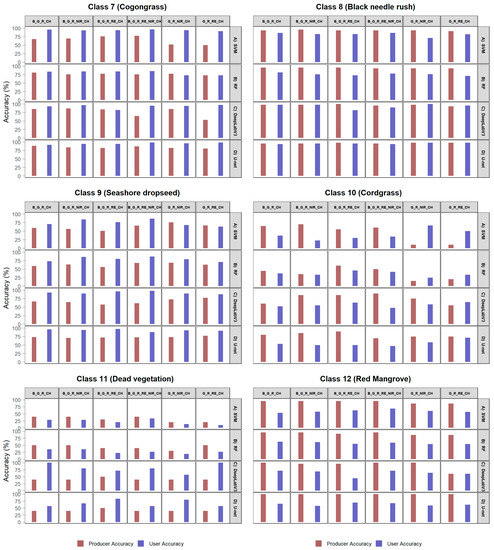
Figure A8.
Experiment: EXP3-SB_ UAS_CHM, producer and user accuracy organized by class and classification method., classes 7 to 12.
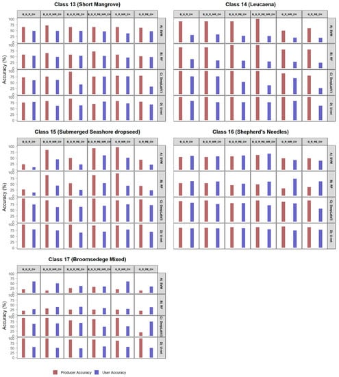
Figure A9.
Experiment: EXP3-SB_ UAS_CHM, producer and user accuracy organized by class and classification method., classes 13 to 17.
Appendix B
Appendix B.1. Confusion Matrices for the Highest Accuracy Results by Classification Method. Experiment 1
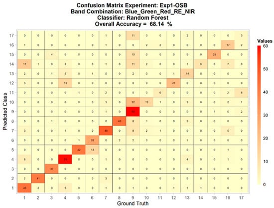
Figure A10.
Confusion matrix for the best results obtained in Exp1-OSB, using the Random Forest classifier (the Blue_Green_Red_RE_NIR band combination).
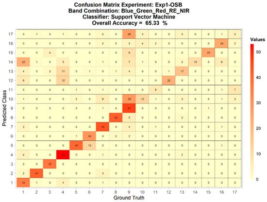
Figure A11.
Confusion matrix for the best results obtained in Exp1-OSB, using the Support Vector Machine classifier (the Blue_Green_Red_RE_NIR band combination).
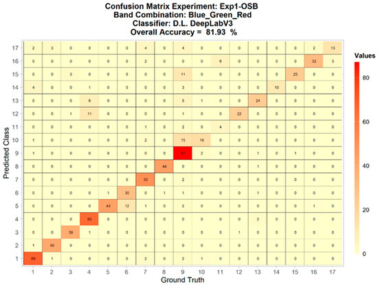
Figure A12.
Confusion matrix for the best results obtained in Exp1-OSB, using the Deep Learning classifier with the DeepLabV3 architecture (the Blue_Green_Red band combination).
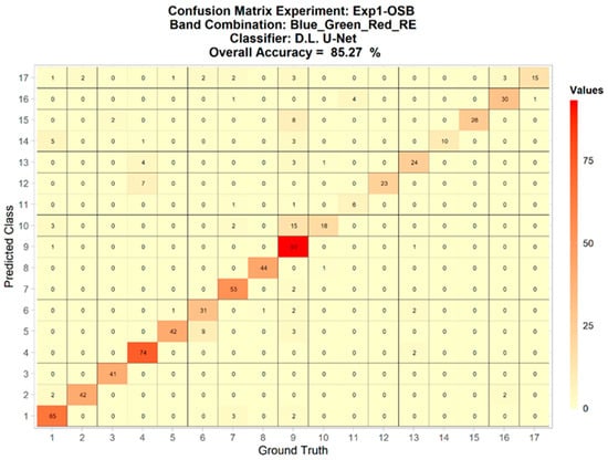
Figure A13.
Confusion matrix for the best results obtained in Exp1-OSB, using the Deep Learning classifier with the U-Net architecture (the Blue_Green_Red_RE band combination).
Appendix B.2. Confusion Matrices for the Highest Accuracy Results by Classification Method. Experiment 2
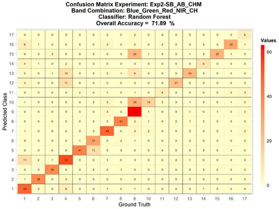
Figure A14.
Confusion matrix for the best results obtained in Exp2-SB_AB_CHM, using the Random Forest classifier (the Blue_Green_Red_NIR_CH band combination).
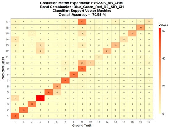
Figure A15.
Confusion matrix for the best results obtained in Exp2-SB_AB_CHM, using the Support Vector Machine classifier (the Blue_Green_Red_RE_NIR_CH band combination).
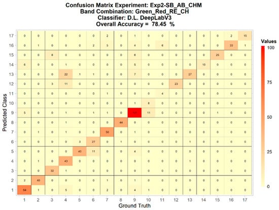
Figure A16.
Confusion matrix for the best results obtained in Exp2-SB_AB_CHM, using the Deep Learning classifier with the DeepLabV3 architecture (the Green_Red_RE_CH band combination).
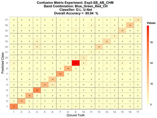
Figure A17.
Confusion matrix for the best results obtained in Exp2-SB_AB_CHM, using the Deep Learning classifier with the U-Net architecture (the Green_Red_RE_CH band combination).
Appendix B.3. Confusion Matrices for the Highest Accuracy Results by Classification Method. Experiment 3
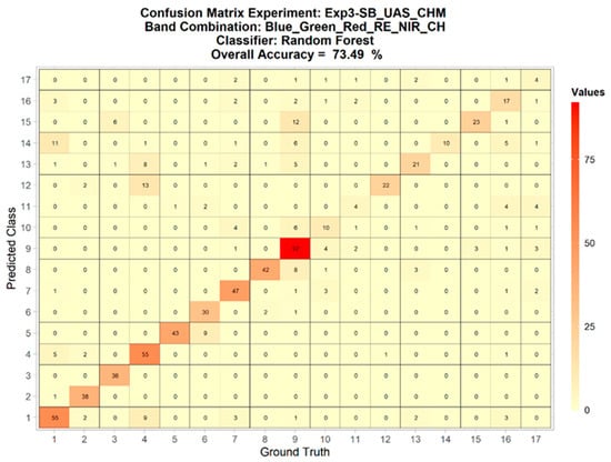
Figure A18.
Confusion matrix for the best results obtained in Exp3-SB_ UAS_CHM, using the Random Forest classifier (the Blue_Green_Red_RE_NIR_CH band combination).
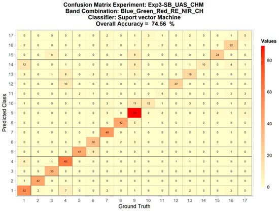
Figure A19.
Confusion matrix for the best results obtained in Exp3-SB_ UAS_CHM, using the Support Vector Machine classifier (the Blue_Green_Red_RE_NIR_CH band combination).
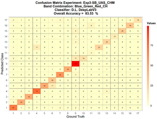
Figure A20.
Confusion matrix for the best results obtained in Exp3-SB_ UAS_CHM, using the DeepLabV3 architecture (the Blue_Green_Red_RE_CH band combination).
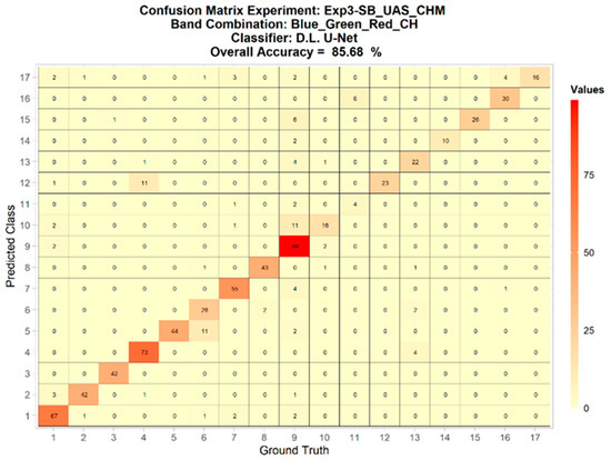
Figure A21.
Confusion matrix for the best results obtained in Exp3-SB_ UAS_CHM, using the Deep Learning classifier with the U-Net architecture (the Blue_Green_Red_CH band combination).
References
- Mendelssohn, I.A.; Byrnes, M.R.; Kneib, R.T.; Vittor, B.A. Coastal Habitats of the Gulf of Mexico. In Habitats and Biota of the Gulf of Mexico: Before the Deepwater Horizon Oil Spill; Springer: New York, NY, USA, 2017; pp. 359–640. [Google Scholar] [CrossRef]
- Lefcheck, J.S.; Hughes, B.B.; Johnson, A.J.; Pfirrmann, B.W.; Rasher, D.B.; Smyth, A.R.; Williams, B.L.; Beck, M.W.; Orth, R.J. Are coastal habitats important nurseries? A meta-analysis. Conserv. Lett. 2019, 12, e12645. [Google Scholar] [CrossRef]
- Florida Department of Environmental Protection. Benefits of Mangroves. 13 April 2022. Available online: https://floridadep.gov/water/submerged-lands-environmental-resources-coordination/content/what-mangrove (accessed on 3 August 2022).
- Elisha, O.D.; Felix, M.J. Destruction of Coastal Ecosystems and The Vicious Cycle of Poverty in Niger Delta Region 2021. Available online: https://www.ikppress.org/index.php/JOGAE/article/view/6602 (accessed on 3 August 2022).
- Kirwan, M.L.; Megonigal, J.P. Tidal wetland stability in the face of human impacts and sea-level rise. Nature 2013, 504, 53–60. [Google Scholar] [CrossRef] [PubMed]
- Van Asselen, P.S.; Verburg, H.; Vermaat, J.E.; Janse, J.H. Drivers of Wetland Conversion: A Global Meta-Analysis. PLoS ONE 2013, 8, e81292. [Google Scholar] [CrossRef] [PubMed]
- Lotze, H.K.; Lenihan, H.S.; Bourque, B.J.; Bradbury, R.H.; Cooke, R.G.; Kay, M.C.; Kidwell, S.M.; Kirby, M.X.; Peterson, C.H.; Jackson, J.B.C. Depletion, Degradation, and Recovery Potential of Estuaries and Coastal Seas. Science 2006, 312, 1806–1809. [Google Scholar] [CrossRef] [PubMed]
- Syvitski, J.P.M.; Vörösmarty, C.J.; Kettner, A.J.; Green, P. Impact of Humans on the Flux of Terrestrial Sediment to the Global Coastal Ocean. Science 2005, 308, 376–380. [Google Scholar] [CrossRef] [PubMed]
- McCarthy, M.J.; Colna, K.E.; El-Mezayen, M.M.; Laureano-Rosario, A.; Méndez-Lázaro, P.; Otis, D.B.; Toro-Farmer, G.; Vega-Rodriguez, M.; Muller-Karger, F.E. Satellite Remote Sensing for Coastal Management: A Review of Successful Applications. Environ. Manag. 2017, 60, 323–339. [Google Scholar] [CrossRef] [PubMed]
- Staver, L.W.; Stevenson, J.C.; Cornwell, J.C.; Nidzieko, N.J.; Owens, M.S.; Logan, L.; Kim, C.; Malkin, S.Y. Tidal Marsh Restoration at Poplar Island: II. Elevation Trends, Vegetation Development, and Carbon Dynamics. Wetlands 2020, 40, 1687–1701. [Google Scholar] [CrossRef]
- Bull, D.; Lim, N.; Frank, E. Perceptual improvements for Super-Resolution of Satellite Imagery. In Proceedings of the 2021 36th International Conference on Image and Vision Computing New Zealand (IVCNZ), Hamilton, New Zealand, 9–10 December 2021; pp. 1–6. [Google Scholar] [CrossRef]
- Gray, P.; Ridge, J.T.; Poulin, S.K.; Seymour, A.C.; Schwantes, A.M.; Swenson, J.J.; Johnston, D.W. Integrating Drone Imagery into High Resolution Satellite Remote Sensing Assessments of Estuarine Environments. Remote Sens. 2018, 10, 1257. [Google Scholar] [CrossRef]
- Jeziorska, J. UAS for Wetland Mapping and Hydrological Modeling. Remote Sens. 2019, 11, 1997. [Google Scholar] [CrossRef]
- Griffin, S.; Lasko, K. Using Unmanned Aircraft System (UAS) and Satellite Imagery to Map Aquatic and Terrestrial Vegetation. 2020. Available online: https://doi.org/10.21079/11681/38086 (accessed on 3 August 2022). [CrossRef]
- Thomas, O.; Stallings, C.; Wilkinson, B. Unmanned aerial vehicles can accurately, reliably, and economically compete with terrestrial mapping methods. J. Unmanned Veh. Syst. 2020, 8, 57–74. [Google Scholar] [CrossRef]
- Addo, K.A.; Jayson-Quashigah, P.-N. UAV photogrammetry and 3D reconstruction: Application in coastal monitoring. In Unmanned Aerial Systems; Elsevier: Amsterdam, The Netherlands, 2021; pp. 157–174. [Google Scholar] [CrossRef]
- Makri, D.; Stamatis, P.; Doukari, M.; Papakonstantinou, A.; Vasilakos, C.; Topouzelis, K. Multi-Scale Seagrass Mapping in Satellite Data and the Use of UAS in Accuracy Assessment. 2018. Available online: https://www.spiedigitallibrary.org/conference-proceedings-of-spie/10773/107731T/Multi-scale-seagrass-mapping-in-satellite-data-and-the-use/10.1117/12.2326012.short (accessed on 3 August 2022).
- Suo, C.; McGovern, E.; Gilmer, A. Coastal Dune Vegetation Mapping Using a Multispectral Sensor Mounted on an UAS. Remote Sens. 2019, 11, 1814. [Google Scholar] [CrossRef]
- Pinton, D.; Canestrelli, A.; Angelini, C.; Wilkinson, B.; Ifju, P. Inferring the Spatial Distribution of Vegetation Height and Density in a Mesotidal Salt Marsh From UAV LIDAR Data. AGU Fall Meeting Abstracts. 2019. Available online: https://ui.adsabs.harvard.edu/abs/2019AGUFMEP11E2069P/abstract (accessed on 3 August 2022).
- Turner, I.L.; Harley, M.D.; Drummond, C.D. UAVs for coastal surveying. Coast. Eng. 2016, 114, 19–24. [Google Scholar] [CrossRef]
- Topouzelis, K.; Papakonstantinou, A.; Pavlogeorgatos, G. Coastline Change Detection Using Uav, Remote Sensing, GIS and 3D Reconstruction. 2015. Available online: https://d1wqtxts1xzle7.cloudfront.net/47781906/Abstract_CEMEPE_2015-with-cover-page-v2.pdf?Expires=1659623181&Signature=AYcxjwH4PeKXeJ3LopMhsWGgVNeIg8l6~ttUCQYXx-9L3GNFJFawP1dlc7gJNxrAogPZbeuX9BsTA~kWVVlIka-Z4tDsy6GXI24TfEwKmEAUfkRoIO-wIZJvY4SV6KNCkai7nQY65TjzdPaL2Xk4O6wwMwm8p8cjqOvEoXVLYQ2s99pYVa3tHXPRbkxXbo9zzmPy7epuk1XurWbQj25M1UKrSkLJo2lvgRvdx8Ye2YJAdepB2-cJQCv5MjnDUJjozRhXo0Css4fBlLjCDufR6FFr-cFOBuDgfzPdUGjivswdJt9z-ddfvjIquENbv6hul4-5qQkj2sF5mK2mIEmY3g__&Key-Pair-Id=APKAJLOHF5GGSLRBV4ZA (accessed on 3 August 2022).
- Mancini, F.; Dubbini, M.; Gattelli, M.; Stecchi, F.; Fabbri, S.; Gabbianelli, G. Using Unmanned Aerial Vehicles (UAV) for High-Resolution Reconstruction of Topography: The Structure from Motion Approach on Coastal Environments. Remote Sens. 2013, 5, 6880–6898. [Google Scholar] [CrossRef]
- Long, N.; Millescamps, B.; Guillot, B.; Pouget, F.; Bertin, X. Monitoring the Topography of a Dynamic Tidal Inlet Using UAV Imagery. Remote Sens. 2016, 8, 387. [Google Scholar] [CrossRef]
- Ventura, D.; Bruno, M.; Lasinio, G.J.; Belluscio, A.; Ardizzone, G. A low-cost drone based application for identifying and mapping of coastal fish nursery grounds. Estuar. Coast. Shelf Sci. 2016, 171, 85–98. [Google Scholar] [CrossRef]
- Casella, E.; Collin, A.; Harris, D.; Ferse, S.; Bejarano, S.; Parravicini, V.; Hench, J.L.; Rovere, A. Mapping coral reefs using consumer-grade drones and structure from motion photogrammetry techniques. Coral Reefs 2017, 36, 269–275. [Google Scholar] [CrossRef]
- Cao, J.; Liu, K.; Zhuo, L.; Liu, L.; Zhu, Y.; Peng, L. Combining UAV-based hyperspectral and LiDAR data for mangrove species classification using the rotation forest algorithm. Int. J. Appl. Earth Obs. Geoinf. 2021, 102, 102414. [Google Scholar] [CrossRef]
- Barbour, T.E.; Sassaman, K.E.; Zambrano, A.M.A.; Broadbent, E.N.; Wilkinson, B.; Kanaski, R. Rare pre-Columbian settlement on the Florida Gulf Coast revealed through high-resolution drone LiDAR. Proc. Natl. Acad. Sci. USA 2019, 116, 23493–23498. [Google Scholar] [CrossRef] [PubMed]
- Pinton, D.; Canestrelli, A.; Wilkinson, B.; Ifju, P.; Ortega, A. A new algorithm for estimating ground elevation and vegetation characteristics in coastal salt marshes from high-resolution UAV-based LiDAR point clouds. Earth Surf. Processes Landf. 2020, 45, 3687–3701. [Google Scholar] [CrossRef]
- Zhu, X.; Meng, L.; Zhang, Y.; Weng, Q.; Morris, J. Tidal and Meteorological Influences on the Growth of Invasive Spartina alterniflora: Evidence from UAV Remote Sensing. Remote Sens. 2019, 11, 1208. [Google Scholar] [CrossRef]
- Abeysinghe, T.; Simic Milas, A.; Arend, K.; Hohman, B.; Reil, P.; Gregory, A.; Vázquez-Ortega, A. Mapping Invasive Phragmites australis in the Old Woman Creek Estuary Using UAV Remote Sensing and Machine Learning Classifiers. Remote Sens. 2019, 11, 1380. [Google Scholar] [CrossRef]
- Baena, S.; Moat, J.; Whaley, O.; Boyd, D.S. Identifying species from the air: UAVs and the very high resolution challenge for plant conservation. PLoS ONE 2017, 12, e0188714. [Google Scholar] [CrossRef] [PubMed]
- Pix4D. Reflectance Map vs Orthomosaic. 2022. Available online: https://support.pix4d.com/hc/en-us/articles/202739409-Reflectance-map-vs-orthomosaic (accessed on 3 August 2022).
- Liu, T.; Abd-Elrahman, A.; Morton, J.; Wilhelm, V.L. Comparing fully convolutional networks, random forest, support vector machine, and patch-based deep convolutional neural networks for object-based wetland mapping using images from small unmanned aircraft system. GIScience Remote Sens. 2018, 55, 243–264. [Google Scholar] [CrossRef]
- Liu, T.; Abd-Elrahman, A. An Object-Based Image Analysis Method for Enhancing Classification of Land Covers Using Fully Convolutional Networks and Multi-View Images of Small Unmanned Aerial System. Remote Sens. 2018, 10, 457. [Google Scholar] [CrossRef]
- Chust, G.; Galparsoro, I.; Borja, Á.; Franco, J.; Uriarte, A. Coastal and estuarine habitat mapping, using LIDAR height and intensity and multi-spectral imagery. Estuar. Coast. Shelf Sci. 2008, 78, 633–643. [Google Scholar] [CrossRef]
- Schmid, K.A.; Hadley, B.C.; Wijekoon, N. Vertical Accuracy and Use of Topographic LIDAR Data in Coastal Marshes. J. Coast. Res. 2011, 275, 116–132. [Google Scholar] [CrossRef]
- Green, D.R.; Gregory, B.J.; Karachok, A.R. Unmanned Aerial Remote Sensing; CRC Press: Boca Raton, FL, USA, 2020. [Google Scholar] [CrossRef]
- Adade, R.; Aibinu, A.M.; Ekumah, B.; Asaana, J. Unmanned Aerial Vehicle (UAV) applications in coastal zone management—A review. Environ. Monit. Assess. 2021, 193, 154. [Google Scholar] [CrossRef]
- Zhu, X.; Hou, Y.; Weng, Q.; Chen, L. Integrating UAV optical imagery and LiDAR data for assessing the spatial relationship between mangrove and inundation across a subtropical estuarine wetland. ISPRS J. Photogramm. Remote Sens. 2019, 149, 146–156. [Google Scholar] [CrossRef]
- Xu, X.; Song, X.; Li, T.; Shi, Z.; Pan, B. Deep Autoencoder for Hyperspectral Unmixing via Global-Local Smoothing. IEEE Trans. Geosci. Remote Sens. 2022, 60, 1–16. [Google Scholar] [CrossRef]
- Sheykhmousa, M.; Mahdianpari, M.; Ghanbari, H.; Mohammadimanesh, F.; Ghamisi, P.; Homayouni, S. Support Vector Machine Versus Random Forest for Remote Sensing Image Classification: A Meta-Analysis and Systematic Review. IEEE J. Sel. Top. Appl. Earth Obs. Remote Sens. 2020, 13, 6308–6325. [Google Scholar] [CrossRef]
- Pan, B.; Qu, Q.; Xu, X.; Shi, Z. Structure–Color Preserving Network for Hyperspectral Image Super-Resolution. IEEE Trans. Geosci. Remote Sens. 2022, 60, 1–12. [Google Scholar] [CrossRef]
- Kwenda, C.; Gwetu, M.; Dombeu, J.V.F. Machine Learning Methods for Forest Image Analysis and Classification: A Survey of the State of the Art. IEEE Access 2022, 10, 45290–45316. [Google Scholar] [CrossRef]
- Koetz, B.; Morsdorf, F.; van der Linden, S.; Curt, T.; Allgöwer, B. Multi-source land cover classification for forest fire management based on imaging spectrometry and LiDAR data. For. Ecol. Manag. 2008, 256, 263–271. [Google Scholar] [CrossRef]
- Gigović, L.; Pourghasemi, H.R.; Drobnjak, S.; Bai, S. Testing a New Ensemble Model Based on SVM and Random Forest in Forest Fire Susceptibility Assessment and Its Mapping in Serbia’s Tara National Park. Forests 2019, 10, 408. [Google Scholar] [CrossRef]
- Ahmad, A.M.; Minallah, N.; Ahmed, N.; Ahmad, A.M.; Fazal, N. Remote Sensing Based Vegetation Classification Using Machine Learning Algorithms. In Proceedings of the 2019 International Conference on Advances in the Emerging Computing Technologies (AECT), Al Madinah Al Munawwarah, Saudi Arabia, 10 February 2020; pp. 1–6. [Google Scholar] [CrossRef]
- Wang, H.; Han, D.; Mu, Y.; Jiang, L.; Yao, X.; Bai, Y.; Lu, Q.; Wang, F. Landscape-level vegetation classification and fractional woody and herbaceous vegetation cover estimation over the dryland ecosystems by unmanned aerial vehicle platform. Agric. For. Meteorol 2019, 278, 107665. [Google Scholar] [CrossRef]
- Ahmed, O.S.; Shemrock, A.; Chabot, D.; Dillon, C.; Williams, G.; Wasson, R.; Franklin, S.E. Hierarchical land cover and vegetation classification using multispectral data acquired from an unmanned aerial vehicle. Int. J. Remote Sens. 2017, 38, 2037–2052. [Google Scholar] [CrossRef]
- Erinjery, J.J.; Singh, M.; Kent, R. Mapping and assessment of vegetation types in the tropical rainforests of the Western Ghats using multispectral Sentinel-2 and SAR Sentinel-1 satellite imagery. Remote Sens. Environ. 2018, 216, 345–354. [Google Scholar] [CrossRef]
- Macintyre, P.D.; van Niekerk, A.; Dobrowolski, M.P.; Tsakalos, J.L.; Mucina, L. Impact of ecological redundancy on the performance of machine learning classifiers in vegetation mapping. Ecol. Evol. 2018, 8, 6728–6737. [Google Scholar] [CrossRef]
- Rommel, E.; Giese, L.; Fricke, K.; Kathöfer, F.; Heuner, M.; Mölter, T.; Deffert, P.; Asgari, M.; Näthe, P.; Dzunic, F.; et al. Very High-Resolution Imagery and Machine Learning for Detailed Mapping of Riparian Vegetation and Substrate Types. Remote Sens. 2022, 14, 954. [Google Scholar] [CrossRef]
- Zagajewski, B.; Kluczek, M.; Raczko, E.; Njegovec, A.; Dabija, A.; Kycko, M. Comparison of Random Forest, Support Vector Machines, and Neural Networks for Post-Disaster Forest Species Mapping of the Krkonoše/Karkonosze Transboundary Biosphere Reserve. Remote Sens. 2021, 13, 2581. [Google Scholar] [CrossRef]
- Uehara, T.D.T.; Corrêa, S.P.L.P.; Quevedo, R.P.; Körting, T.S.; Dutra, L.V.; Rennó, C.D. Landslide Scars Detection using Remote Sensing and Pattern Recognition Techniques: Comparison Among Artificial Neural Networks, Gaussian Maximum Likelihood, Random Forest, and Support Vector Machine Classifiers. Rev. Bras. De Cartogr. 2020, 72, 665–680. Available online: http://www.seer.ufu.br/index.php/revistabrasileiracartografia/article/view/54037/30208 (accessed on 3 August 2022). [CrossRef]
- Alzubaidi, L.; Zhang, J.; Humaidi, A.J.; Al-Dujaili, A.; Duan, Y.; Al-Shamma, O.; Santamaría, J.; Fadhel, M.A.; Al-Amidie, M.; Farhan, L. Review of deep learning: Concepts, CNN architectures, challenges, applications, future directions. J. Big Data 2021, 8, 53. [Google Scholar] [CrossRef] [PubMed]
- Bengio, Y.; Courville, A.; Vincent, P. Representation Learning: A Review and New Perspectives. IEEE Trans. Pattern Anal. Mach. Intell. 2013, 35, 1798–1828. [Google Scholar] [CrossRef]
- Li, B.; Pi, D. Network representation learning: A systematic literature review. Neural Comput. Appl. 2020, 32, 16647–16679. [Google Scholar] [CrossRef]
- Pedergnana, M.; Marpu, P.R.; Mura, M.D.; Benediktsson, J.A.; Bruzzone, L. A Novel Technique for Optimal Feature Selection in Attribute Profiles Based on Genetic Algorithms. IEEE Trans. Geosci. Remote Sens. 2013, 51, 3514–3528. [Google Scholar] [CrossRef]
- Novack, T.; Esch, T.; Kux, H.; Stilla, U. Machine Learning Comparison between WorldView-2 and QuickBird-2-Simulated Imagery Regarding Object-Based Urban Land Cover Classification. Remote Sens. 2011, 3, 2263–2282. [Google Scholar] [CrossRef]
- Topouzelis, K.; Psyllos, A. Oil spill feature selection and classification using decision tree forest on SAR image data. ISPRS J. Photogramm. Remote Sens. 2012, 68, 135–143. [Google Scholar] [CrossRef]
- Melgani, F.; Bruzzone, L. Classification of hyperspectral remote sensing images with support vector machines. IEEE Trans. Geosci. Remote Sens. 2004, 42, 1778–1790. [Google Scholar] [CrossRef]
- Dozier, H.; Gaffney, J.F.; McDonald, S.K.; Johnson, E.R.R.L.; Shilling, D.G. Cogongrass in the United States: History, Ecology, Impacts, and Management. Weed Technol. 1998, 12, 737–743. [Google Scholar] [CrossRef]
- Kauffman, J.B.; Donato, D. Protocols for the Measurement, Monitoring and Reporting of Structure, Biomass and Carbon Stocks in Mangrove Forests. Center for International Forestry Research (CIFOR): Bogor, Indonesia, 2012. [Google Scholar] [CrossRef]
- Topcon Corporation. Hiper Lite +. January 2004. Available online: https://www.lengemann.us/pdf/HiPerLitePlus_Broch_REVC.pdf (accessed on 3 August 2022).
- Velodyne. Velodyne LiDAR HDL-32E User’s Manual. 2021. Available online: https://velodynelidar.com/downloads/ (accessed on 3 August 2022).
- Wilkinson, B.; Lassiter, H.A.; Abd-Elrahman, A.; Carthy, R.R.; Ifju, P.; Broadbent, E.; Grimes, N. Geometric Targets for UAS Lidar. Remote Sens. 2019, 11, 3019. [Google Scholar] [CrossRef]
- Agisoft LLC. Agisoft Metashape User Manual: Professional Edition, Version 1.8. 2022. Available online: https://www.agisoft.com/pdf/metashape-pro_1_8_en.pdf (accessed on 3 August 2022).
- Westoby, M.J.; Brasington, J.; Glasser, N.F.; Hambrey, M.J.; Reynolds, J.M. ‘Structure-from-Motion’ photogrammetry: A low-cost, effective tool for geoscience applications. Geomorphology 2012, 179, 300–314. [Google Scholar] [CrossRef]
- Triggs, B.; McLauchlan, P.F.; Hartley, R.I.; Fitzgibbon, A.W. Bundle Adjustment—A Modern Synthesis. In International Workshop on Vision Algorithms; Springer: Berlin/Heidelberg, Germany, 2000; pp. 298–372. [Google Scholar] [CrossRef]
- Wolf, P.R.; Dewitt, B.A.; Wilkinson, B.E. Elements of Photogrammetry with Applications in GIS, 4th ed.; McGraw-Hill Education: New York, NY, USA, 2014; Available online: https://www.accessengineeringlibrary.com/content/book/9780071761123 (accessed on 3 August 2022).
- Hexagon © 2022. Inertial Explorer®. January 2022. Available online: https://novatel.com/products/waypoint-post-processing-software/inertial-explorer (accessed on 3 August 2022).
- Phoenix LiDAR Systems. Learn about the Latest Spatial Explorer 6.0 Features. January 2021. Available online: https://www.phoenixlidar.com/software/ (accessed on 3 August 2022).
- Rapidlasso GmbH. LAStools-Efficient LiDAR Processing Software. January 2022. Available online: https://rapidlasso.com/LAStools/ (accessed on 3 August 2022).
- Blue Marble Geographics®. Global Mapper Pro®. 2022. Available online: https://www.bluemarblegeo.com/global-mapper-pro/ (accessed on 3 August 2022).
- Dewberry. Dewberry to Collect and Process Lidar Data for Southwest Florida Water Management District. 2021. Available online: https://www.dewberry.com/insights-news/article/2017/05/16/dewberry-to-collect-and-process-lidar-data-for-southwest-florida-water-management-district (accessed on 3 August 2022).
- Fukunaga, K.; Hostetler, L. The estimation of the gradient of a density function, with applications in pattern recognition. IEEE Trans. Inf. Theory 1975, 21, 32–40. [Google Scholar] [CrossRef]
- Ronneberger, O.; Fischer, P.; Brox, T. U-Net: Convolutional Networks for Biomedical Image Segmentation. In Medical Image Computing and Computer-Assisted Intervention 2015; Navab, N., Hornegger, J., Wells, W.M., Frangi, A.F., Eds.; Springer International Publishing: Cham, Switzerland, 2015; pp. 234–241. [Google Scholar] [CrossRef]
- Chen, L.-C.; Papandreou, G.; Kokkinos, I.; Murphy, K.; Yuille, A.L. DeepLab: Semantic Image Segmentation with Deep Convolutional Nets, Atrous Convolution, and Fully Connected CRFs. IEEE Trans. Pattern Anal. Mach. Intell. 2018, 40, 834–848. [Google Scholar] [CrossRef] [PubMed]
- Zhao, H.; Shi, J.; Qi, X.; Wang, X.; Jia, J. Pyramid Scene Parsing Network. In Proceedings of the 2017 IEEE Conference on Computer Vision and Pattern Recognition, Honolulu, HI, USA, 21–26 July 2017. [Google Scholar]
- Heydari, S.S.; Mountrakis, G. Meta-analysis of deep neural networks in remote sensing: A comparative study of mono-temporal classification to support vector machines. ISPRS J. Photogramm. Remote Sens. 2019, 152, 192–210. [Google Scholar] [CrossRef]
- Ma, L.; Liu, Y.; Zhang, X.; Ye, Y.; Yin, G.; Johnson, B.A. Deep learning in remote sensing applications: A meta-analysis and review. ISPRS J. Photogramm. Remote Sens. 2019, 152, 166–177. [Google Scholar] [CrossRef]
- Mohammadimanesh, F.; Salehi, B.; Mahdianpari, M.; Gill, E.; Molinier, M. A new fully convolutional neural network for semantic segmentation of polarimetric SAR imagery in complex land cover ecosystem. ISPRS J. Photogramm. Remote Sens. 2019, 151, 223–236. [Google Scholar] [CrossRef]
- Hsu, C.W.; Chang, C.C.; Lin, C.J. A Practical Guide to Support Vector Classification. 2003. Available online: https://www.csie.ntu.edu.tw/~cjlin/papers/guide/guide.pdf (accessed on 3 August 2022).
- Ponraj, A. Decision Trees. DevSkrol. July 2020. Available online: https://devskrol.com/2020/07/26/random-forest-how-random-forest-works/ (accessed on 3 August 2022).
- Breiman, L. Random Forests. Mach. Learn. 2001, 45, 5–32. [Google Scholar] [CrossRef]
- David, D. Random Forest Classifier Tutorial: How to Use Tree-Based Algorithms for Machine Learning. freeCodeCamp. 2020. Available online: https://www.freecodecamp.org/news/how-to-use-the-tree-based-algorithm-for-machine-learning/ (accessed on 3 August 2022).
- Cortes, C.; Vapnik, V. Support-vector networks. Mach. Learn. 1995, 20, 273–297. [Google Scholar] [CrossRef]
- Hsu, C.-W.; Lin, C.-J. A comparison of methods for multiclass support vector machines. IEEE Trans. Neural Netw. 2002, 13, 415–425. [Google Scholar] [CrossRef]
- Chandra, M.A.; Bedi, S.S. Survey on SVM and their application in image classification. Int. J. Inf. Technol. 2018, 13, 1–11. [Google Scholar] [CrossRef]
- Zhou, Z.; Siddiquee, M.M.R.; Tajbakhsh, N.; Liang, J. UNet++: A Nested U-Net Architecture for Medical Image Segmentation. In Deep Learning in Medical Image Analysis and Multimodal Learning for Clinical Decision Support; Lecture Notes in Computer Science; Springer: Berlin/Heidelberg, Germany, 2018; pp. 3–11. [Google Scholar] [CrossRef]
- Feng, R.; Gu, J.; Qiao, Y.; Dong, C. Suppressing Model Overfitting for Image Super-Resolution Networks. In Proceedings of the IEEE/CVF Conference on Computer Vision and Pattern Recognition Workshops, Long Beach, CA, USA, 16–17 June 2019. [Google Scholar]
- Buda, M.; Maki, A.; Mazurowski, M.A. A systematic study of the class imbalance problem in convolutional neural networks. Neural Netw. 2018, 106, 249–259. [Google Scholar] [CrossRef] [PubMed]
- Tsang, S.-H. Review: DeepLabv3—Atrous Convolution (Semantic Segmentation). Towards Data Science. 19 January 2019. Available online: https://towardsdatascience.com/review-deeplabv3-atrous-convolution-semantic-segmentation-6d818bfd1d74 (accessed on 3 August 2022).
- Chen, L.-C.; Papandreou, G.; Schroff, F.; Adam, H. Rethinking Atrous Convolution for Semantic Image Segmentation. arXiv 2017, arXiv:1706.05587. [Google Scholar]
- He, K.; Zhang, X.; Ren, S.; Sun, J. Deep Residual Learning for Image Recognition. In Proceedings of the 2016 IEEE Conference on Computer Vision and Pattern Recognition (CVPR), Las Vegas, NV, USA, 27–30 June 2016; pp. 770–778. [Google Scholar] [CrossRef]
- Canziani, A.; Paszke, A.; Culurciello, E. An Analysis of Deep Neural Network Models for Practical Applications. arXiv 2016, arXiv:1605.076782016. [Google Scholar]
- Michel, J.; Youssefi, D.; Grizonnet, M. Stable Mean-Shift Algorithm and Its Application to the Segmentation of Arbitrarily Large Remote Sensing Images. IEEE Trans. Geosci. Remote Sens. 2015, 53, 952–964. [Google Scholar] [CrossRef]
- Congalton, R.G. Accuracy assessment and validation of remotely sensed and other spatial information. Int. J. Wildland Fire 2001, 10, 321–328. [Google Scholar] [CrossRef]
- Barsi, Á.; Kugler, Z.; László, I.; Szabó, G.; Abdulmutalib, H.M. Accuracy Dimensions in Remote Sensing. Int. Arch. Photogramm. Remote Sens. Spat. Inf. Sci. 2018, 42, 3. Available online: https://www.int-arch-photogramm-remote-sens-spatial-inf-sci.net/XLII-3/61/2018/isprs-archives-XLII-3-61-2018.pdf (accessed on 3 August 2022). [CrossRef]
- Opitz, J.; Burst, S. Macro F1 and Macro F1. arXiv 2019, arXiv:1911.03347. [Google Scholar]
- Chicco, D.; Jurman, G. The advantages of the Matthews correlation coefficient (MCC) over F1 score and accuracy in binary classification evaluation. BMC Genom. 2020, 21, 6. [Google Scholar] [CrossRef]
- Bhatnagar, S.; Gill, L.; Ghosh, B. Drone Image Segmentation Using Machine and Deep Learning for Mapping Raised Bog Vegetation Communities. Remote Sens. 2020, 12, 2602. [Google Scholar] [CrossRef]
- Li, G.; Han, W.; Huang, S.; Ma, W.; Ma, Q.; Cui, X. Extraction of Sunflower Lodging Information Based on UAV Multi-Spectral Remote Sensing and Deep Learning. Remote Sens. 2021, 13, 2721. [Google Scholar] [CrossRef]
- Zhao, X.; Yuan, Y.; Song, M.; Ding, Y.; Lin, F.; Liang, D.; Zhang, D. Use of Unmanned Aerial Vehicle Imagery and Deep Learning UNet to Extract Rice Lodging. Sensors 2019, 19, 3859. [Google Scholar] [CrossRef] [PubMed]
- Baron, J.; Hill, D.J.; Elmiligi, H. Combining image processing and machine learning to identify invasive plants in high-resolution images. Int. J. Remote Sens. 2018, 39, 5099–5118. [Google Scholar] [CrossRef]
- Tichý, L.; Chytrý, M.; Landucci, F. GRIMP: A machine-learning method for improving groups of discriminating species in expert systems for vegetation classification. J. Veg. Sci. 2019, 30, 5–17. [Google Scholar] [CrossRef]
- Gao, Y.; Gan, Y.; Qi, L.; Zhou, H.; Dong, X.; Dong, J. A Perception-Inspired Deep Learning Framework for Predicting Perceptual Texture Similarity. IEEE Trans. Circuits Syst. Video Technol. 2020, 30, 3714–3726. [Google Scholar] [CrossRef]
- Xu, Y.; Zhu, H.; Hu, C.; Liu, H.; Cheng, Y. Deep learning of DEM image texture for landform classification in the Shandong area, China. Front. Earth Sci. 2021, 1–16. [Google Scholar] [CrossRef]
- University of Redlands. Brazilian Peppertree. University of Redlands Tree Website, 2022. Available online: https://sites.redlands.edu/trees/species-accounts/brazilianpeppertree/ (accessed on 3 August 2022).
- Virginia Tech Dept. of Forest Resources and Environmental Conservation. Brazilian Peppertree. Virginia Tech Dendrology, 2021. Available online: http://dendro.cnre.vt.edu/dendrology/syllabus/factsheet.cfm?ID=704 (accessed on 3 August 2022).
- University of Florida; IFAS; Geosciences Department, Boise State University; Entomology and Nematology Department. Interagency Brazilian Peppertree (Schinus terebinthifolius) Management Plan For Florida, 2nd ed.; University of Florid: Gainesville, FL, USA, 2006; Available online: https://ipm.ifas.ufl.edu/pdfs/BPmanagPlan.pdf (accessed on 3 August 2022).
- Vanderhoff, E.N.; Rentsch, J.D. A Review of Avian Dispersal of Non-Native and Invasive Plants in the Southeastern United States. Castanea 2022, 86, 225–244. [Google Scholar] [CrossRef]
- CZweig, L.; Burgess, M.A.; Percival, H.F.; Kitchens, W.M. Use of Unmanned Aircraft Systems to Delineate Fine-Scale Wetland Vegetation Communities. Wetlands 2015, 35, 303–309. [Google Scholar] [CrossRef]
- Mishra, N.; Mainali, K.; Shrestha, B.; Radenz, J.; Karki, D. Species-Level Vegetation Mapping in a Himalayan Treeline Ecotone Using Unmanned Aerial System (UAS) Imagery. ISPRS Int. J. Geo-Inf. 2018, 7, 445. [Google Scholar] [CrossRef]
- Sandino, J.; Gonzalez, F.; Mengersen, K.; Gaston, K.J. UAVs and Machine Learning Revolutionising Invasive Grass and Vegetation Surveys in Remote Arid Lands. Sensors 2018, 18, 605. [Google Scholar] [CrossRef] [PubMed]
- Durgan, S.D.; Zhang, C.; Duecaster, A.; Fourney, F.; Su, H. Unmanned Aircraft System Photogrammetry for Mapping Diverse Vegetation Species in a Heterogeneous Coastal Wetland. Wetlands 2020, 40, 2621–2633. [Google Scholar] [CrossRef]
- Al-Najjar, H.A.H.; Kalantar, B.; Pradhan, B.; Saeidi, V.; Halin, A.A.; Ueda, N.; Mansor, S. Land Cover Classification from fused DSM and UAV Images Using Convolutional Neural Networks. Remote Sens. 2019, 11, 1461. [Google Scholar] [CrossRef]
- Correll, M.D.; Hantson, W.; Hodgman, T.P.; Cline, B.B.; Elphick, C.S.; Shriver, W.G.; Tymkiw, E.L.; Olsen, B.J. Fine-Scale Mapping of Coastal Plant Communities in the Northeastern USA. Wetlands 2019, 39, 17–28. [Google Scholar] [CrossRef]
- Zhou, R.; Yang, C.; Li, E.; Cai, X.; Yang, J.; Xia, Y. Object-Based Wetland Vegetation Classification Using Multi-Feature Selection of Unoccupied Aerial Vehicle RGB Imagery. Remote Sens. 2021, 13, 4910. [Google Scholar] [CrossRef]
Publisher’s Note: MDPI stays neutral with regard to jurisdictional claims in published maps and institutional affiliations. |
© 2022 by the authors. Licensee MDPI, Basel, Switzerland. This article is an open access article distributed under the terms and conditions of the Creative Commons Attribution (CC BY) license (https://creativecommons.org/licenses/by/4.0/).