Article

Grassland Use Intensity Classification Using Intra-Annual Sentinel-1 and -2 Time Series and Environmental Variables

by
Ana Potočnik Buhvald
1,*,
Matej Račič
1,
Markus Immitzer
2,
Krištof Oštir
1 and
Tatjana Veljanovski
3
1
Faculty of Civil and Geodetic Engineering, University of Ljubljana, Jamova Cesta 2, 1000 Ljubljana, Slovenia
2
Institute of Geomatics, University of Natural Resources and Life Sciences, Vienna (BOKU), Peter-Jordan-Straße 82, 1190 Vienna, Austria
3
Research Centre of the Slovenian Academy of Sciences and Arts, Novi trg 2, 1000 Ljubljana, Slovenia
*
Author to whom correspondence should be addressed.
Remote Sens. 2022, 14(14), 3387; https://doi.org/10.3390/rs14143387
Submission received: 24 June 2022 / Revised: 11 July 2022 / Accepted: 11 July 2022 / Published: 14 July 2022
(This article belongs to the Special Issue Remote Sensing Applications in Vegetation Classification)

Abstract

:
Detailed spatial data on grassland use intensity is needed in several European policy areas for various applications, e.g., agricultural management, supporting nature conservation programs, improving biodiversity strategies, etc. Multisensory remote sensing is an efficient tool to collect information on grassland parameters. However, there is still a lack of studies on how to process, combine, and implement large radar and optical image datasets in a joint observation framework to map grassland types on large heterogeneous study areas. In our study, we assessed the usefulness of 2521 Sentinel-1 and 586 Sentinel-2 satellite images and topographic data for mapping grassland use intensity. We focused on the distinction between intensively and extensively managed permanent grassland in a large heterogeneous study area in Slovenia. We provided dense Satellite Image Time Series (SITS) for 2017, 2018 and 2019 to identify important differences, e.g., management practices, between the two grassland types analysed. We also investigated the effectiveness of combining two different remote-sensing products, the optical Normalised Difference Vegetation Index (NDVI) and radar coherence. Grassland types were distinguished using an object-based approach and the Random Forest classification. With the use of SITS only, the models achieved poor performance in the case of cloudy years (2018). However, the performance improved with additional features (environmental variables). The feature selection method based on Mean Decrease Accuracy (MDA) provided a deeper insight into the high-dimensional multisensory SITS. It helped select the most relevant features (acquisition dates, environmental variables) that distinguish between intensive and extensive grassland types. The addition of environmental variables improved the overall classification accuracy by 7–15%, while the feature selection additionally improved the final overall classification accuracy (using all available features) by 2–3%. Although the reference dataset was limited (1259 training samples), the final overall classification accuracy was above 88% in all years analysed. The results show that the proposed Random Forest classification using combined multisensor data and environmental variables can provide better and more stable information on grasslands than single optical or radar data SITS on large heterogeneous areas. Therefore, a combined approach is recommended to distinguish different grassland types.

1. Introduction

Grassland is one of the most important land use types. In Europe, it occupies more than a third of agricultural land, and as an ecosystem, it is characterised by its unique ecological value [1]. Grassland differs in terms of management, yield, environmental and biodiversity value and intensification measures specific to different grassland types [2]. It ranges from extensively managed semi-natural grassland with low intensity of use and high biodiversity value to intensively managed, monocultural and low biodiversity value grassland [1,2,3]. The degree of intensification, i.e., manure and fertiliser inputs, grazing pressure, cutting frequency and grassland renewal, determines the productivity of grassland but can also be considered a proxy for its biodiversity value [1]. In Europe, the area of low-intensity grassland has decreased significantly over the last 30 years, mainly due to increasing demand for food production [3]. Extensively managed semi-natural grasslands are important habitats with high floristic diversity, and they provide shelter for numerous endangered plant and animal species (e.g., insectivorous birds) [4]. Therefore, monitoring the management intensity of grassland is of great importance to optimise grassland use for different grassland values and management goals [5]. There is also a need for detailed spatial data on grasslands (e.g., yield, species composition, habitat types, biodiversity value, annual cuttings status, fertilisation, grazing, etc.) in several European policy areas (e.g., Common Agricultural Policy, EU Climate policies, Biodiversity policies, Nitrates Directive, EU Habitats Directive and Renewable Energy Directive) [1].
Earth observation sensors and their different properties have a high potential for large-scale biodiversity sensing [6], grassland intensity use [4,7,8], grassland management monitoring [9,10], and characterisation of different grassland types [11]. The higher spatial, spectral and temporal resolution of available data has opened up the possibility of coming closer to the precise classification of individual plant species based on their spectral characteristics and ground-observed data [6]. In Slovenia, the Institute of the Republic of Slovenia for Nature Conservation provides ground truth data for plant species composition by in situ field mapping of habitat. In situ data collection is expensive and time-consuming [8], so its availability in a spatial and temporal context is limited.
A remote-sensing-based approach using multitemporal and high-resolution multisensor satellite data has been used to obtain new objective and cost-effective grassland information over large areas [12,13,14,15]. The Copernicus programme of the European Union and the European Space Agency and the launch of Synthetic Aperture Radar (SAR) Sentinel-1 and optical Sentinel-2 satellites with high temporal and spatial resolution provide a unique opportunity to study the monitoring of agricultural practices in grasslands with free and open data. Until now, satellite-based monitoring of grassland has been hampered by the availability of regular dense and gapless SITS with sufficient spatial and temporal resolution [15,16]. The optical twin satellites Sentinel-2A and -2B ensure land surface observations every five days [17], and the radar satellites Sentinel-1A and -1B every six days for a single orbit direction (ascending or descending) or more frequently in the overlapping areas of adjacent orbits.
Optical satellite images are more commonly used in agricultural vegetation monitoring studies than radar data. Optical sensors can obtain information about the greening, vitality and density of grasslands [18]. Unfortunately, multispectral optical imagery, such as Sentinel-2, depends on cloudless skies and sun illumination, resulting in fragmented SITS with significant missing data gaps [15]. SAR data are complementary to optical sensors, as their measurements mainly relate to the physical structure of the vegetation [19]. As the radar signal can penetrate clouds in all but extreme weather conditions and works without illumination [12,15,16] it complements the optical signal well. The density of radar SITS is higher than that of optical SITS, especially in areas with frequent cloud cover. A dense temporal sampling throughout the season may describe the seasonal evolution of vegetation [20]. The temporal change in variability of vegetation cover within grasslands detected in the dense SITS could be an effective indicator of specific processes related to intensification or abandonment.
Studies focusing on grassland management and use intensity mainly investigated relatively small study areas with homogeneous intensity levels among the grassland parcels [18] and mostly one-year Sentinel time series (separately Sentinel-1 and Sentinel-2 scenes). Kolecka et al. [21] evaluated the potential of the Sentinel-2 NDVI SITS (between 1 March 2017 and 1 November 2017) for mapping the intensity of permanent grassland with the recording of cutting frequency and dates of mowing events in the region of Canton Aargau, Switzerland (1403 km2). Validation showed that the applied methodology correctly detected 96 out of 125 (77%) mowing events. They showed that detecting individual grass mowing events and grassland intensity mapping is possible with Sentinel-2 SITS using only carefully selected cloud-free images at crucial moments of the growing season. Mestre-Quereda et al. [22] use the interferometric coherence of Sentinel-1 SITS (for the year 2017) to classify 17 different crop species in Spain. The results show that both radiometric and interferometric features and the shortest temporal baseline coherences (six days) provide good classification accuracy with all available intensity images. They also find that dual polarisation data always provide better classification results than single polarisation data, and that the joint use of coherence and backscatter coefficient increases the overall classification accuracy to over 86%. Holtgrave et al. [15] compared Sentinel-1 SAR VV (vertical transmit, vertical receive) and VH (vertical transmit, horizontal receive) backscatter, VH/VV ratio, and radar vegetation index (RVI) with Sentinel-2 NDVI, Normalized Difference Water Index (NDWI), and Plant Senescence Radiation Index (PSRI) to distinguish four different European agricultural land use types (e.g., permanent grassland, maise, spring barley and winter wheat) in Lower Saxony, Germany for the year 2018. They found no general correlation between optical and SAR indices and found that the lowest correlation is in the case of grassland. Nevertheless, the joint use of both data types still offers great potential for agricultural monitoring, as more information can be collected on the ground than would be possible with only one data source.
The integration of multispectral and multitemporal remote sensing data with local knowledge and simulation models has successfully proven to be a valuable approach for identifying and monitoring a variety of agriculturally relevant features [12]. Discriminating between grassland types is usually achieved using statistical, object-oriented or machine-learning classification approaches.
This study aims to assess the suitability of Random Forest algorithm and dense multisensor Sentinel SITS (NDVI and coherence) for classifying extensively and intensively managed permanent grassland in all of Slovenia (nearly 3060 km2).
The main objectives of our research were the following:
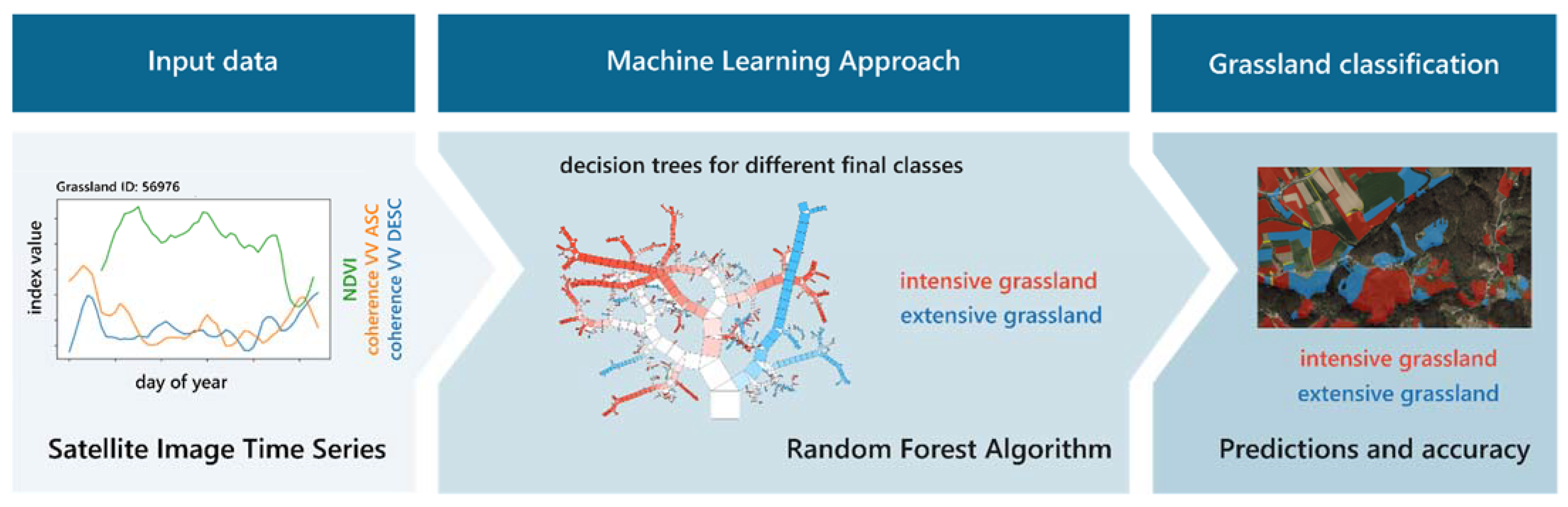
  • To analyse and evaluate the potential of intra-annual (from 2017 to 2019) Sentinel-1/2 SITS for distinguishing between intensively and extensively managed grassland at the parcel level.
  • To identify the importance of input features (acquisition dates, environmental variables, etc.) for grassland use intensity classification accuracy with Random Forest algorithm and combined multisensor SITS.

2. Materials and Methods
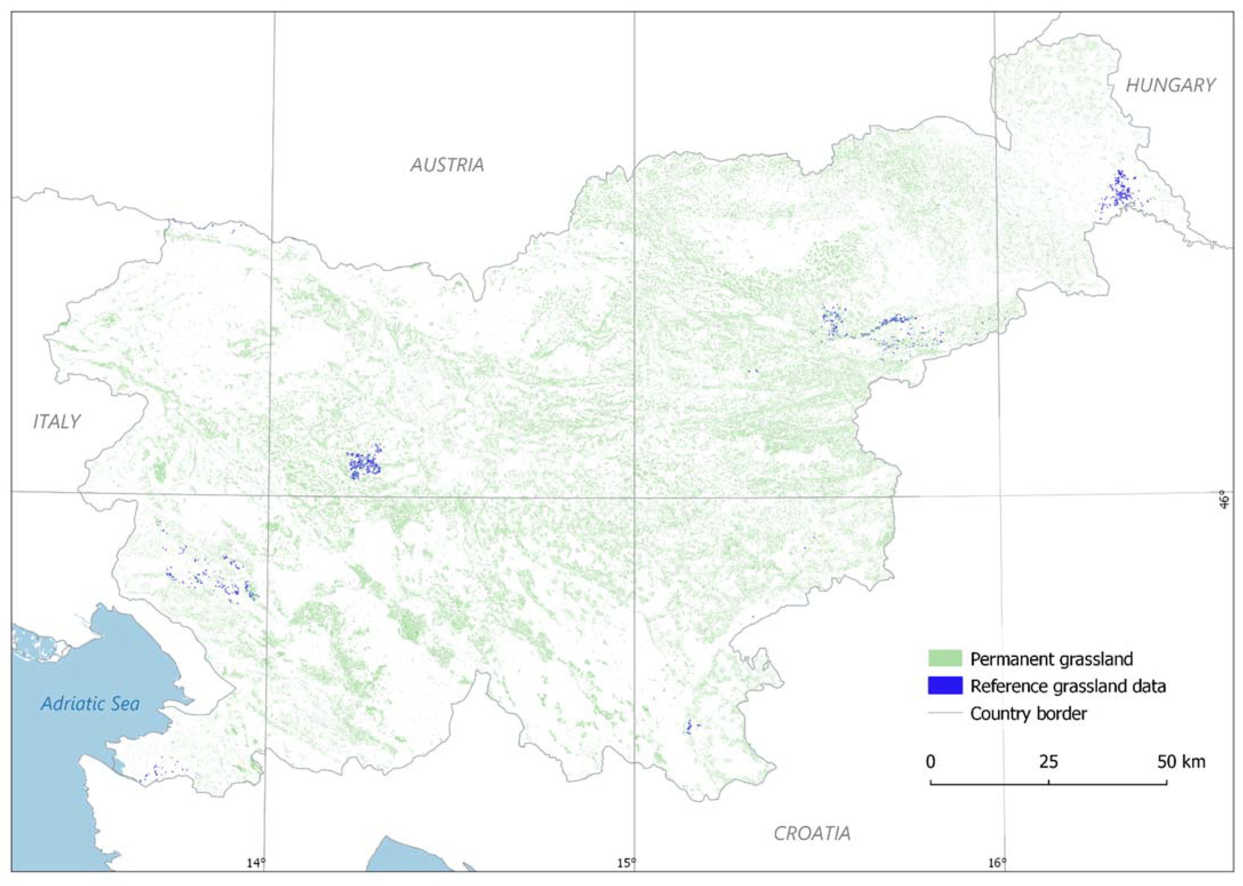
The methodological workflow consists of the following steps: (1) pre-processing and analysis of multisensor SITS; (2) object-orientated Random Forest classification and feature importance assessment; and (3) classification accuracy assessment. The sequence and linkage of steps are shown in the workflow presented in Figure 1.
We generated and analysed multivariate time series in the open-source Python library eo-learn [23,24]. For the classification task, we used the free software CLUS (ver. 2.12) [25]. CLUS is a decision tree and rule induction system that implements the predictive clustering framework. This framework combines unsupervised clustering and predictive modeling and allows an extension to more complex prediction settings such as multi-task learning and multi-label classification [25]. The feature importance evaluation and accuracy assessment were created in a free statistical software R (ver. 4.0.2) [26].

2.1. Study Area

The study area is permanent grassland throughout Slovenia (Figure 2). Slovenia is located in Central Europe, combining four major geographical units—the high Alps with their pre-Alpine hills, the rugged Dinaric Alps, the flat land of the Pannonian Plain with its hilly edge, and the Mediterranean hills with the moderating effect of the Adriatic Sea [27]. The area of permanent grassland is defined by the official MKGP (Ministry of Agriculture, Forestry and Food) land use layer RABA (record of agricultural and forest land use). The permanent grassland mask used in the study covered 305,884 ha, more than 15% of the total land area. The study area is heterogeneous in climate, soil, elevation, aspect and slope. The grasslands range from 10 m to 1600 m a.s.l., with a mean polygon area of 0.5 ha, an elevation of 430 m a.s.l., a slope of 8.6° and an aspect of 175.6°.

2.2. Reference Grassland Data and Training Dataset

Grassland is very diverse and heterogeneous. This seems to be an obstacle for analyses based on remote sensing data [18]. The reference data for grassland intensity use classification in Slovenia are represented by the field mapping of habitat types (2010–2020) carried out by the Institute of the Republic of Slovenia for Nature Conservation [28]. The basis for the fieldwork is the detailed classification of Slovenian habitat types [29] and the aerial orthophotos on which the boundaries of individual habitat types are mapped. The information on habitat types is based on the Palaearctic classification (PHYSIS database). The PHYSIS system of habitat classification was initially developed as part of the CORINE programme of the European Union for the selection and description of sites of nature conservation importance [30]. We worked on examples of semi-natural grassland, mesophilic meadows and secondary grassland. Natural and semi-natural grassland represented extensive samples with high biodiversity value, while secondary grassland and mesophilic meadows represented intensive samples with highly intensively managed grassland (Table 1).
First, we have reclassified the detailed habitat typology to the more general land cover, i.e., intensive and extensive grassland classes. We obtain an imbalance dataset of 9943 extensive and 1846 intensive grassland samples. The success of supervised classification, such as Random Forest, depends on the quality of the training dataset and the ability of the classifier to learn from the training dataset. With extremely imbalanced data, one cannot achieve good accuracy. Therefore, we manually prepared a new balanced reference dataset, a subset of the existing reference dataset with high-quality ground truth data.
We performed quality control on the prepared grassland dataset by visually evaluating the existing land cover information (checking whether it is grassland or something else) by reviewing the latest national orthophotos and Google Earth images. Finally, for the classification of grassland land use intensity, the training dataset contains 491 extensive and 768 intensive grassland polygons (blue features in Figure 2).

2.3. Sentinel-1/2 Images Pre-Processing

For grassland intensity classification, we use the time series analysis (TSA) approach based on all available Sentinel-1 and Sentinel-2 satellite scenes acquired between 1 March 2017 and 30 November 2019. For the multispectral Sentinel-2A and -2B data, we use the fully automated image processing chain STORM [31], which performs downloading the data from the Copernicus Open Access Hub, pre-processing the data (geometric, atmospheric and topographic corrections), cloud detection, and creating a mosaic from images acquired in the same orbit. We used all Sentinel-2 images covering Slovenia—in total 586 S2 images (approx. 190 per year), which means 1.82 TB storage. The TSA approach uses the four spectral bands with the spatial resolution of 10 m, i.e., the bands B02 (blue), B03 (green), B04 (red), and B08 (near-infrared). Because band ratios are less affected by atmospheric and topographic effects than single band values, we chose three spectral indices suggested for vegetation analysis in literature [32], i.e., NDVI, Enhanced Vegetation Index (EVI) and Modified Soil Adjusted Vegetation Index (MSAVI). We found that all three indices are highly correlated on permanent grassland in Slovenia and used only NDVI in the further analysis.
Sentinel-1 data in Interferometric Wide (IW) swath mode, providing dual polarisation data (VV + VH), were used in the analysis. A custom processing chain, based in part on the SNAP tool supplied by European Space Agency with additional steps to calculate sigma0 and coherence products every six days, was developed [33]. We used 2521 S1 images (approx. 840 per year), which means 11.6 TB of local storage.
For this study, we used only coherence, the estimate of the complex correlation coefficient. Given two complex SAR images s1 and s2 (e.g., Sentinel-1 Single Look Complex SLC products), coherence is defined as
γ = | s 1 s 2 * | s 1 s 1 * s 2 s 2 * ,   0 γ 1
where | . . | denotes the absolute value, . . an averaging operation, and ∗ the complex conjugate product [16].
The coherence reaches the maximum value when the position and physical properties of the scatters within the averaging window . . are the same for both s1 and s2. Changes in scatter distribution or placement, on the other hand, lead to a decrease in coherence. Temporal decorrelation in the coherence time series shows changes in the radar images over time. The growth of vegetation decreases correlation, while removing the grassland increases the correlation, leading to increased coherence [16]. Coherence can therefore be used to distinguish between intensive and extensive grassland management, as intensive grassland is mowed more frequently in a year than extensive grassland.

2.4. Environmental Variables

Because of the very large-scale and heterogeneous study area, we included extended set of topographic data in the model. Elevation, slope and aspect were derived from DEM with a resolution of 25 m, provided by the Surveying and Mapping Authority of the Republic of Slovenia (GURS). Elevation was measured in meters above sea level, slope and aspect in degrees. Elevation, aspect and slope have an indirect influence on plant growth and development due to temperature and solar radiation differences and runoff [15].

2.5. Mapping Units of Grassland Areas

2.5.1. Permanent Grassland Polygons

The conservation of permanent grassland is one of the objectives of the EU Common Agricultural Policy (CAP), which contributes to the overall climate and biodiversity objectives of the EU [34]. Each EU member state has its own nomenclature for classifying grassland polygons, recorded in Land Parcel Identification System (LPIS) to implement the CAP of the EU. LPIS in Slovenia is a part of the farm register and functions as a spatial representation of land used by agricultural holdings. The reference parcel of LPIS is the farmer block, a compact area of agricultural land used by a farm. Graphic units of agricultural parcels (GERK) are compact areas of agricultural land with the same type of land use within each block [35]. LPIS data for all GERK in Slovenia are freely available [36]. Permanent grassland, together with permanent pasture, is a land use on which grasses or other herbaceous forage grow naturally (self-seeded) or by cultivation (sown) and which has not been included in the crop rotation of a holding for at least five years [37]. However, not all permanent grassland polygons are included in the GERK database. For the grassland area, which is part of permanent grassland but not included in GERK, we created new objects by image segmentation.

2.5.2. Permanent Grassland Segments

Image segmentation was performed in the Harris ENVI Feature Extraction (ver. 5.3) software using the Sentinel-2 mosaic with the acquisition date of 30 June 2019 for the entire Slovenia. Only bands with 10 m resolution were used as colour space input (i.e., bands 2-4, 8) and hue, saturation, and intensity as band ratio attributes. We masked the mosaic with permanent grassland layer RABA and applied the integrated edge-based Full Lambda-Schedule algorithm [38] to extract features of the grassland-masked mosaic. The best segmentation result was obtained by setting the parameter Scale Level to 20 and Merge Level to 70, with a 7 × 7 low pass filter, to effectively delineate features at a similar spatial level as is the case with permanent grassland polygons in the GERK database. Segments smaller than 10 pixels were eliminated. The segmentation layer was then merged with GERK to form a common dataset of 519,611 mapping units (polygons) for classification.

2.6. Preparing Time Series with Eo-Learn

We created the processing pipeline using the open-source Python library eo-learn [23,24]. Due to the large amount of Sentinel-1 and -2 images (Section 2.3), we first divided the AOI into smaller patches of rectangular bounding boxes with dimensions 10 × 10 km, which can also be processed in case of limited computational resources. Then we started constructing the dense coherence SITS by stacking the Sentinel-1 coherence product and NDVI SITS by stacking the Sentinel-2 images and cloud masks into EOPatches. The result is a multidimensional NumPy array with information on raster width, height, the date of image acquisition, and the values of all bands. We removed the unusable pixels by applying the cloud masks (i.e., pixels with clouds, shadows, snow, haze) from the temporally stacked images. Due to the non-uniform acquisition dates of the satellite images provided by the different orbits covering Slovenia and missing values (especially for optical Sentinel-2 images), we applied a five-day linear interpolation to fill the missing gaps in SITS and create a common interval for all data.
Once bands and multi-image features are stored in EOPatches with uniform dates, they must be prepared for classification [28]. Supervised classification methods, such as Random Forest, require a labeled and unlabeled raster or vector dataset. For the labeled dataset, we used polygons with information about the intensity of grassland use (Section 2.2). For classification, we used permanent grassland polygons (Section 2.5). Both datasets were in a shapefile format. Subsequently, the polygons were buffered 7 m inwards to avoid edge effects and consider only interior pixels. The inter-annual SITS was generated for all polygons. The constructed SITS was based on the 75th percentile of the index value (NDVI, coherence VV ascending, and coherence VV descending) calculated on the pixels within the polygon and time stacked. The NDVI SITS was also masked with a threshold of 0.25, as we found that lower values did not represent grassland use. The SITS vectors were smoothed using Savitzky–Golay filter [39]. We used a window size of 21 pixels and a first-degree polynomial for filtering coherence SITS. For NDVI, we use a moving average window with the dimension corresponding to 20% of the interval in SITS and a second-degree polynomial.

2.7. Random Forest Classification Approach and Feature Ranking

Random Forest (RF) is an ensemble classifier that consists of a combination of decision trees [40]. The construction of the decision tree starts at the root, where it is calculated which input feature partitions the samples in a way that reduces the variance of the remaining samples. This results in two nodes that repeat the procedure and further reduce the variance of the remaining samples. This produces the desired number of decision trees forming an RF that votes on the most likely class for the samples. The classes, in our case, are intensively managed grassland and extensively managed grassland. Input features are time values of NDVI and coherence SITS (Section 2.6) with auxiliary environmental variables (Section 2.4).
Feature ranking is an essential task in machine-learning approaches. With ranking scores, we can reduce the high-dimensionality of the input dataset such that only the features that are the most informative about the target classes are kept. By using a scoring function, we estimate the importance ( x i ) values of the descriptive attributes (features) x i and rank the features based on their estimated importance [41]. In this study, we evaluate the importance of x i by measuring the Mean Decrease Accuracy (MDA), also known as the permutation importance [42]. The MDA measure has been widely used similarly in other classification studies [17,43,44,45]. MDA quantifies the importance of a feature by measuring the change in prediction accuracy when the values of the feature are randomly permuted compared to the original observations [46]. The importance of the feature is determined by comparing the resulting misclassification rate to the rate obtained without randomly permuting the values of the feature. This procedure is repeated for each feature [40]. We used MDA for a stepwise recursive feature selection approach similar to other studies [47,48].

3. Results

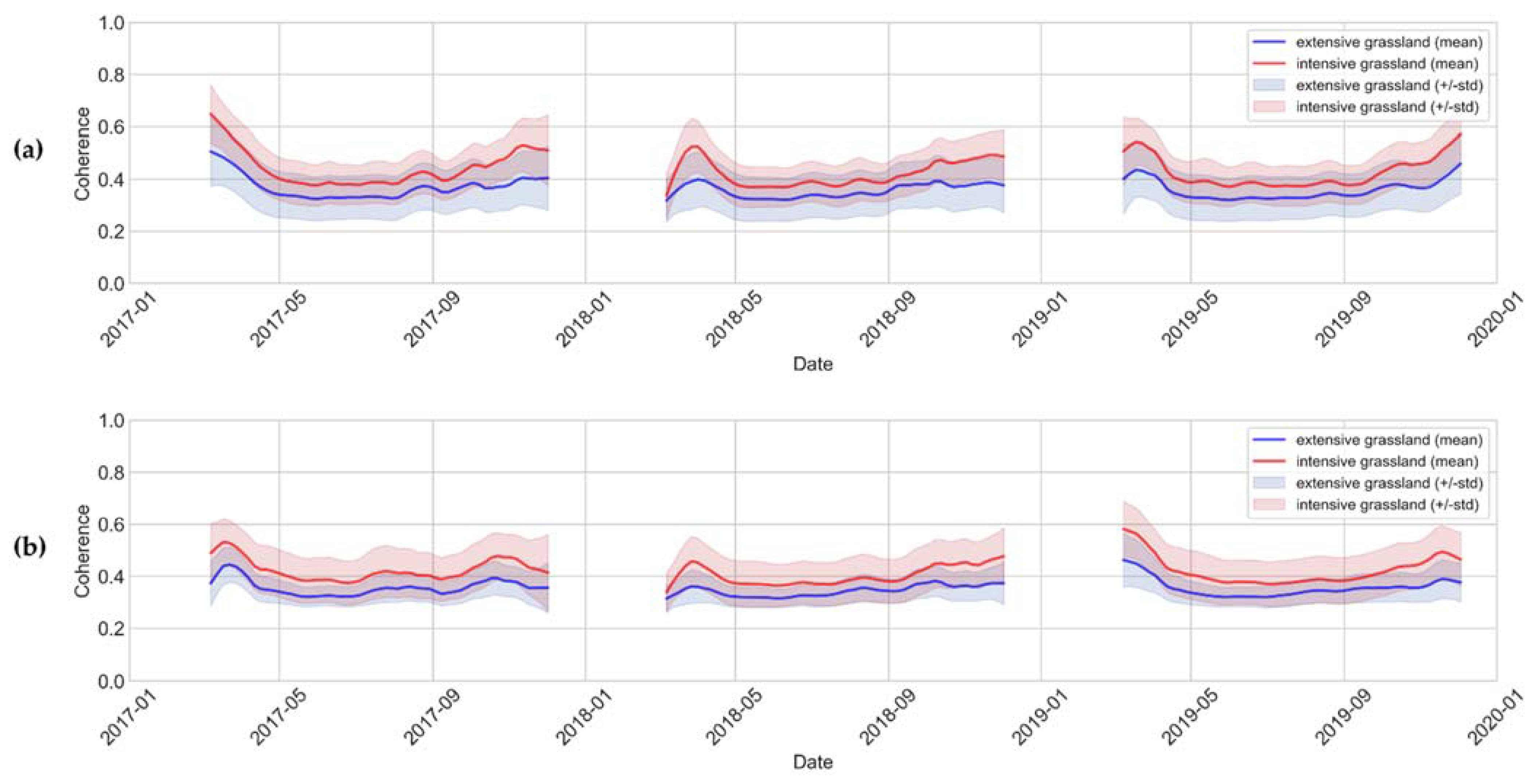
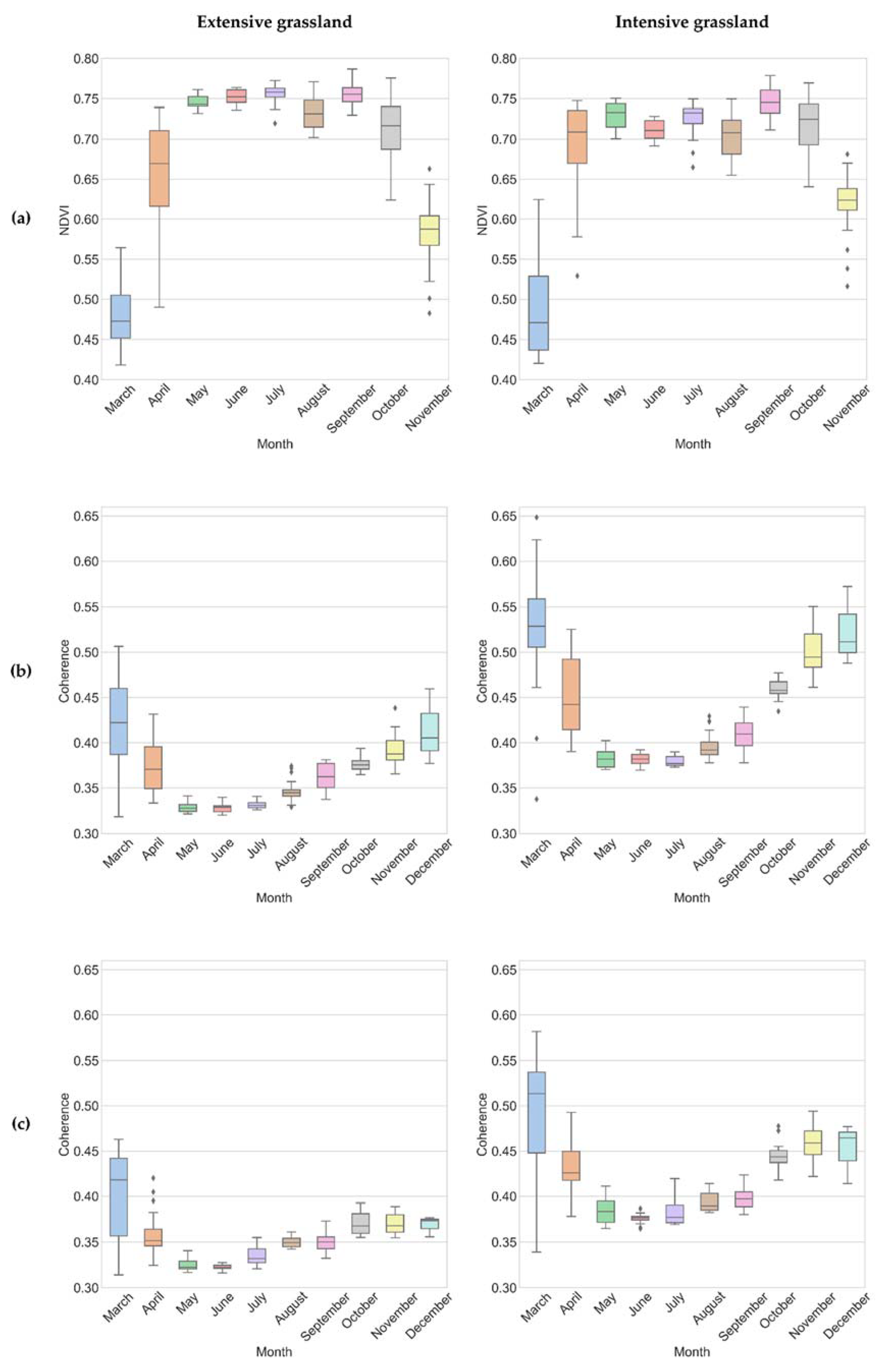
3.1. NDVI and Coherence SITS Analysis

For an assessment of class separability, annual NDVI, coherence VV ascending and coherence VV descending SITS were analysed class-wise based on the reference dataset of the 491 extensive and 768 intensive training samples. We examined the difference between Sentinel-1 and Sentinel-2 data for permanent grassland types in Slovenia. Finally, we analysed 519,611 grassland polygons, where 56% of the samples (283,256 polygons) were classified in the same intensive or extensive grassland class in all years studied. This database formed the basis for further TSA results.
NDVI values are related to the chlorophyll content of vegetation and depend on the grassland type and management practices [8]. Temporal profiles of NDVI values give an overview of the dynamic phenological processes of a particular grassland type and help identify specific events, such as mowing dates, etc. [18,21]. The mean temporal profiles and the standard deviation range of NDVI values (Figure 3) show the main difference between intensively and extensively managed grassland in Slovenia. Due to unpredictable gaps in the Sentinel-2 SITS, caused by unfavourable weather conditions, there were some differences in the results between the years studied. However, grass growth generally starts in March, accelerates in April, reaches its first maximum in May, and lasts in September. The drops in the NDVI values can be related to the mowing dates. We found that the first maximum is reached earlier in intensively managed grassland than in extensive grassland, while the last maximum is reached at the same time (at the end of September) in both grassland types. This confirms that intensively managed grassland is on average mowed significantly earlier (early May) than extensively managed grassland.
The mean temporal profiles of NDVI values for the studied grassland types differ significantly at the beginning of the growing season (in April) when NDVI values are lower on extensive grassland than on intensive grassland. However, extensively managed grassland generally reaches higher NDVI values during the season than intensively managed grassland. Therefore, the distribution range of mean NDVI values is different for intensive and extensive grassland. Annual NDVI values on extensive grassland range from 0.63 to 0.75 (median NDVI ≈ 0.74) and on intensive grassland from 0.66 to 0.74 (median NDVI ≈ 0.71).
The Sentinel-1 coherence VV (vertical transmit, vertical receive) polarised temporal profiles are analysed separately for ascending and descending orbits. The coherence time series profiles illustrated how the physical state of grasslands is represented in SITS. We can detect the presence of low/high vegetation or bare soil or see the growth and loss (mowing events) of vegetation [49]. Figure 4 shows the mean coherence time series profiles for each analysed class, Figure 4a for ascending orbit and Figure 4b for descending orbit.
High values of coherence represent low/no vegetation and a stable state. Low values of coherence represent vegetation in a dynamic state. When the values increase, the condition of the recognised grassland has changed. Statistical analysis showed that changes, such as cutting and plowing, cause an increase in coherence compared to the values before an event [50]. The result indicates that annual mean coherence values were statistically significantly higher on intensively managed grassland than on extensively managed grassland. The time series profile is smoother because there are more polygons in different parts of the studied country, where there are also differences in management practices at the time of change events. The difference in median values in the coherence time series for intensive and extensive grassland was significant in all analysed years (i.e., 2017 to 2019).

Relationship between NDVI and Coherence

Figure 5 shows the relationship between three-year monthly average NDVI and coherence time series data for extensive and intensive grassland types. There is no strong correlation because coherence and NDVI illustrate different grassland parameters. NDVI is mainly sensitive to the green, chlorophyll-containing biomass, whereas coherence is a normalised measure of change between two complex radar images [50] and is more sensitive to vegetation physical variations. Nevertheless, the NDVI and coherence SITS trend is clear—high NDVI corresponds to low coherence, and vice versa.

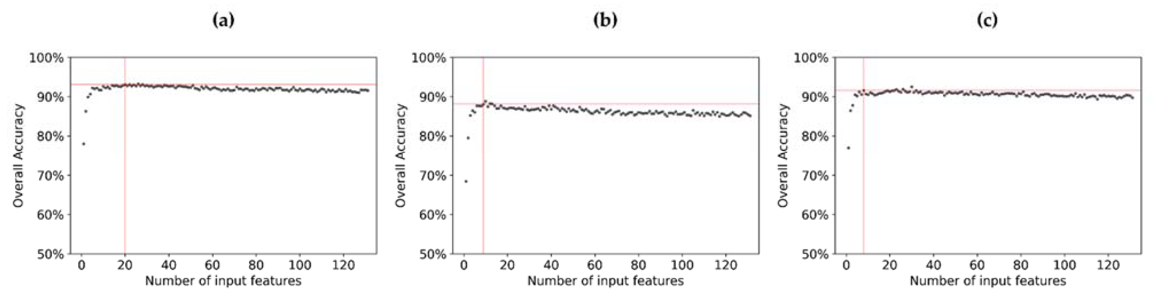
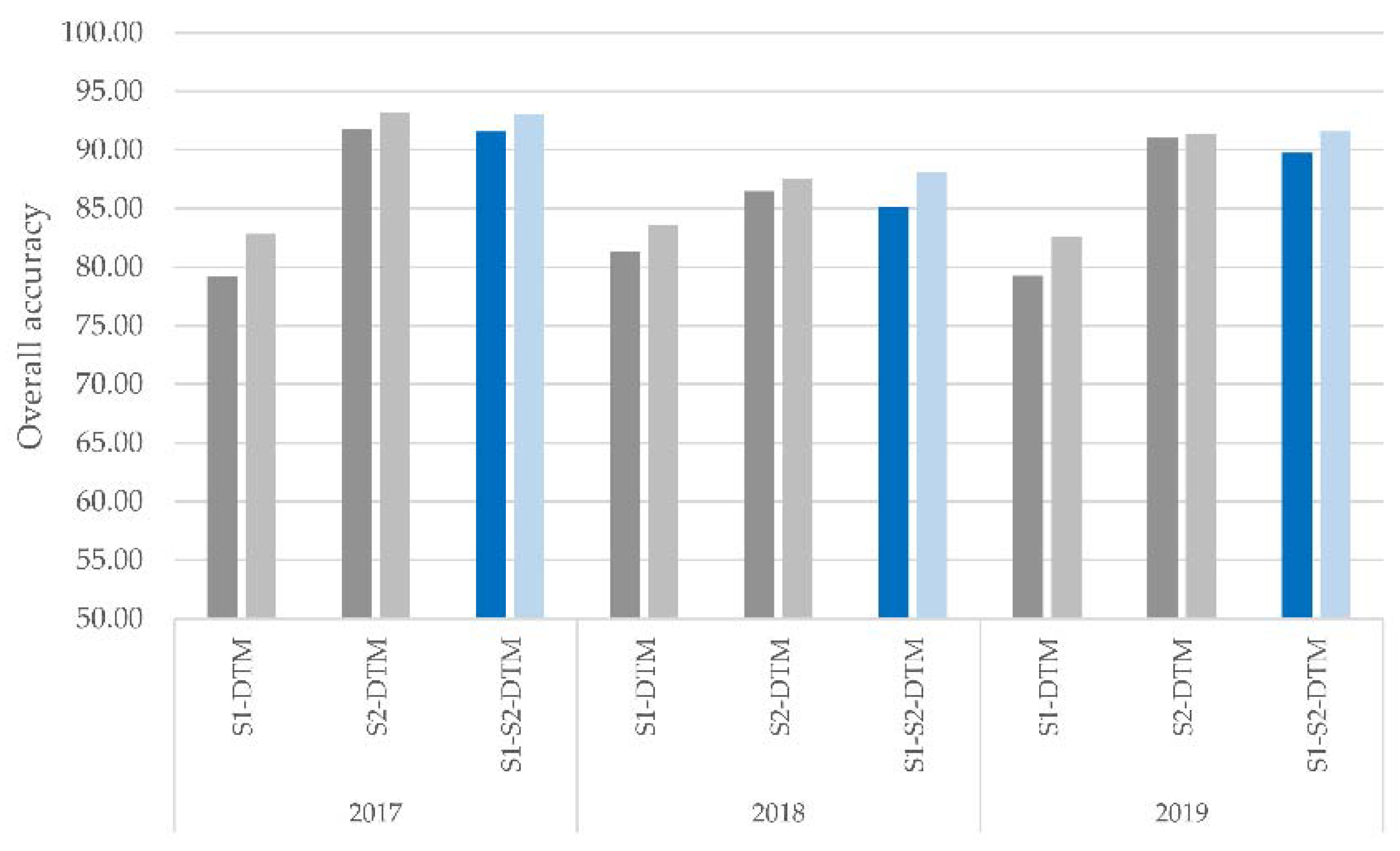
3.2. Grassland Classification Accuracy and Feature Selection

The classification was performed at the local level for each grassland polygon (total of 519,611 mapping units) of 30,588 ha of permanent grassland in Slovenia. The model was trained on the same reference dataset of intensive and extensive grassland polygons. Input model data were combined annual SITS (about 130 different Sentinel-1 and Sentinel-2 images each year) of two different remote sensing attributes—NDVI and coherence (separately ascending and descending orbit). Additionally, we experimented with three environmental variables (slope, aspect and elevation). Satellite images in the annual SITS are acquired between March and December. Results in the confusion matrices are calculated using 10-fold cross-validation on the reference dataset for the object-based classification of grassland use intensity type.
In Table 2, we summarise the results based on SITS only. In 2017 and 2019, the models achieved 84% and 80% OA, respectively. In 2018, the OA was 70%, which could be related to having the fewest cloud-free observations. Even with radar data, there is not enough information to distinguish between the two classes.
Because we know the location of the polygons, we can also calculate environmental variables such as elevation, slope, and aspect (from the digital terrain model DTM). With this information alone, we can distinguish the two grassland types quite well, with an overall accuracy of 79% (Table 3). In areas with lower elevations and slopes, intensive grassland is quite common. However, the results are not as good as when we have enough cloud-free observations.
In the following experiments, we combined environmental variables with the SITS to first evaluate the contribution of individual SITS. The results presented in Figure 6. show significant differences in the overall accuracies (OAs) between the RF model, where we used annual NDVI inputs (S2) or coherence (S1). The lowest overall classification accuracy was obtained when only radar coherence was combined with environmental variables (S1-DTM). The NDVI, in combination with environmental variables (S2-DTM) gives better results. We obtain the highest OA in all analysed years with combined optical and radar time series (S1-S2-DTM). The overall accuracy ranges from 85% to 92%. We optimised the results using MDA feature selection and achieved the best performance (OA ranging from 88% to 95%).
Figure 7 shows the number of features and the achieved OA using the RF algorithm over the years analysed. All available features were not equally important for grassland intensity classification. Using MDA, we were able to select only the essential features for a given year and improved the final classification accuracy by 2–3 percentage points. For example, there were a larger number of important features in 2017 (20) than in 2018 (9) and 2019 (8). The most important features for each year in the study area are listed in Table 4.
Slope, elevation and NDVI values at the beginning of the growing season (from April to June) proved to be the most important features to distinguish between intensive and extensive grassland in the analysed period. In 2017 and 2018, some radar coherence data were also included as an important feature. This proves the suitability of combining NDVI and coherence to identify the management intensity of grassland use.
Table 5 (combined annual SITS) and Table 6 (combined annual SITS using best feature selection) show substantial differences between annual accuracies. Grassland classification evaluation depends on the quality and availability of satellite imagery in the annual SITS. The RF algorithm achieved better classification results in 2017 and 2019, while the lowest accuracies and kappa coefficients were obtained in 2018. The producer’s and user’s accuracy of grassland types also varied from year to year. Intensive grassland provided more stable results in terms of accuracy (UA varied between 93% and 95%) than extensive grassland, where UA ranged between 73% and 90%, during the period studied.
The results for 2018 differ from the results of the other years, especially for extensive grassland; where the model gets the highest misclassification rate, user accuracy is only 73% (Table 5) and 81% in the case of using only the most relevant features based on MDA values (Table 6). The difference in the 2018 results can also be seen in the time series profiles in Figure 3 and Figure 4. The beginning of the growing season is clearly different from the other years analysed, where missing data (observation gaps) accumulated in Sentinel-2 SITS due to unfavourable weather in April and May.
Compared to Table 6, OA improved between 7–15%, most significantly in 2018. As before, there was still not enough information available from the SITS alone. This trend can also be seen in the UA for all years except the intensive grasslands of 2018, while the PA has increased in all comparisons.
We produced the final maps of permanent grassland use intensity based on the classification accuracy assessment. For each year, we produced a map of intensive and extensive grassland types for the entire country. Figure 8 illustrates the results of the object-based classification approach for three representative subsets of the study area. We can also obtain the confidence interval value associated with the prediction using the RF algorithm. The interval ranges from 0 to 10, where 0 represents extensive grassland use, and 10 represents intensive grassland use. Figure 8c shows that it is generally difficult to clearly determine the degree of intensity of grassland use. This is also the reason why there is still no clear definition of grassland use type, use intensity and grassland condition [18].

4. Discussion

This study has shown that multisensor time series of combined optical and radar remote-sensing data combined with environmental variables can effectively classify intensive and extensive grasslands in a large area of heterogeneous grassland stands. Several studies have highlighted the potential of Sentinel-1 and -2 data to characterise and classify different land use types, either separately or combined [15,51]. Still, only a few have used multisensor remote sensing imagery for grassland management and intensity use classification [8,18]. Most studies examined relatively small study areas with homogeneous intensity levels among grassland plots; however, larger heterogeneous landscapes with different environmental conditions and practices pose a challenge. Nevertheless, combined Sentinel-1 and -2 imagery to identify and characterise detailed grassland use remains underexplored. In this context, we seek to assess the potential of separate and combined Sentinel-1 and Sentinel-2 SITS for identifying and classifying the intensity of grassland use in a large study area covering the entire Slovenia. Our research analysed the RF algorithm in the combination of two different remote sensing products, optical NDVI and radar coherence, separately for the ascending and descending orbits, to identify the most appropriate features for grassland intensity use or management type separation.
Reinermann et al. [18] noted that in most studies on remote sensing of grassland, optical satellite data were used as vegetation indices, with NDVI representing grassland conditions well. Several studies have investigated radar-based backscatter amplitudes, interferometric coherence, and polarimetry-based decomposition parameters, primarily for grassland mowing detection rather than general type classification [50,52,53,54]. In the present study, the combination of NDVI and coherence proved to be very useful and robust for grassland classification at a larger spatial scale.
In addition to the final grassland classification, our study improved understanding of the relationships between the separate and combined multisensory SITS of NDVI and coherence and the estimated biophysical parameters, such as individual grassland characteristics related to management or intensity use. Temporal analysis of satellite-based information allows us to gain insight into the dynamic phenological processes of a particular grassland type and specific events, such as mowing, etc. [18,21,22,55,56].
Our study demonstrates the value of combining NDVI and coherence SITS for mapping and monitoring grassland use. Both SAR coherence and NDVI provided useful information for distinguishing between intensively and extensively managed grassland types. Temporal coherence profiles showed lower values for extensive grassland than for intensive grassland, while the opposite was observed for optical NDVI. Comparing optical Landsat and radar data ERS-2 SAR, Price et al. [57] found that NDVI values were more important than radar backscatter data for classifying grassland types. Bekkema et al. [8] concluded that for accurate grassland classification using only optical remote sensing data, the availability of satellite imagery in spring, preferably taken in April before the first mowing date, is essential. Our study showed similar results. NDVI values at the beginning of the growing season (in April and May) were the most important variables for separating intensive and extensive grassland. They can identify the main phase of highly dynamic vegetation growth [8]. Radar coherence improves classification accuracy when the number of cloud-free optical images is insufficient in a given season. Coherence SITS are particularly useful in areas with high cloud cover, such as the Alps and pre-Alps areas.
However, there were no direct correlations between NDVI and coherence because NDVI indicates biophysical grassland variables, whereas coherence captures more vegetation physical variation and change. Nevertheless, coherence SITS behave inversely to NDVI SITS (Figure 5). It reaches high values in the early and late seasons and low in the middle [50], indicating the possibility and new opportunity to improve the time series classification approach to create denser fused radar-optical SITS. Research, including ours, suggests that radar coherence SITS is better suited for detecting specific events at the level of individual plots, such as mowing and grazing dates, and then incorporating these parameters into more advanced classification analysis. Therefore, NDVI and coherence time series are beneficial for grassland mowing detection [10,50,58,59] and can further improve grassland intensity mapping capabilities.
Many studies have used the RF algorithm for grassland management or intensity classification [7,18,60]. Grabska et al. [61] found that topographic variables can improve the accuracy of vegetation classification of RF in large heterogeneous areas because they have an indirect influence on plant growth [15]. In our study, slope and elevation were also classified as features with a higher importance in all analysed years.
Using MDA, we reduced the dimensionality of the input SITS and found out which satellite image acquisition dates and attributes are more important/informative to build a model to discriminate between intensively and extensively managed grassland in a given year. In addition, the MDA criterion provided as an output of the RF classifier proved to be very efficient for feature selection. The overall accuracy (RF, object-based classification) obtained with the combination of all available annual features determined by MDA was only 2–3% lower than that obtained with the best feature selection combination (Figure 7).
Classification accuracy was assessed using OA, PA, and the Kappa coefficient. Extensive grassland had a significantly lower producer and user accuracy than intensive grassland in all years studied, regardless of the combination of input data. For example, in 2017, user accuracy was 91% (RF, object-based, 2 classes, 20 selected features), while for intensive grassland it was 95%. In 2018, user accuracy for extensive grassland was only 81% (RF, object-based, 2 classes, 9 selected features), while for intensive grassland it was 93%. In 2019, the user’s accuracy for extensive grassland was again higher, at 87% (RF, object-based, 2 classes, 8 selected features), while for intensive grassland it was 94%. The low accuracies for extensive grassland were obtained due to its high biodiversity value (depending on soil texture), the large study area with environmental diversity, and the unbalanced training dataset (39% polygons for extensive grassland and 61% polygons for intensive grassland). Therefore, further research is needed to determine how to expand and balance the number of reference training samples to improve grassland classification with additional attributes obtained from Sentinel SITS, including areas where samples are not currently representative.

5. Conclusions

This study aimed to improve the understanding of the combined dense multisensory Sentinel-1 and Sentinel-2 data SITS to classify two grassland types in a large and heterogeneous study area. We investigated the combination of two remote sensing products, optical NDVI and radar coherence, to classify grasslands. Including environmental variables in the classification further improved the classification accuracy of the results. We used the annual combined SITS for 2017, 2018, and 2019 and the RF algorithm to classify intensive and extensive grassland types. The analysis was carried out at the object (parcel) level. Using the MDA-based feature selection method, we reduced the number of model input variables by selecting the most relevant features (acquisition dates, environmental variables) to distinguish between intensive and extensive grassland types. This improved the final classification accuracy and provided deeper insights into large datasets of high-dimensional multisensory radar and optical SITS. The best classification accuracy was achieved with combined NDVI and coherence data. In particular, environmental variables and NDVI values at the beginning of the growing season, in April and May, showed high potential for effective classification of grassland use intensity. We also observed that radar was more important in the absence of NDVI data. Future work will focus on time series analysis to ensure robustness of the applied method, with the possibility of creating denser fused radar-optical SITS. An important next step is to gain deeper insights into the dynamic phenological processes of a given grassland type and specific events, such as mowing and grazing dates, and then incorporate these parameters into a more advanced classification approach to improve the final classification accuracy.

Author Contributions

Conceptualisation: A.P.B., T.V., M.R. and K.O.; methodology: A.P.B., T.V., M.R., K.O. and M.I.; validation: A.P.B., T.V., M.R. and M.I.; formal analysis: A.P.B.; investigation, A.P.B. and K.O.; resources: A.P.B. and T.V.; data curation: M.R. and M.I.; writing—original draft preparation: A.P.B.; writing—review and editing: K.O. and T.V.; visualisation: A.P.B.; supervision: K.O.; project administration: T.V.; funding acquisition: T.V. and K.O. All authors have read and agreed to the published version of the manuscript.

Funding

This research was funded by the Slovenian Research Agency research core funding Earth observation and geoinformatics (No. P2-0406), Anthropological and spatial studies (No. P6-0079) and research project M3Sat—Methodology of Multitemporal Multisensor Satellite Image Analysis (No. J2-9251), and LIFE integrated project for enhanced management of Natura 2000 in Slovenia (LIFE17 IPE/SI/000011).

Acknowledgments

We thank our project partner, the Institute of the Republic of Slovenia for Nature Conservation, for providing and helping with reference ground truth dataset and contextual discussion on analysis results.

Conflicts of Interest

The authors declare no conflict of interest.

References

  1. Lesschen, J.P.; Elbersen, B.; Hazeu, G.; van Doorn, A.; Mucher, S.; Velthof, G. Defining and Classifying Grasslands in Europe; Wageningen University and Research: Wageningen, The Netherlands, 2014. [Google Scholar]
  2. Wicke, B.; Kluts, I.; Lesschen, J.P. Bioenergy Potential and Greenhouse Gas Emissions from Intensifying European Temporary Grasslands. Land 2020, 9, 457. [Google Scholar] [CrossRef]
  3. Huyghe, C.; de Vliegher, A.; Gils, B.; Peeters, A. Grasslands and Herbivore Production in Europe and Effects of Common Policies; Editions Quae: Versailles, France, 2014; ISBN 978-2-7592-2157-8. [Google Scholar]
  4. Klein, N.; Theux, C.; Arlettaz, R.; Jacot, A.; Pradervand, J.-N. Modeling the effects of grassland management intensity on biodiversity. Ecol. Evol. 2020, 10, 13518–13529. [Google Scholar] [CrossRef] [PubMed]
  5. Nemecek, T.; Huguenin-Elie, O.; Dubois, D.; Gaillard, G.; Schaller, B.; Chervet, A. Life cycle assessment of Swiss farming systems: II. Extensive and intensive production. Agric. Syst. 2011, 104, 233–245. [Google Scholar] [CrossRef]
  6. Kuenzer, C.; Ottinger, M.; Wegmann, M.; Guo, H.; Wang, C.; Zhang, J.; Dech, S.; Wikelski, M. Earth observation satellite sensors for biodiversity monitoring: Potentials and bottlenecks. Int. J. Remote Sens. 2014, 35, 6599–6647. [Google Scholar] [CrossRef] [Green Version]
  7. Franke, J.; Keuck, V.; Siegert, F. Assessment of grassland use intensity by remote sensing to support conservation schemes. J. Nat. Conserv. 2012, 20, 125–134. [Google Scholar] [CrossRef]
  8. Bekkema, M.E.; Eleveld, M. Mapping Grassland Management Intensity Using Sentinel-2 Satellite Data. Giforum 2018, 1, 194–213. [Google Scholar] [CrossRef]
  9. Chiboub, O.; Kallel, A.; Frison, P.L.; Lopes, M. Monitoring of Grasslands Management Practices Using Interferometric Products Sentinel-1. In Advances in Remote Sensing and Geo Informatics Applications; CAJG 2018. Advances in Science, Technology & Innovation; El-Askary, H., Lee, S., Heggy, E., Pradhan, B., Eds.; Springer: Cham, Switzerland, 2019. [Google Scholar] [CrossRef]
  10. d’Andrimont, R.; Lemoine, G.; van der Velde, M. Targeted Grassland Monitoring at Parcel Level Using Sentinels, Street-Level Images and Field Observations. Remote Sens. 2018, 10, 1300. [Google Scholar] [CrossRef] [Green Version]
  11. Corbane, C.; Lang, S.; Pipkins, K.; Alleaume, S.; Deshayes, M.; García Millán, V.E.; Strasser, T.; Vanden Borre, J.; Toon, S.; Michael, F. Remote sensing for mapping natural habitats and their conservation status—New opportunities and challenges. Int. J. Appl. Earth Obs. Geoinf. 2015, 37, 7–16. [Google Scholar] [CrossRef]
  12. Ali, I.; Cawkwell, F.; Dwyer, E.; Barrett, B.; Green, S. Satellite remote sensing of grasslands: From observation to management. JPECOL 2016, 9, 649–671. [Google Scholar] [CrossRef] [Green Version]
  13. Nagendra, H. Using remote sensing to assess biodiversity. Int. J. Remote Sens. 2001, 22, 2377–2400. [Google Scholar] [CrossRef]
  14. Pettorelli, N.; Safi, K.; Turner, W. Satellite remote sensing, biodiversity research and conservation of the future. Philos. Trans. R. Soc. Lond. B Biol. Sci. 2014, 369, 20130190. [Google Scholar] [CrossRef] [PubMed]
  15. Holtgrave, A.-K.; Röder, N.; Ackermann, A.; Erasmi, S.; Kleinschmit, B. Comparing Sentinel-1 and -2 Data and Indices for Agricultural Land Use Monitoring. Remote Sens. 2020, 12, 2919. [Google Scholar] [CrossRef]
  16. Tamm, T.; Zalite, K.; Voormansik, K.; Talgre, L. Relating Sentinel-1 Interferometric Coherence to Mowing Events on Grasslands. Remote Sens. 2016, 8, 802. [Google Scholar] [CrossRef] [Green Version]
  17. Immitzer, M.; Neuwirth, M.; Böck, S.; Brenner, H.; Vuolo, F.; Atzberger, C. Optimal Input Features for Tree Species Classification in Central Europe Based on Multi-Temporal Sentinel-2 Data. Remote Sens. 2019, 11, 2599. [Google Scholar] [CrossRef] [Green Version]
  18. Reinermann, S.; Asam, S.; Kuenzer, C. Remote Sensing of Grassland Production and Management—A Review. Remote Sens. 2020, 12, 1949. [Google Scholar] [CrossRef]
  19. Niculescu, S.; Talab Ou Ali, H.; Billey, A. Random forest classification using Sentinel-1 and Sentinel-2 series for vegetation monitoring in the Pays de Brest (France). In Remote Sensing for Agriculture, Ecosystems, and Hydrology XX, Remote Sensing for Agriculture, Ecosystems, and Hydrology, Berlin, Germany, 10–13 September 2018; Neale, C.M., Maltese, A., Eds.; SPIE: Philadelphia, PA, USA, 2018; p. 6. ISBN 9781510621497. [Google Scholar]
  20. Meroni, M.; d’Andrimont, R.; Vrieling, A.; Fasbender, D.; Lemoine, G.; Rembold, F.; Seguini, L.; Verhegghen, A. Comparing land surface phenology of major European crops as derived from SAR and multispectral data of Sentinel-1 and -2. Remote Sens. Environ. 2021, 253, 112232. [Google Scholar] [CrossRef]
  21. Kolecka, N.; Ginzler, C.; Pazur, R.; Price, B.; Verburg, P. Regional Scale Mapping of Grassland Mowing Frequency with Sentinel-2 Time Series. Remote Sens. 2018, 10, 1221. [Google Scholar] [CrossRef] [Green Version]
  22. Mestre-Quereda, A.; Lopez-Sanchez, J.M.; Vicente-Guijalba, F.; Jacob, A.W.; Engdahl, M.E. Time-Series of Sentinel-1 Interferometric Coherence and Backscatter for Crop-Type Mapping. IEEE J. Sel. Top. Appl. Earth Obs. Remote Sens. 2020, 13, 4070–4084. [Google Scholar] [CrossRef]
  23. Lubej, M. Land Cover Classification with eo-learn: Part 1—Sentinel Hub Blog—Medium. Sentinel Hub Blog [Online]. Available online: https://medium.com/sentinel-hub/land-cover-classification-with-eo-learn-part-1-2471e8098195 (accessed on 12 May 2021).
  24. Lubej, M. Land Cover Classification with eo-learn: Part 2—Sentinel Hub Blog—Medium. Sentinel Hub Blog [Online]. Available online: https://medium.com/sentinel-hub/land-cover-classification-with-eo-learn-part-2-bd9aa86f8500 (accessed on 14 May 2021).
  25. Clus: A Predictive Clustering System. Available online: https://dtai.cs.kuleuven.be/clus/ (accessed on 16 May 2021).
  26. R: The R Project for Statistical Computing. Available online: https://www.r-project.org/ (accessed on 30 June 2021).
  27. Perko, D.; Ciglič, R. Slovenia as a European landscape hotspot. AGB 2015, 1, 45–54. [Google Scholar] [CrossRef]
  28. Zavod RS za Varstvo Narave. Kartiranje Habitatnih Tipov. Available online: https://zrsvn-varstvonarave.si/informacije-za-uporabnike/katalog-informacij-javnega-znacaja/habitatni-tipi/ (accessed on 24 June 2021).
  29. Jogan, N.; Kaligarič, M.; Seliškar, A. Habitatni Tipi Slovenije: Tipologija; Ministrstvo za okolje, prostor in energijo, Agencija RS za okolje: Ljubljana, Slovenia, 2004; ISBN 9616324209.
  30. PHYSIS A Classification of Palaeartic Habitats. Available online: http://cb.naturalsciences.be/databases/cb_db_physis_eng.htm (accessed on 24 June 2021).
  31. Oštir, K.; Čotar, K.; Marsetič, A.; Pehani, P.; Perše, M.; Zakšek, K.; Zaletelj, J.; Rodič, T. Automatic Near-Real-Time Image Processing Chain for Very High Resolution Optical Satellite Data. Int. Arch. Photogramm. Remote Sens. Spatial Inf. Sci. 2015, XL-7/W3, 669–676. [Google Scholar] [CrossRef] [Green Version]
  32. Tucker, C.J. Red and photographic infrared linear combinations for monitoring vegetation. Remote Sens. Environ. 1979, 8, 127–150. [Google Scholar] [CrossRef] [Green Version]
  33. Pehani, P.; Čož, N.; Veljanovski, T.; Kokalj, Ž.; Lisec, A.; Oštir, K. Automatic Processing of Sentinel-1 Sigma and Coherence: Technical Report; ZRC SAZU: Ljubljana, Slovenia, 2020. [Google Scholar]
  34. Viira, A.-H.; Ariva, J.; Kall, K.; Oper, L.; Jürgenson, E.; Maasikamäe, S.; Põldaru, R. Restricting the eligible maintenance practices of permanent grassland—A realistic way towards more active farming? Agron. Res. 2020, 18, 1556–1572. [Google Scholar] [CrossRef]
  35. Land Parcel Identification System (LPIS)—European Data Portal. Available online: https://www.europeandataportal.eu/data/datasets/8c8072f5-2075-49c3-b3e5-56ee58f8db8d?locale=en (accessed on 16 March 2021).
  36. MKGP—Portal. Available online: https://rkg.gov.si/vstop/ (accessed on 24 June 2021).
  37. European Court of Auditors. The Land Parcel Identification System: A Useful Tool to Determine the Eligibility of Agricultural Land—But its Management Could Be Further Improved; European Court of Auditors: Luxembourg, 2016.
  38. Robinson, D.J.; Redding, N.J.; Crisp, D.J. Implementation of a Fast Algorithm for Segmenting SAR Imagery; DSTO Electronics and Surveillance Research Laboratory: Edinburgh, Australia, 2002. [Google Scholar]
  39. Löw, M.; Koukal, T. Phenology Modelling and Forest Disturbance Mapping with Sentinel-2 Time Series in Austria. Remote Sens. 2020, 12, 4191. [Google Scholar] [CrossRef]
  40. Breiman, L. Random Forests. Mach. Learn. 2001, 45, 5–32. [Google Scholar] [CrossRef] [Green Version]
  41. Petković, M.; Kocev, D.; Džeroski, S. Feature ranking for multi-target regression. Mach. Learn. 2020, 109, 1179–1204. [Google Scholar] [CrossRef]
  42. Louppe, G. Understanding Random Forests: From Theory to Practice. Ph.D. Thesis, University of Liege, Liège, Belgique, 2014. [Google Scholar]
  43. Šandera, J.; Štych, P. Selecting Relevant Biological Variables Derived from Sentinel-2 Data for Mapping Changes from Grassland to Arable Land Using Random Forest Classifier. Land 2020, 9, 420. [Google Scholar] [CrossRef]
  44. Jin, Y.; Liu, X.; Chen, Y.; Liang, X. Land-cover mapping using Random Forest classification and incorporating NDVI time-series and texture: A case study of central Shandong. Int. J. Remote Sens. 2018, 39, 8703–8723. [Google Scholar] [CrossRef]
  45. Immitzer, M.; Atzberger, C.; Koukal, T. Tree Species Classification with Random Forest Using Very High Spatial Resolution 8-Band WorldView-2 Satellite Data. Remote Sens. 2012, 4, 2661–2693. [Google Scholar] [CrossRef] [Green Version]
  46. Calle, M.L.; Urrea, V. Letter to the editor: Stability of Random Forest importance measures. Brief. Bioinform. 2011, 12, 86–89. [Google Scholar] [CrossRef] [Green Version]
  47. Immitzer, M.; Böck, S.; Einzmann, K.; Vuolo, F.; Pinnel, N.; Wallner, A.; Atzberger, C. Fractional cover mapping of spruce and pine at 1 ha resolution combining very high and medium spatial resolution satellite imagery. Remote Sens. Environ. 2018, 204, 690–703. [Google Scholar] [CrossRef] [Green Version]
  48. Schultz, B.; Immitzer, M.; Formaggio, A.; Sanches, I.; Luiz, A.; Atzberger, C. Self-Guided Segmentation and Classification of Multi-Temporal Landsat 8 Images for Crop Type Mapping in Southeastern Brazil. Remote Sens. 2015, 7, 14482–14508. [Google Scholar] [CrossRef] [Green Version]
  49. Agricultural Practices | Sen4Cap. Available online: http://esa-sen4cap.org/content/agricultural-practices (accessed on 21 May 2021).
  50. Voormansik, K.; Zalite, K.; Sünter, I.; Tamm, T.; Koppel, K.; Verro, T.; Brauns, A.; Jakovels, D.; Praks, J. Separability of Mowing and Ploughing Events on Short Temporal Baseline Sentinel-1 Coherence Time Series. Remote Sens. 2020, 12, 3784. [Google Scholar] [CrossRef]
  51. Ienco, D.; Interdonato, R.; Gaetano, R.; Ho Tong Minh, D. Combining Sentinel-1 and Sentinel-2 Satellite Image Time Series for land cover mapping via a multi-source deep learning architecture. ISPRS J. Photogramm. Remote Sens. 2019, 158, 11–22. [Google Scholar] [CrossRef]
  52. Voormansik, K.; Jagdhuber, T.; Olesk, A.; Hajnsek, I.; Papathanassiou, K.P. Towards a detection of grassland cutting practices with dual polarimetric TerraSAR-X data. Int. J. Remote Sens. 2013, 34, 8081–8103. [Google Scholar] [CrossRef]
  53. Voormansik, K.; Jagdhuber, T.; Zalite, K.; Noorma, M.; Hajnsek, I. Observations of Cutting Practices in Agricultural Grasslands Using Polarimetric SAR. IEEE J. Sel. Top. Appl. Earth Obs. Remote Sens. 2016, 9, 1382–1396. [Google Scholar] [CrossRef]
  54. Taravat, A.; Wagner, M.; Oppelt, N. Automatic Grassland Cutting Status Detection in the Context of Spatiotemporal Sentinel-1 Imagery Analysis and Artificial Neural Networks. Remote Sens. 2019, 11, 711. [Google Scholar] [CrossRef] [Green Version]
  55. Stendardi, L.; Karlsen, S.; Niedrist, G.; Gerdol, R.; Zebisch, M.; Rossi, M.; Notarnicola, C. Exploiting Time Series of Sentinel-1 and Sentinel-2 Imagery to Detect Meadow Phenology in Mountain Regions. Remote Sens. 2019, 11, 542. [Google Scholar] [CrossRef] [Green Version]
  56. de Vroey, M.; Radoux, J.; Defourny, P. Grassland Mowing Detection Using Sentinel-1 Time Series: Potential and Limitations. Remote Sens. 2021, 13, 348. [Google Scholar] [CrossRef]
  57. Price, K.P.; Guo, X.; Stiles, J.M. Comparison of Landsat TM and ERS-2 SAR data for discriminating among grassland types and treatments in eastern Kansas. Comput. Electron. Agric. 2002, 37, 157–171. [Google Scholar] [CrossRef]
  58. Sen4Cap. Available online: http://esa-sen4cap.org/ (accessed on 21 June 2021).
  59. Gómez Giménez, M.; de Jong, R.; Della Peruta, R.; Keller, A.; Schaepman, M.E. Determination of grassland use intensity based on multi-temporal remote sensing data and ecological indicators. Remote Sens. Environ. 2017, 198, 126–139. [Google Scholar] [CrossRef]
  60. Asam, S.; Klein, D.; Dech, S. Estimation of grassland use intensities based on high spatial resolution LAI time series. Int. Arch. Photogramm. Remote Sens. Spatial Inf. Sci. 2015, XL-7/W3, 285–291. [Google Scholar] [CrossRef] [Green Version]
  61. Grabska, E.; Frantz, D.; Ostapowicz, K. Evaluation of machine learning algorithms for forest stand species mapping using Sentinel-2 imagery and environmental data in the Polish Carpathians. Remote Sens. Environ. 2020, 251, 112103. [Google Scholar] [CrossRef]
Figure 1. Methodological framework for time series object-based classification adopted in this study.
Remotesensing 14 03387 g001
Figure 2. Study area (entire Slovenia) with the permanent grassland cover and reference grassland data.
Remotesensing 14 03387 g002
Figure 3. The mean temporal profiles and standard deviation range (+/− std) of NDVI time series of intensive (red) and extensive (blue) grassland in Slovenia for the years 2017, 2018 and 2019.
Remotesensing 14 03387 g003
Figure 4. Mean temporal profiles and standard deviation range (+/− std) of coherence ascending (a) and coherence descending (b) time series on intensive (red) and extensive (blue) grassland.
Remotesensing 14 03387 g004
Figure 5. Boxplots of monthly average NDVI (a), coherence ascending (b) and coherence descending (c) for extensive and intensive managed grassland in all analysed years.
Remotesensing 14 03387 g005
Figure 6. Comparison of the overall accuracy of grassland Random Forest classification for all years analysed, using a different combination of input data—separate optical (S2), radar (S1), and combined (S1–S2) SITS with environmental variables used for grassland intensity classification. Darker colours show the overall accuracy achieved from all available features. Lighter colours show the overall classification accuracy achieved by the model approach with feature selection based on MDA values.
Remotesensing 14 03387 g006
Figure 7. Results of the Random Forest model for recursive feature selection to distinguish between intensive and extensive grassland classes, starting with the model based on all available features from combined optical and radar data and environmental data for 2017 (a), 2018 (b) and 2019 (c). The red lines show the selection of the final chosen model and the corresponding number of input features.
Remotesensing 14 03387 g007
Figure 8. Permanent grassland classification results for representative subsets of the study area. (a) Orthophoto, (b) intensive and extensive grassland use classification results for 2019 and (c) confidence interval value associated with the prediction. The representative subsets of the study area have different relief characteristics and management practices. Subset at the top is a mix of flat and rugged terrain, subset in the middle represents flat terrain, and subset at the bottom represents rugged Karst terrain.
Remotesensing 14 03387 g008
Table 1. Detailed habitat types and their subtypes were joined to represent general intensive and extensive grassland classes.
Grassland ClassPalaearctic Classification (PHYSIS Database)
extensive34.1, 34.2, 34.3, 34.7, 35, 36, 37.2, 37.3, 38.2
intensive38.1, 38.11, 38.13, 81, 81.1, 81.2
Table 2. Confusion matrices of the annual SITS (Sentinel-1, Sentinel-2) for the accuracy of the reference dataset with RF classifier (UA: User’s Accuracy, PA: Producer’s Accuracy, OA: Overall Accuracy). (a) is for the year 2017, (b) for 2018, and (c) is for 2019.
(a)Grassland classPredicted
2017ExtensiveIntensiveΣUA
Actualextensive3611304910.735
intensive667027680.914
Σ4278321259
PA0.8450.843OA0.844
Kappa0.665
(b)Grassland classPredicted
2018extensiveintensiveΣUA
Actualextensive1463454910.297
intensive327367680.958
Σ17810811259
PA0.8200.680OA0.700
Kappa0.289
(c)Grassland classPredicted
2019extensiveintensiveΣUA
Actualextensive3081834910.627
intensive627067680.919
Σ3708891259
PA0.8320.794OA0.805
Kappa0.572
Table 3. Confusion matrices of the environmental variables with RF classifier.
Grassland ClassPredicted
ExtensiveIntensiveΣUA
Actualextensive3161754910.644
intensive936757680.879
Σ4098501259
PA0.7730.794OA0.787
Kappa0.539
Table 4. RF model with the most important features for the analysed years. The last column indicates the value of the Mean Decrease in Accuracy (MDA).
YearThe Most Informative FeatureMDA
2017NDVI (2017-04-10)42.3
Slope40.5
NDVI (2017-04-30)25.3
NDVI (2017-04-05)24.5
NDVI (2017-04-15)25.8
NDVI (2017-05-05)24.3
Elevation22.7
NDVI (2017-05-10)22.5
NDVI (2017-05-20)20.9
NDVI (2017-05-25)19.8
NDVI (2017-04-20)20.3
NDVI (2017-05-15)19.1
coherence VV descending (2017-10-28)18.0
NDVI (2017-05-30)18.4
NDVI (2017-04-25)16.5
NDVI (2017-09-22)15.3
NDVI (2017-06-04)16.2
NDVI (2017-06-24)15.2
coherence VV ascending (2017-07-25)14.3
coherence VV descending (2017-05-06)16.0
2018Slope93.1
NDVI (2018-04-30)51.5
Elevation38.9
NDVI (2018-04-20)35.1
NDVI (2018-10-22)35.1
coherence VV descending (2018-09-18)30.2
coherence VV descending (2018-04-01)30.2
NDVI (2018-04-25)32.2
NDVI (2018-05-15)25.2
2019Slope55.9
NDVI (2019-04-10)45.8
NDVI (2019-04-20)39.0
NDVI (2019-04-15)29.3
Elevation32.2
NDVI (2019-06-19)29.7
NDVI (2019-06-09)30.9
NDVI (2019-05-10)25.6
Table 5. Confusion matrices of the annual SITS (all available Sentinel-1, Sentinel-2 and environmental variables) for the accuracy of the reference dataset with RF classifier (UA: User’s Accuracy, PA: Producer’s Accuracy, OA: Overall Accuracy). (a) is for the year 2017, (b) for the year 2018 and (c) is for the year 2019.
(a)Grassland ClassPredicted
2017ExtensiveIntensiveΣUA
Actualextensive437544910.890
intensive527167680.932
Σ4897701259
PA0.8940.930OA0.916
Kappa0.823
(b)Grassland classPredicted
2018extensiveintensiveΣUA
Actualextensive3591324910.731
intensive557137680.928
Σ4148451259
PA0.8670.844OA0.852
Kappa0.679
(c)Grassland classPredicted
2019extensiveintensiveΣUA
Actualextensive411804910.837
intensive497197680.936
Σ4607991259
PA0.8940.900OA0.898
Kappa0.782
Table 6. Confusion matrices of the annual SITS (using the best feature selection with MDA from Sentinel-1, Sentinel-2 and environmental data) for the accuracy of the reference dataset with RF classifier (UA: User’s Accuracy, PA: Producer’s Accuracy, OA: Overall Accuracy). (a) is for the year 2017, (b) for 2018 and (c) is for 2019.
(a)Grassland ClassPredicted
2017ExtensiveIntensiveΣUA
Actualextensive445464910.906
intensive417277680.947
Σ4867731259
PA0.9160.941OA0.931
Kappa0.855
(b)Grassland classPredicted
2018extensiveintensiveΣUA
Actualextensive395964910.805
intensive547147680.930
Σ4498101259
PA0.8800.882OA0.881
Kappa0.746
(c)Grassland classPredicted
2019extensiveintensiveΣUA
Actualextensive429624910.874
intensive447247680.943
Σ4737861259
PA0.9100.9211OA0.916
Kappa0.822
Publisher’s Note: MDPI stays neutral with regard to jurisdictional claims in published maps and institutional affiliations.

