Article

Crop Classification Based on GDSSM-CNN Using Multi-Temporal RADARSAT-2 SAR with Limited Labeled Data

1
School of Computer and Information Engineering, Henan University, Kaifeng 475004, China
2
Henan Engineering Research Center of Intelligent Technology and Application, Henan University, Kaifeng 475004, China
3
Henan Key Laboratory of Big Data Analysis and Processing, Henan University, Kaifeng 475004, China
4
Land Satellite Remote Sensing Application Center, Ministry of Natural Resources, Beijing 100048, China
*
Author to whom correspondence should be addressed.
Remote Sens. 2022, 14(16), 3889; https://doi.org/10.3390/rs14163889
Submission received: 7 July 2022 / Revised: 10 August 2022 / Accepted: 10 August 2022 / Published: 11 August 2022
(This article belongs to the Special Issue SAR-Based Signal Processing and Target Recognition)

Abstract

:
Crop classification is an important part of crop management and yield estimation. In recent years, neural networks have made great progress in synthetic aperture radar (SAR) crop classification. However, the insufficient number of labeled samples limits the classification performance of neural networks. In order to solve this problem, a new crop classification method combining geodesic distance spectral similarity measurement and a one-dimensional convolutional neural network (GDSSM-CNN) is proposed in this study. The method consisted of: (1) the geodesic distance spectral similarity method (GDSSM) for obtaining similarity and (2) the one-dimensional convolutional neural network model for crop classification. Thereinto, a large number of training data are extracted by GDSSM and the generalized volume scattering model which is based on radar vegetation index (GRVI), and then classified by 1D-CNN. In order to prove the effectiveness of the GDSSM-CNN method, the GDSSM method and 1D-CNN method are compared in the case of a limited sample. In terms of evaluation and verification of methods, the GDSSM-CNN method has the highest accuracy, with an accuracy rate of 91.2%, which is 19.94% and 23.91% higher than the GDSSM method and the 1D-CNN method, respectively. In general, the GDSSM-CNN method uses a small number of ground measurement samples, and it uses the rich polarity information in multi-temporal fully polarized SAR data to obtain a large number of training samples, which can quickly improve the accuracy of classification in a short time, which has more new inspiration for crop classification.

Graphical Abstract

1. Introduction

Crops are the basis for maintaining human civilization and are of great significance to human diet and social stability [1,2]. Obtaining crop planting distribution information is very important for growth monitoring, yield estimation and food security [3,4,5,6]. The ground survey is a traditional way to obtain information on crop planting distribution, which consumes a lot of time and money. Agricultural remote sensing technology, which offers the advantages of a large monitoring range and low cost, has gradually replaced the traditional methods [7,8].
Optical sensors have been widely used in crop classification for a long time [9,10,11]. However, optical sensors are limited by weather conditions. Images cannot be created in sufficient quality in the case of bad weather (such as cloudy, rainy or foggy) or during the nighttime [12,13]. Crops will experience significant changes to their shape at important phenological periods. However, many farmlands are obscured by clouds, making it more likely that the optical sensor will fail to capture images during the crucial phenological period for crops [14,15]. Synthetic aperture radar (SAR) is an active microwave sensor, which cannot be affected by cloudy and foggy weather [16]. Moreover, SAR is sensitive to the dielectric properties and structure of plants and is very suitable for monitoring and classifying crops [17,18]. In addition, polarimetric SAR (PolSAR), which can provide rich information, can extract a large number of polarimetric features. These polarimetric features are very valuable in crop classification [19,20]. Therefore, the multi-temporal RadarSat-2 image is used as the main data source of crop classification in this study.
There is a long history of extracting polarimetric features from PolSAR data for crop classification [21]. Polarization decomposition technology is the main method of extracting polarization characteristics [22,23,24] and has been used by researchers in agricultural remote sensing applications [25,26]. Guo et al. [26] used various features of H/α decomposition and support vector machine (SVM) to classify crops. The results show that the features obtained by polarization decomposition provide accurate polarization information, and the classification accuracy of crops exceeds 80%. The method of polarization decomposition is helpful for crop classification. However, the polarization decomposition method is sensitive to the target orientation and uses a specific volume model, which is rarely applicable to all phenological stages of different crops [27,28]. Therefore, there is great potential to classify crops by using polarization characteristics that correlate the relevant physical scattering mechanisms of vegetation canopy with phenology. It has been proved that the generalized volume scattering model which is based on the radar vegetation index (GRVI) can well reflect the relevant physical scattering mechanism of the crop canopy and follow the growth and development of crops [29,30].
Multi-temporal PolSAR has very rich characteristics [31]. In order to improve the accuracy of crop classification, people have proposed various methods to use the rich information in PolSAR, such as support vector machine [32] and random forest (RF) [33]. SVM and RF have attracted much attention because of their good performance and ease of use in limited training samples, but the feature extraction of these methods is still limited [34]. Because of the exceptional results in the area of computer vision, deep learning has become the mainstream method in the field of SAR image processing. In recent years, many scholars have proposed various deep learning methods for crop classification [35,36]. Zhang et al. [35] proposed a novel crop discrimination network with multi-scale features (MSCDN), which proved that the neural network can efficiently extract features in multi-temporal PolSAR, with an overall accuracy rate of crop classification of 99.33%. Chang et al. [36] proposed a convolutional long short-term memory rice field classifier (ConvLSTM-RFC) and demonstrated the effectiveness of the convolutional block attention module (CBAM) in handling multi-temporal features, with the highest accuracy of 98.08%. However, because sample sampling requires great time and money costs, the sample is often limited in the process of crop classification. These deep learning methods easily overfit and degrade the classification performance when the samples are limited [37,38,39]. Therefore, it is still a challenge to develop a multi-temporal PolSAR crop classification method in the case of limited samples.
The motivation of this study is to propose a multi-temporal and fully polarized crop classification method that can accurately classify crops with limited samples. Firstly, the geodesic distance spectral similarity measure (GDSSM) method is used to calculate the similarity between unlabeled pixels and the samples. Secondly, the open mask product Global Food Security-Support Analysis Data at 30 m (GFSAD) is used to generate a farmland mask in combination with GDSSM to extract farmland areas and non-farmland areas in the study area. Thirdly, multi-temporal backscattering coefficient and GRVI are extracted as features. Fourthly, the data with GDSSM greater than the threshold are selected as training data. Finally, the one-dimensional convolutional neural network (1D-CNN) is used to classify crops. The main contributions of this paper are summarized as follows:
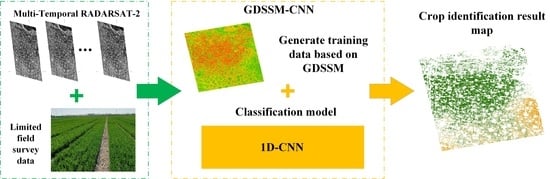
  • For multi-temporal and fully polarimetric SAR images, a crop classification method combining the geodesic distance spectral similarity measure and a one-dimensional convolution neural network (GDSSM-CNN) is proposed. This method can still have excellent classification ability when the sample is limited.
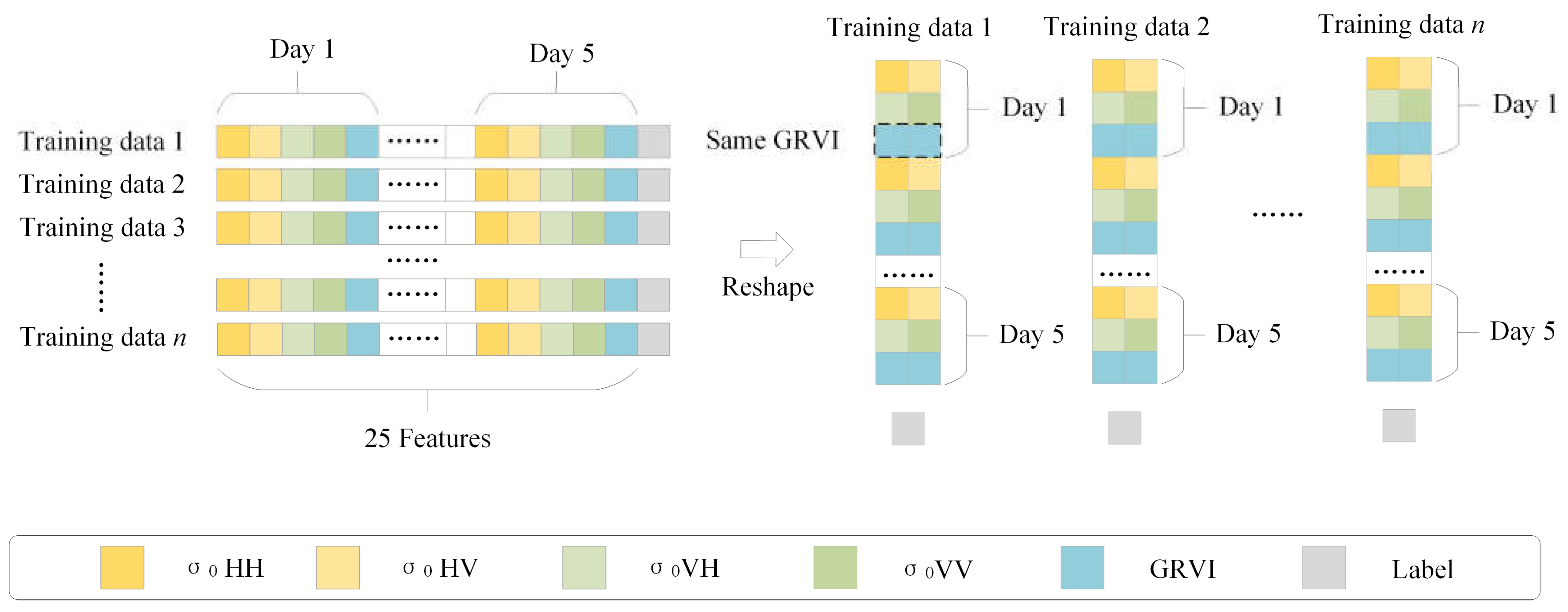
  • The backscatter coefficient and GRVI are extracted from multi-temporal and fully polarized images and combined.
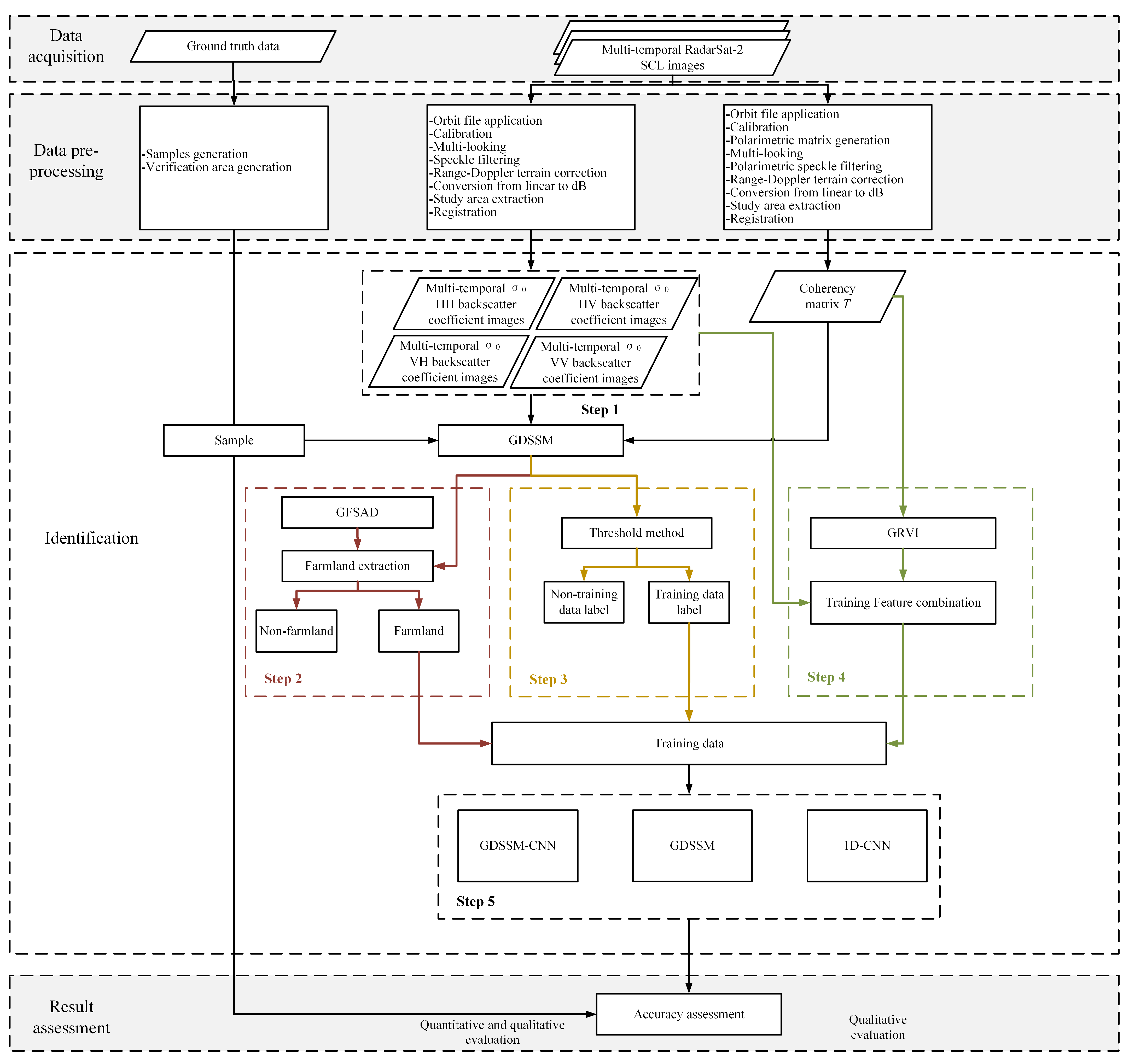
  • For multi-temporal and fully polarimetric SAR images, a farmland region extraction method combining GFSAD data and GDSSM is proposed. Farmland and non-farmland areas can be extracted by this method delicately.
The rest of this paper is arranged as follows: In Section 2, the research area, data and methodology are introduced. The experimental results of crop classification are given in Section 3. The discussion of the proposed method and its performance is introduced in Section 4. Section 5 concludes this paper.

2. Materials and Methods
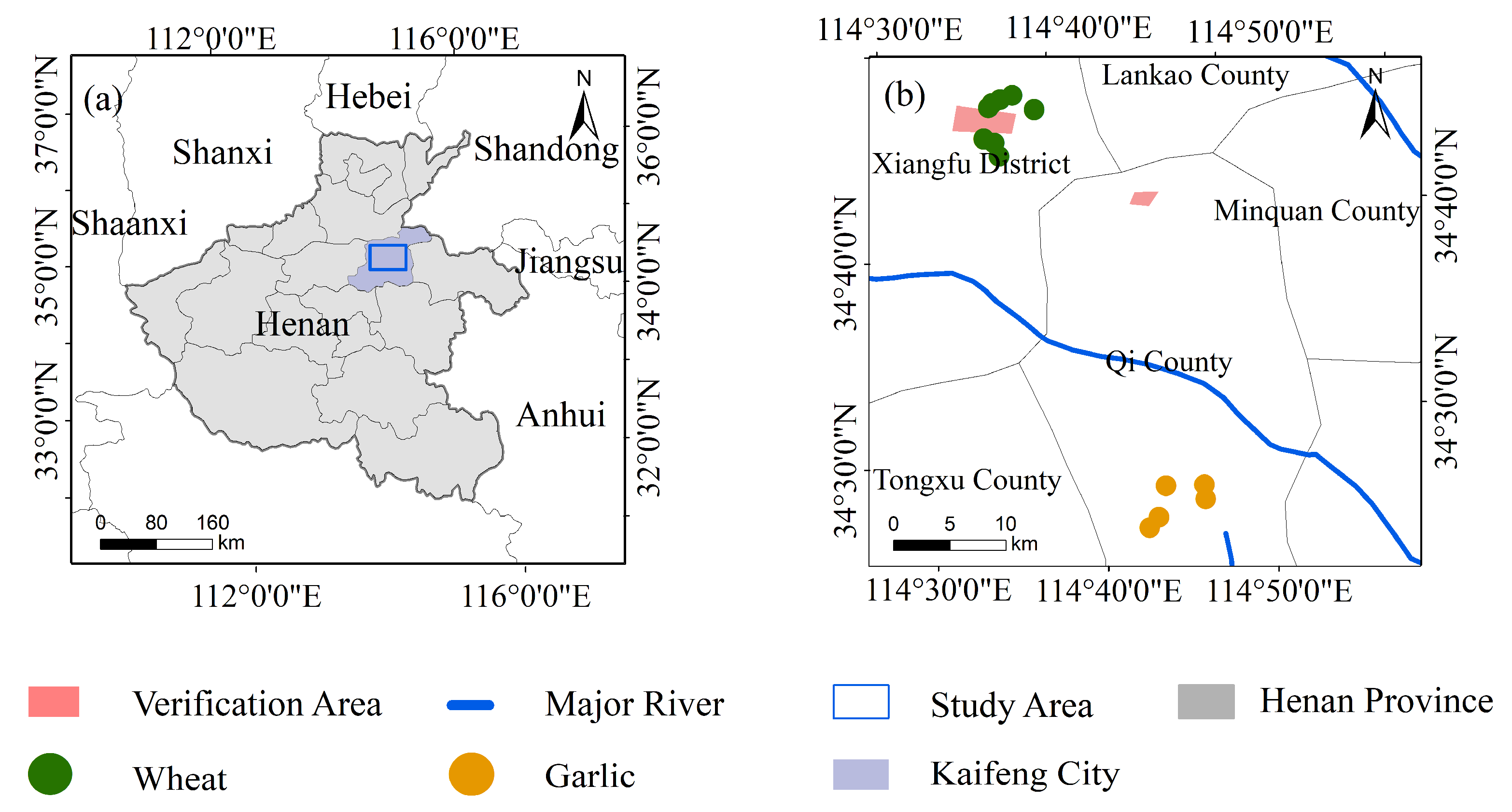
In this section, the materials and methods used for the experiments are described. Section 2.1 briefly introduces the study area, Section 2.2 describes the data used and the preprocessing of the data and Section 2.3 details the GDSSM-CNN method.

2.1. Study Area

The study area (114°27′40″E–114°48′57″E, 34°35′34″N–35°54′7″N) is located in the east of Kaifeng City, Henan Province, on the south bank of the Yellow River, as shown in Figure 1. Kaifeng has a temperate monsoon climate. It is cold and dry in winter and hot and humid in summer. The annual rainfall is 635 mm, and the annual average temperature (1981–2010) is 14.52 °C. Kaifeng is located on a plain with many rivers and moist soil, which is suitable for planting crops. In addition, Kaifeng City, with a farmland area of 3933 square kilometers and a total grain output of 3.06 million tons in 2021, is an important agricultural city in China. Crops are mainly divided into summer harvest crops and autumn harvest crops. In Kaifeng, summer harvest crops refer to the crops grown from October to June of the next year, mainly including winter wheat and a small amount of garlic; autumn harvest crops refer to crops grown from June to October, mainly including corn, peanuts and a small amount of rice and vegetables. This study focuses on summer crops; the planting area of winter wheat in 2021 was about 3098 square kilometers, and the garlic planting area was about 706 square kilometers.

2.2. Datasets and Preprocessing

RadarSat-2 is a ground imaging sensor equipped with C-band full polarimetric SAR [40]. It supports applications in various fields, including crop monitoring and pollution detection, target recognition and geological mapping. RadarSat-2 can perform imaging tasks all day, and the revisit cycle is 24 days. The specific parameters of the data are shown in Table 1. In this study, the RadarSat-2 data of SLC (Single Look Complex) of the fine quad polarization mode are used. The five-scene data of winter wheat growth in 2020 were obtained, which were 20 February, 15 March, 8 April, 2 May and 26 May, respectively. The time basically covered the complete life cycle of winter wheat from hibernation to maturity in the area.
RadarSat-2 data are preprocessed using the Sentinel Application Platform (SNAP) software provided by the European Space Agency (ESA) and The Environment for Visualizing Images (ENVI), a product of American Exelis Visual Information Solutions company. Pretreatment mainly includes the following: (1) orbit file application; (2) calibration, in which the backscattering coefficient of each pixel can be obtained; (3) polarimetric generation, in which the polarization coherency T matrix of each pixel can be obtained; (4) multi-looking; (5) refined Lee filtering; (6) range Doppler terrain correction; (7) conversion of the backscatter coefficient from linear to dB scale; (8) study area extraction; (9) registration. Each pixel in the multi-temporal SAR image corresponds to the same resolution unit. After preprocessing, ArcGIS software extracts the backscattering coefficient and polarization coherence matrix through the longitude and latitude coordinates of the sampling points.
The field survey data are essential information for crop classification and accuracy verification. In order to ensure the authenticity and accuracy of the ground field survey data, field surveys were conducted at the time of each satellite transit from July 2019 to June 2020 to collect and record the sample data of crops in the study area. During the field survey, Jisibao UG905 GPS (positioning accuracy is 1 to 3 m) was used outdoors to record the longitude and latitude information of the sampling point, and photos were taken to record the crop category information of the sampling point. Finally, 10 winter wheat sampling sites and 5 garlic sampling sites were randomly selected as samples. Two areas in the study area were selected randomly as the verification area through Google Earth software, and the types of crops in the verification area were determined through ground field investigation. The validation area contains 32,361 pixels in total, including 18,473 pixels for winter wheat, 6859 pixels for garlic and 7029 pixels for non-farmland areas. The distribution of the verification area and sampling points are shown in Figure 1a.

2.3. Methodology

The flow chart of this method is shown in Figure 2. The method combines the similarity calculation method GDSSM and the deep learning method 1D-CNN (GDSSM-CNN) to increase the number of training data and classify crops when the samples are limited. After collecting data and preprocessing, the method of crop type recognition is mainly divided into five steps. The first step is to calculate the GDSSM of pixels and samples, which can comprehensively compare the similarity of multi-temporal and fully polarimetric SAR data. In step 2, more refined farmland areas are extracted through the open farmland data GFSAD and GDSSM to prevent the interference of non-farmland factors. In step 3, the threshold method is used to extract the pixels that are very similar to the sample category as training data, which can fully train the neural network when the samples are very limited. In step 4, the GRVI of the pixel is calculated and combined with the backscatter coefficient as the feature. GRVI reflects the physical scattering characteristics and phenological characteristics of crops and can improve the performance and efficiency of classification. In step 5, the 1D-CNN neural network model is used for training, which can effectively extract the features of multi-temporal data. Finally, the classification results of the model are analyzed and verified.

2.3.1. Geodesic Distance Spectral Similarity Measure

GDSSM (shown in Equation (8)) defines the similarity between the reference target and unknown pixels; it is composed of geodesic distance similarity (GDS) (shown in Equations (1)–(3)), spectral correlation similarity (SCS) (shown in Equations (4) and (5)) and Euclidean distance similarity (EDS) (shown in Equations (6) and (7)). The specific descriptions of SCS and EDS appear in [41,42], and the specific description of GDS appears in [29]. GDS compares the scattering similarity of the polarization coherence matrix T of a reference target and an unknown pixel. In the polarization scattering theory, the Kennaugh matrix of the scattering of incoherent targets reflects the dependence of the radar received power on the transceiver antenna, which is shown by the coherence matrix T:
K = T 11 + T 22 + T 33 2 ( T 12 ) ( T 13 ) ( T 23 ) ( T 12 ) T 11 + T 22 T 33 2 ( T 23 ) ( T 13 ) ( T 13 ) ( T 23 ) T 11 T 22 + T 33 2 ( T 12 ) ( T 23 ) ( T 13 ) ( T 12 ) T 11 + T 22 + T 33 2
where and represent the real and imaginary parts of the complex number. The geodesic distance similarity value (GDSV) describes the similarity of geodesic distances between two Kennaugh matrices on the unit sphere. The equation used to calculate GDSV is as follows:
GDSV = GD K p , K q = 2 π c o s 1 T r K q T K p T r K q T K q T r K p T K p
where K p and K q denote the unknown pixel Kennaugh matrix and reference target Kennaugh matrix, respectively. T r represents the matrix trace, K T represents the transposition of the of pixel Kennaugh matrix, and the range of GDSV is [0, 1]. GDS is the average of GDSV for five dates. The equation used to calculate GDS is as follows:
GDS = 1 n i = 1 n GDSV i = 1 n i = 1 n GD K p i , K q i
where n is the number of Radarsat-2 data images, K p i and K q i are the Kennaugh matrices of unknown pixel and reference target in the image, respectively.
SCS and EDS compare the similarity of backscattering coefficient vectors of a reference target and an unknown pixel. The objects of SCS and EDS are the spectral information in optical remote sensing. However, in this study, the multi-phase characteristics of the backscattering coefficient are used to replace the spectral information; that is, the fully polarized backscattering coefficient at a certain time represents a spectral value. The multi-temporal fully polarized backscattering coefficient of each crop in the sample set is used as the vector of the reference target. The multi-temporal backscattering coefficient of a pixel in the dataset to be classified is taken as the vector of the unknown target. The equation used to calculate SCS is as follows:
SCS orig = 1 n 1 i = 1 n P i μ P ( Q i μ Q ) σ P σ Q
and
SCS = SCS orig m s M s m s
where μ and σ are the mean and standard deviation of the vector; P and Q are the backscattering coefficient vectors of the unknown pixel and the reference pixel, respectively; and P i and Q i are the backscattering coefficients of the unknown pixel and the reference pixel at a certain time, respectively. m s and M s are the minimum and maximum values of SCS orig . The range of SCS is [0, 1]. The larger the value, the more similar the reference pixel is to the target pixel.
The Euclidean distance measure is used to measure the degree of separation or proximity between two vectors. The equation used to calculate EDS is as follows:
E d orig = i = 1 n P i Q i 2
and
EDS = Ed orig m E M E m E
where m E and M E are the minimum and maximum values of Ed orig , respectively. The range of EDS is [0, 1]. The smaller the value, the more similar the reference pixel is to the target pixel. GDSSV is composed of GDS, SCS and EDS, and its equation is as follows:
GDSSV = SCS 2 + 1 Ed 2 × GDS
The range of GDSSV is [0, 1]. The larger the GDSSV, the more similar the unknown pixel is to the reference pixel. When the GDSSV of a pixel and the reference pixel is greater than 0.80, it is considered that the unknown pixel and the reference pixel belong to the same category of crops.

2.3.2. Generalized Volume Scattering Model-Based Radar Vegetation Index

GRVI describes the similarity between Kennaugh matrix K and generalized volume scattering model K v of pixels. It has been proved to have the potential to monitor the growth of rice at different phenological stages [29,30]. K v is related to the generalized volume scattering model [43], which is shown as follows:
K v = 1 3 1 + γ 4 γ 6 3 2 1 + γ γ 3 γ 1 0 0 γ 1 1 2 1 + γ + γ 3 0 0 0 0 1 2 1 + γ + γ 3 0 0 0 0 1 2 1 + γ γ
where γ indicates the co-polarized ratio. Geodesic distance f v between K and K v is as follows:
f v = 1 GD K , K v
where GD describes the geodesic distance between two Kennaugh matrices. GRVI (shown in Equation (2)) is composed of geodesic distance f v and modulation parameters β . The equation used to calculate GRVI and β is as follows:
β = p q 2 G D K , K v
p = min GD K , K t GD K , K c GD K , K d GD K , K n d , q = max GD K , K t GD K , K c GD K , K d GD K , K n d
GRVI = β f v
where p and q are the minimum and maximum geodesic distances between K and elementary targets, respectively. K t is the Kennaugh matrix of a trihedral; K c is the Kennaugh matrix of a cylinder; K d is the Kennaugh matrix of a dihedral; K n d is the Kennaugh matrix of a narrow dihedral. This Kennaugh matrix of elementary targets is shown in the work of Ratha et al. [44].

2.3.3. Farmland Extraction

Since the scattering characteristics of the non-farmland area are so complicated, it is possible that parts of the structure and scattering characteristics of crops at different growth stages are similar to those of non-farmland areas, which could lead to incorrect results in the classification findings. In this study, the open dataset GFSAD is used to provide a farmland mask with a resolution of 30 m. It has been widely used in various agricultural applications [45]: farmland type identification, spatial and temporal changes in farmland extent, cropping intensities, etc. However, farmland and villages in Kaifeng are distributed in a scattered way, so there are only dense non-farmland areas such as villages, roads and waters in GFSAD, and many small roads and scattered buildings have not been identified. Unknown pixels with GDSSM similarity less than 0.3 for all crop categories are marked as non-farmland pixels. These non-farmland pixel sets in GDSSM and non-farmland pixel sets in GFSAD form the non-farmland areas in the study area, which are shown as follows:
N F = N F GDSSM N F GFSAD
where N F G D S S M and N F G F S A D are the sets of non-farmland pixels in GDSSM and GFSAD, respectively. N F is the set of non-farmland pixels in the study area.
The farmland mask can be obtained by removing all non-farmland areas in the study area, which is shown as follows:
F M = S M N F
where S M is the set of all pixels in the study area. F M is the set of all farmland pixels in the study area. This method, which combines the geodesic distance spectral similarity measure and GFSAD data, can accurately extract the farmland and non-farmland areas in the study area and finally remove the non-farmland areas in the study area.

2.3.4. Training Data Extraction

Deep learning models usually require sufficient data training. Because the dataset of SAR image is less than that of natural scene and SAR image is very sensitive to the incident angle and other information, current optical images and data enhancement operations used in natural scenes are not reasonable for SAR images [46]. The crops planted in different areas may have large morphological differences. For example, the wheat in Henan Province is generally 80 cm high after ripening, while the wheat in Zhejiang Province is generally 65 cm high after ripening. Due to the morphological differences between crops, transfer learning, meta-learning and other sample migration methods are not suitable for crop applications. In this study, GDSSM and the threshold method are used to obtain a large number of samples. GDSSM describes the similarity between the reference target and unknown pixels. The larger the value, the more similar the two pixels are. When the GDSSM of the unknown pixel and the reference pixel is greater than the threshold, the unknown pixel is regarded as the same training data as the reference target category. Through the threshold method, a large number of training data can be selected, which can be used for the training of the neural network. In order to ensure that the training data and samples have a very high degree of similarity, the threshold value needs to be greater than or equal to 0.8. Finally, four thresholds are selected, namely 0.95, 0.9, 0.85 and 0.8, and the effects of different thresholds on classification results are compared.

2.3.5. One-Dimensional Convolutional Neural Network

In order to make effective use of the information in multi-temporal and fully polarimetric SAR images, the backscatter coefficients and GRVI of the four polarization modes are combined into features in the order of HH, HV, VH, VV and GRVI. These combined features are arranged according to the time of five SAR images. In order to use feature combinations effectively, a convolution neural network (CNN) model is used to classify crops. The convolutional neural network is a widely used method in deep learning and has been applied in various applications of agricultural remote sensing. It has been proved to have excellent feature extraction ability. Among CNNs, the one-dimensional convolutional neural network model has more advantages in analyzing sequence characteristic data [47]. Three convolutional filters are set in the 1D-CNN model. Three-layer convolution can comprehensively extract the features of sequence data integration. The maximum pool layers and batch normalization layers are set after the convolution layer, which can reduce the size of the model and improve the calculation speed. Finally, the dimension of the data is transformed by using the flatten layer, and the data are sent to the Softmax layer for classification. The 1D-CNN model is created through the Keras framework.
A RadarSat-2 image has four polarizations. Five features can be obtained from each SAR image. They are four backscattering coefficients (σ0 HH, σ0 HV, σ0VH and σ0 VV) and a generalized volume scattering model based on radar vegetation index. Since five RadarSat-2 images at different times are used, the characteristic shape of each sample is (1, 25). To facilitate the input of samples into the 1D-CNN model, the GRVI values of five dates are copied, filled into the features and reshaped. The shape of each sample changes to (15, 2), as shown in Figure 3.
The 1D-CNN model is used to identify crop types. The detailed parameters of 1D-CNN are shown in Figure 4. By using the training data obtained by GDSSM, the trained 1D-CNN model is used to classify the crops in the study area.

3. Results

To evaluate the proposed method, this section will present the results of the experiments. Firstly, Section 3.1 presents the backscattering coefficients and GRVI for multi-temporal phases. Section 3.2 presents GDSSM for different crops. After that, Section 3.3 shows the farmland masks obtained by the GDSSM method. Finally, Section 3.4 presents the classification results of different methods.

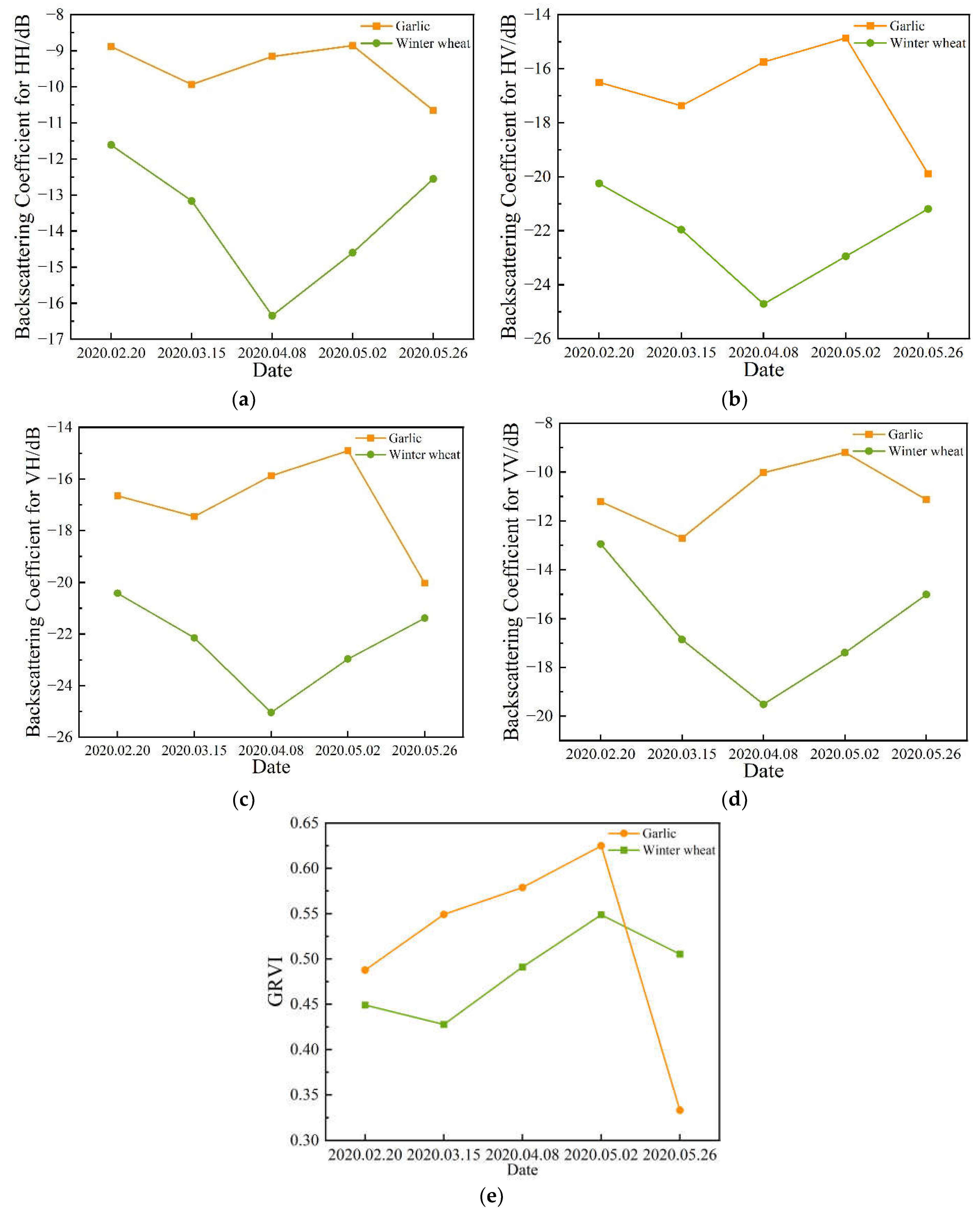
3.1. Temporal Profiles of the Backscatter Coefficient and GRVI

The backscattering coefficient represents the reflectivity of the target unit cross-sectional area in the incident direction of the radar electromagnetic wave and can reflect the geometric and physical characteristics of the illuminated object, such as surface roughness and water content, which can help identify the types of crops. Figure 5 shows the time profile of four polarization modes, where the value of each point represents the average backscatter coefficient of each crop type sample.
The radar vegetation index based on the generalized lifting scattering model is a vegetation index that reflects the scattering mechanism of crops. The vegetation index changes with the growth and development of crops and has been proved to have potential in rice monitoring. This parameter is helpful in classifying crops. Figure 5 shows the time profile of GRVI, where the value of each point represents the average GRVI for each crop type sample.

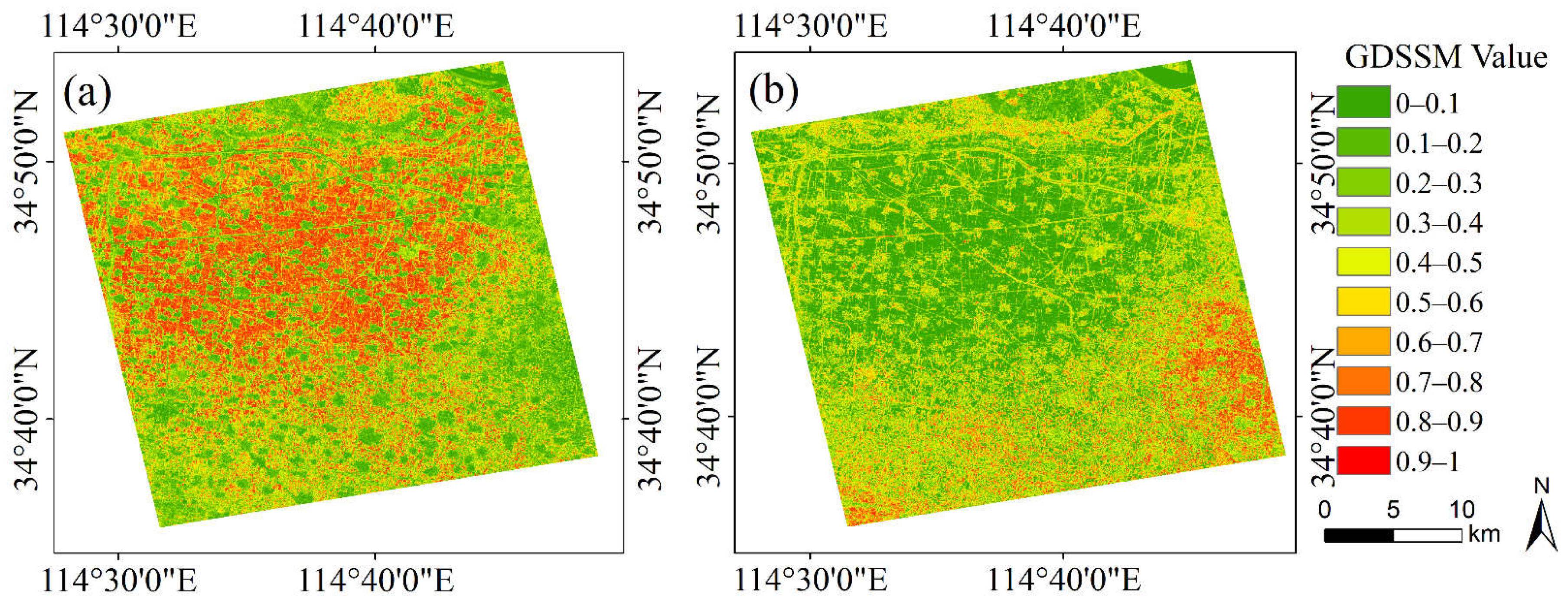
3.2. GDSSM for Different Crops
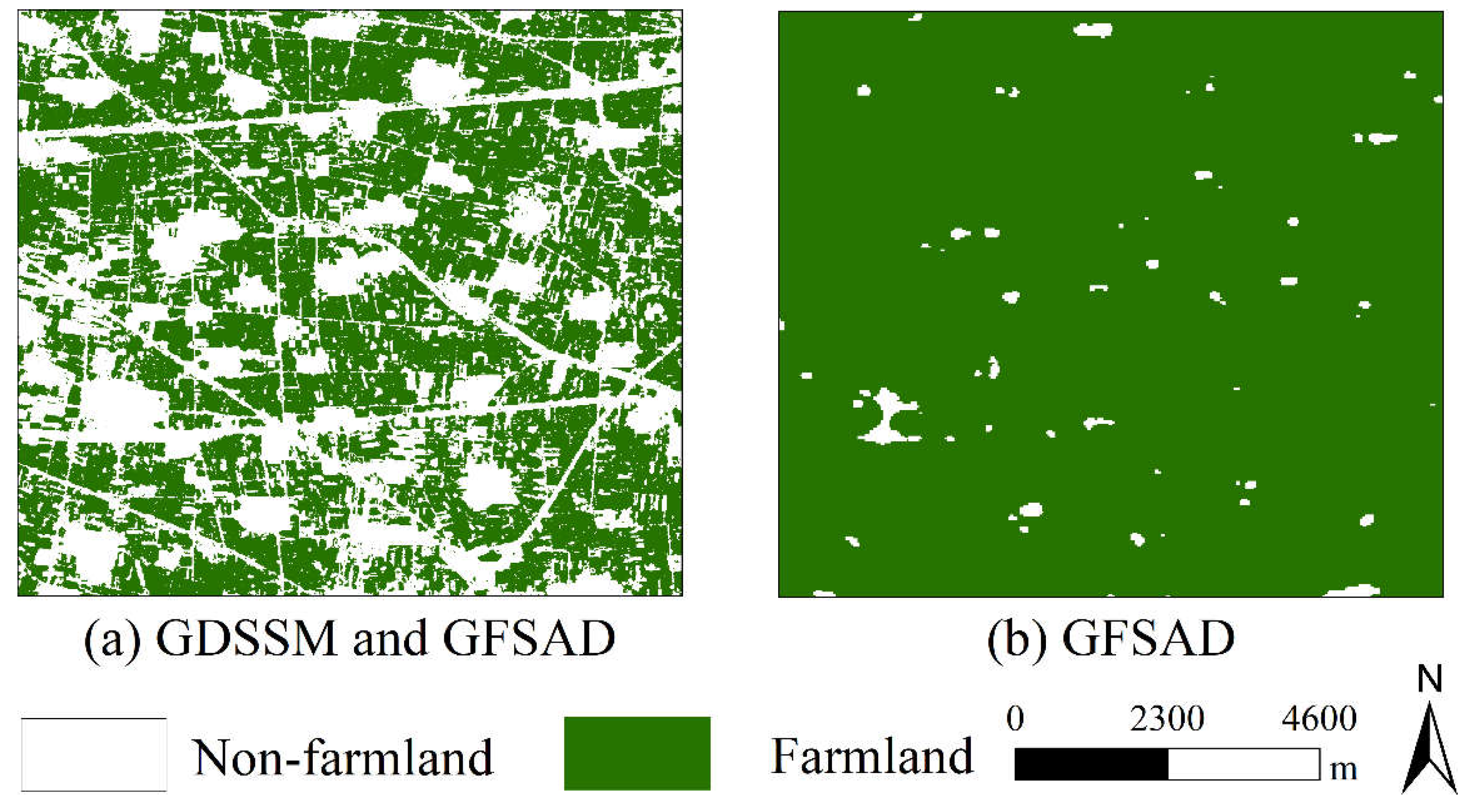
Figure 6 shows the GDSSM between unknown pixels and winter wheat samples and between unknown pixels and garlic samples in the study area. As can be seen from Figure 6, GDSSM values of non-farmland pixels such as towns and paths are very low (within a range of 0–0.4). In Figure 6a, the farmland mainly planted with winter wheat has a very high GDSSM with the winter wheat sample (within a range of 0.8–1), while the farmland mainly planted with garlic has a very low GDSSM with the winter wheat sample (within a range of 0–0.2). The opposite is true in Figure 6b. Areas where winter wheat and garlic are grown were identified during the field visit. This proves that GDSSM can accurately show the similarity between unknown pixels and reference samples and is very helpful for distinguishing crop types and farmland and non-farmland areas. Moreover, it is proved that when GDSSM is greater than or equal to 0.8, the unknown pixel has a very high similarity with the reference sample, which is conducive to selecting the pixel with high similarity as the training data.

3.3. Farmland Mask

The extraction results of the farmland mask in some study areas and the mask of GFSAD are shown in Figure 7. It can be seen from the figure that GFSAD only contains a few dense buildings and large villages. After combining GDSSM, many paths and scattered buildings are identified. The reason may be that the paths are very narrow and the image resolution is very low, resulting in a path and a small part of the farmland beside the road being in the same pixel. Through the GDSSM method, it can be judged that the similarity between these mixed pixels and crops is not high, allowing the identification of paths and discrete buildings. This fully shows that the farmland extraction method of GDSSM can identify smaller non-farmland areas and finer farmland areas.

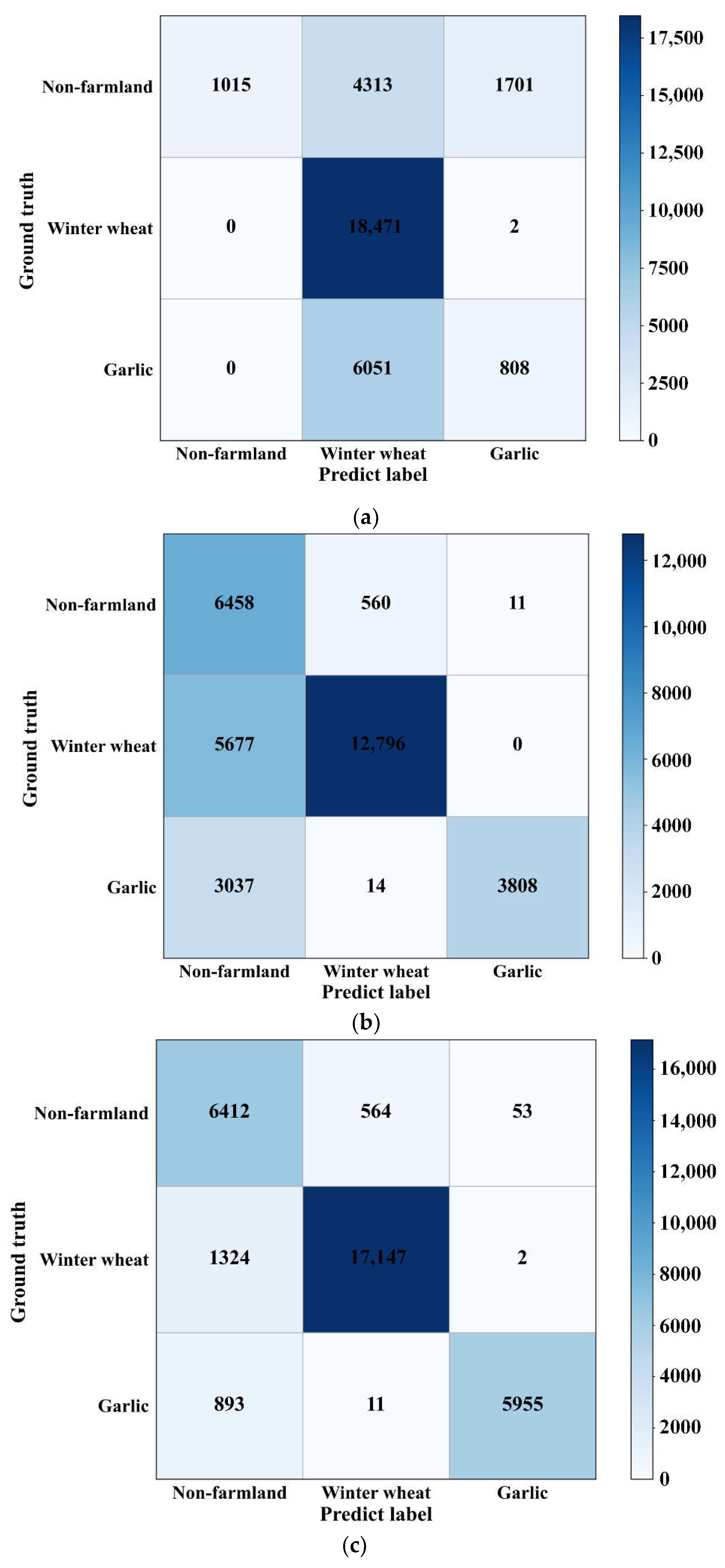
3.4. Crop Classification

In order to prove the effectiveness of the model combining geodesic distance spectral similarity measure and one-dimensional convolutional neural network (GDSSM-CNN), the crop recognition method using GDSSM and the crop recognition method using the 1D-CNN model are compared. The use of similarity and threshold methods to classify crops has been proved to have a good effect [48,49]. In addition, in order to study the influence of different thresholds (in the training data generation part) on the classification results, GDSSM-CNN methods with thresholds of 0.95, 0.9, 0.85 and 0.8 are used for comparison. Pixels whose threshold value is greater than or equal to 0.8 are considered to have very high similarities with reference samples (shown in Section 4.2). Therefore, only thresholds greater than or equal to 0.8 are used.
In order to compare the performance of various methods more precisely, the output results of each model and the ground data labels are generated into a confusion matrix for analysis, as shown in Figure 8. From these confusion matrices, it can be seen that GDSSM-CNN models show high accuracy, while the accuracy of using 1D-CNN and GDSSM methods alone is very low. The results are presented in Table 2. The GDSSM-CNN method with a threshold of 0.8 for training data has the highest accuracy, with an accuracy rate of 91.20% and a Kappa coefficient of 0.8509. Experiments show that the combined performance of the GDSSM classifier and 1D-CNN classifier is better than that of either of them alone. The accuracy increased by 19.94% and 23.91%, respectively, and the Kappa coefficient increased by 0.3018 and 0.5497, respectively.
In order to intuitively prove the differences between methods, some classification results are used for comparison, and the comparison results shown in Figure 9 and Figure 10 show the final classification results of the study area obtained by the GDSSM-CNN model.

4. Discussion

To demonstrate the superiority of the GDSSM-CNN method, this section will discuss the results. Firstly, Section 4.1 discusses the need to combine the backscatter coefficient and GRVI. After that, Section 4.2 explores the effect of different amounts of training data on the classification results. Finally, the performance of the three methods is discussed in Section 4.3.

4.1. Combination of Backscatter Coefficient and GRVI

By analyzing the backscattering coefficients of garlic and winter wheat, it can be seen that the backscattering coefficient of winter wheat is always smaller than that of garlic. From 15 March to 2 May, the backscattering coefficient of winter wheat is significantly different from that of garlic, because during this period, the length of winter wheat increases rapidly and the morphology changes significantly. However, the backscattering coefficients of winter wheat and garlic are very close at some times, such as those on 20 February and 26 May, which means that it is difficult to distinguish crops by only using backscattering coefficients.
Through the analysis of GRVI of garlic and winter wheat, it can be seen that GRVI of winter wheat and garlic both show an upward trend with the growth of crops, but there is little difference between GRVI values of winter wheat and garlic from 20 February to 2 May, which means that it is difficult to distinguish crops by only using GRVI. Different from the backscattering coefficients, the GRVI values of winter wheat and garlic differ greatly on 26 May, which is caused by the harvesting of garlic. The backscattering coefficient and GRVI provide two different kinds of information, which is very necessary. This not only shows that combining the backscatter coefficient and GRVI can be beneficial in identifying crops but also shows the importance of using multi-temporal features. In order to better identify crops, the backscatter coefficient and GRVI are combined in the study.

4.2. Extraction of Training Data

In order to explore the impact of the number of training data on the performance of the classifier, the number of training data generated by different thresholds and the classification accuracy are compared, as shown in Table 3. By analyzing Table 3, it can be found that:
  • From the number of training data, it can be seen that the number of training data increases rapidly with the decrease in the threshold, and the model training time increases rapidly with the increase in the amount of training.
  • From the number of training data and the accuracy of the classifier, it can be seen that the accuracy of the classifier increases with the increase in training data. When the threshold is 0.9, the increase in training data has little impact on the accuracy. This means that the 1D-CNN model has been fully trained by the training data at this time.
  • As the number of training data increases, the number of noise data (training data with wrong labels) increases. However, the accuracy of the classifier becomes higher and higher. This means that when the threshold is greater than or equal to 0.8, the number of noisy data is far less than the number of training data with correct labels, and the increase in low-noise data does not affect the performance of the classifier. When the threshold value is less than 0.8, the unknown pixel does not have a high similarity with the reference target. Therefore, when the threshold value is in the range of 0.8–0.9, the classifier can achieve very high accuracy.

4.3. Comparison of Three Methods

By analyzing the confusion matrix, it can be found that the user’s accuracy for non-farmland area is very low in the results using the GDSSM method. The reason is that when only the threshold method is used for classification, the classification performance is affected by the selection of threshold, the proportion of mixed pixels, and image noise, which is also reflected in other classification results of the GDSSM model. In the results using the 1D-CNN method, the user’s accuracy and producer’s accuracy for garlic are very low. The reason for this result is that the sample size is too small, which makes the model unable to fully learn the types of crops in the training stage. The GDSSM-CNN model has very high user accuracy and producer accuracy, which proves that this model also has very good performance when there is a limited number of samples.
From the difference diagram of the classification results of the three methods, it can be clearly seen that the effect of the GDSSM-CNN model is better than that of other models. In area A, the GDSSM model mistakenly identifies farmland as non-farmland. The 1D-CNN model mistakenly identifies non-farmland as garlic and does not identify some paths. The reason is that the model training is inadequate due to insufficient samples. Many farmlands in the GDSSM-CNN model are correctly identified, which proves that the GDSSM-CNN method has better identification ability and is rarely affected by the number of samples. In area B, the GDSSM model can distinguish the areas where wheat and garlic are mixed, but it still recognizes much farmland as non-farmland. A large amount of garlic was incorrectly identified as winter wheat by the 1D-CNN model. The GDSSM-CNN model still has very good classification results in the area where winter wheat and garlic are mixed, which means that the GDSSM model can select the correct pixels as training data, thus improving the performance of the 1D-CNN. It can be seen from Figure 10 that the planting area of winter wheat gradually shrinks from north to south (shown in the red rectangular boxes in Figure 10), and garlic is mainly planted in the southeast and southwest of the study area (shown in the blue rectangular boxes in Figure 10). The southern part of the study area is mainly planted with winter wheat and garlic (shown in the black circle in Figure 10). Through comparison with optical images, these planting distributions are confirmed.
Based on the analysis and verification of classification results, the following conclusions can be drawn: The GDSSM model can identify winter wheat and garlic, and it is less affected by the limited samples. However, the classification performance of this model is subpar. The 1D-CNN model has a strong feature extraction ability, but the number of samples easily limits its performance. The GDSSM-CNN model, which combines the two models, not only is free from the limitation of the number of samples but also has very high accuracy and robustness.

5. Conclusions

In this study, a crop classification method based on GDSSM-CNN is proposed. This method uses multi-temporal RadarSat-2 images, and the performance of the classifier is not limited by the number of samples. The details are as follows: Firstly, the geodesic distance spectral similarity between unknown pixels and crop samples is calculated. Secondly, GDSSM is used in combination with the disclosed GFSAD farmland mask to remove non-farmland areas and is compared with the GFSAD mask only. Thirdly, backscatter coefficients and GRVI features are extracted from multi-temporal images and combined to generate crop classification models. Fourthly, GDSSM and the threshold method are used to extract unlabeled data with very high similarity with samples as training data, and the effects of different thresholds are compared. The optimal threshold selection range is determined to be 0.8–0.9. Finally, the GDSSM classifier combining GDSSM and 1D-CNN is used to train the model using the feature combination of backscatter coefficient and GRVI.
GDSSM, 1D-CNN and GDSSM-CNN models with different thresholds were used for comparison. Only 10 winter wheat samples and 5 garlic samples were used. The GDSSM-CNN method shows strong crop classification performance. The accuracy of the GDSSM-CNN method with different thresholds is above 89%, which is higher than that of the GDSSM method (the accuracy is 71.26%) and 1D-CNN method (the accuracy is 67.29%), which proves the accuracy of the GDSM-CNN method. Some classification results were selected for comparison, proving that the GDSSM-CNN method has a satisfactory classification effect. In a word, analysis and verification of three methods have proved that the GDSSM-CNN model has incomparable advantages in crop classification.
In addition, the combination of backscatter coefficient and GRVI has proved to be very useful for crop classification results. In addition, compared with the non-farmland mask only using GFSAD, the non-farmland mask added with GDSSM can more finely identify small-scale buildings and roads. This study shows that the use of rich polarization information and multi-temporal SAR images brings new possibilities to crop classification and also provides a new idea for the sample size limitation of neural networks in SAR image applications.

Author Contributions

Conceptualization, H.L., G.T. and N.L.; data curation, H.Y., J.L. and N.L.; investigation, H.L., G.T., J.Z. and N.L.; methodology, H.L., G.T. and H.Y.; supervision, H.L., J.Z. and N.L.; writing—original draft, H.L., J.L. and N.L.; writing—review and editing, H.L., G.T. and N.L. All authors have read and agreed to the published version of the manuscript.

Funding

This research was funded by the National Natural Science Foundation of China (42101386), the College Key Research Project of Henan Province (22A520021, 21A520004), the Plan of Science and Technology of Henan Province (212102210093, 222102110439) and the Plan of Science and Technology of Kaifeng City (2102005).

Data Availability Statement

All data and model presented in this study are available.

Acknowledgments

The authors would like to thank NASA for providing Global Food Security-Support Analysis Data at 30 m.

Conflicts of Interest

The authors declare no conflict of interest.

References

  1. Kwak, G.-H.; Park, N.-W. Impact of texture information on crop classification with machine learning and UAV images. Appl. Sci. 2019, 9, 643. [Google Scholar] [CrossRef]
  2. Zhong, L.; Hu, L.; Zhou, H. Deep learning based multi-temporal crop classification. Remote Sens. Environ. 2019, 221, 430–443. [Google Scholar] [CrossRef]
  3. Yang, H.; Li, H.; Wang, W.; Li, N.; Zhao, J.; Pan, B. Spatio-temporal estimation of rice height using time series Sentinel-1 images. Remote Sens. 2022, 14, 546. [Google Scholar] [CrossRef]
  4. Xie, Y.; Huang, J. Integration of a crop growth model and deep learning methods to improve satellite-based yield estimation of winter wheat in Henan Province, China. Remote Sens. 2021, 13, 4372. [Google Scholar] [CrossRef]
  5. Pôças, I.; Calera, A.; Campos, I.; Cunha, M. Remote sensing for estimating and mapping single and basal crop coefficientes: A review on spectral vegetation indices approaches. Agric. Water Manag. 2020, 233, 106081. [Google Scholar] [CrossRef]
  6. Sun, C.; Bian, Y.; Zhou, T.; Pan, J. Using of multi-source and multi-temporal remote sensing data improves crop-type mapping in the subtropical agriculture region. Sensors 2019, 19, 2401. [Google Scholar] [CrossRef]
  7. Shi, S.; Ye, Y.; Xiao, R. Evaluation of food security based on remote sensing data—Taking Egypt as an example. Remote Sens. 2022, 14, 2876. [Google Scholar] [CrossRef]
  8. Leroux, L.; Castets, M.; Baron, C.; Escorihuela, M.-J.; Bégué, A.; Lo Seen, D. Maize yield estimation in West Africa from crop process-induced combinations of multi-domain remote sensing indices. Eur. J. Agron. 2019, 108, 11–26. [Google Scholar] [CrossRef]
  9. Sun, Y.; Luo, J.; Wu, T.; Zhou, Y.; Liu, H.; Gao, L.; Dong, W.; Liu, W.; Yang, Y.; Hu, X.; et al. Synchronous response analysis of features for remote sensing crop classification based on optical and SAR time-series data. Sensors 2019, 19, 4227. [Google Scholar] [CrossRef]
  10. Li, C.; Li, H.; Li, J.; Lei, Y.; Li, C.; Manevski, K.; Shen, Y. Using NDVI percentiles to monitor real-time crop growth. Comput. Electron. Agric. 2019, 162, 357–363. [Google Scholar] [CrossRef]
  11. French, A.N.; Hunsaker, D.J.; Sanchez, C.A.; Saber, M.; Gonzalez, J.R.; Anderson, R. Satellite-Based NDVI crop coefficients and evapotranspiration with eddy covariance validation for multiple durum wheat fields in the US Southwest. Agric. Water Manag. 2020, 239, 106266. [Google Scholar] [CrossRef]
  12. Wei, S.; Zhang, H.; Wang, C.; Wang, Y.; Xu, L. Multi-temporal SAR data large-scale crop mapping based on U-Net model. Remote Sens. 2019, 11, 68. [Google Scholar] [CrossRef]
  13. Adrian, J.; Sagan, V.; Maimaitijiang, M. Sentinel SAR-Optical fusion for crop type mapping using deep learning and Google Earth Engine. ISPRS J. Photogramm. Remote Sens. 2021, 175, 215–235. [Google Scholar] [CrossRef]
  14. Bouchat, J.; Tronquo, E.; Orban, A.; Verhoest, N.E.C.; Defourny, P. Assessing the potential of fully polarimetric Mono- and bistatic SAR acquisitions in L-Band for crop and soil monitoring. IEEE J. Sel. Top. Appl. Earth Obs. Remote Sens. 2022, 15, 3168–3178. [Google Scholar] [CrossRef]
  15. Nasirzadehdizaji, R.; Balik Sanli, F.; Abdikan, S.; Cakir, Z.; Sekertekin, A.; Ustuner, M. Sensitivity analysis of multi-temporal Sentinel-1 SAR parameters to crop height and canopy coverage. Appl. Sci. 2019, 9, 655. [Google Scholar] [CrossRef]
  16. Wang, H.; Magagi, R.; Goïta, K.; Trudel, M.; McNairn, H.; Powers, J. Crop phenology retrieval via polarimetric SAR decomposition and random forest algorithm. Remote Sens. Environ. 2019, 231, 111234. [Google Scholar] [CrossRef]
  17. Xu, L.; Zhang, H.; Wang, C.; Zhang, B.; Liu, M. Crop classification based on temporal information using Sentinel-1 SAR time-series data. Remote Sens. 2019, 11, 53. [Google Scholar] [CrossRef]
  18. Gao, H.; Wang, C.; Wang, G.; Fu, H.; Zhu, J. A novel crop classification method based on PpfSVM Classifier with time-series alignment kernel from dual-polarization SAR datasets. Remote Sens. Environ. 2021, 264, 112628. [Google Scholar] [CrossRef]
  19. Liao, C.; Wang, J.; Xie, Q.; Baz, A.A.; Huang, X.; Shang, J.; He, Y. Synergistic use of multi-temporal RADARSAT-2 and VENµS data for crop classification based on 1D convolutional neural network. Remote Sens. 2020, 12, 832. [Google Scholar] [CrossRef]
  20. Xie, Q.; Lai, K.; Wang, J.; Lopez-Sanchez, J.M.; Shang, J.; Liao, C.; Zhu, J.; Fu, H.; Peng, X. Crop monitoring and classification using polarimetric RADARSAT-2 time-series data across growing season: A case study in Southwestern Ontario, Canada. Remote Sens. 2021, 13, 1394. [Google Scholar] [CrossRef]
  21. Li, M.; Bijker, W. Vegetable classification in indonesia using dynamic time warping of Sentinel-1A dual polarization SAR time series. Int. J. Appl. Earth Obs. Geoinf. 2019, 78, 268–280. [Google Scholar] [CrossRef]
  22. Yamaguchi, Y.; Moriyama, T.; Ishido, M.; Yamada, H. Four-Component scattering model for polarimetric SAR image decomposition. IEEE Trans. Geosci. Remote Sens. 2005, 43, 1699–1706. [Google Scholar] [CrossRef]
  23. Singh, G.; Yamaguchi, Y. Model-based six-component scattering matrix power decomposition. IEEE Trans. Geosci. Remote Sens. 2018, 56, 5687–5704. [Google Scholar] [CrossRef]
  24. Singh, G.; Malik, R.; Mohanty, S.; Rathore, V.S.; Yamada, K.; Umemura, M.; Yamaguchi, Y. Seven-component scattering power decomposition of POLSAR coherency matrix. IEEE Trans-Actions Geosci. Remote Sens. 2019, 57, 8371–8382. [Google Scholar] [CrossRef]
  25. Guo, J.; Wei, P.-L.; Liu, J.; Jin, B.; Su, B.-F.; Zhou, Z.-S. Crop classification based on differential characteristics of H/α scattering parameters for multitemporal Quad- and Dual-Polarization SAR images. IEEE Trans. Geosci. Remote Sens. 2018, 56, 6111–6123. [Google Scholar] [CrossRef]
  26. Chen, Q.; Cao, W.; Shang, J.; Liu, J.; Liu, X. Superpixel-based cropland classification of SAR image with statistical texture and polarization features. IEEE Geosci. Remote Sens. Lett. 2022, 19, 1–5. [Google Scholar] [CrossRef]
  27. Ratha, D.; Bhattacharya, A.; Frery, A.C. Unsupervised classification of PolSAR data using a scattering similarity measure derived from a geodesic distance. IEEE Geosci. Remote Sens. Lett. 2018, 15, 151–155. [Google Scholar] [CrossRef]
  28. Phartiyal, G.S.; Kumar, K.; Singh, D. An improved land cover classification using polarization signatures for PALSAR 2 data. Adv. Space Res. 2020, 65, 2622–2635. [Google Scholar] [CrossRef]
  29. Mandal, D.; Kumar, V.; Ratha, D.; Lopez-Sanchez, J.M.; Bhattacharya, A.; McNairn, H.; Rao, Y.S.; Ramana, K.V. Assessment of rice growth conditions in a semi-arid region of india using the generalized radar vegetation index derived from RADARSAT-2 polarimetric SAR data. Remote Sens. Environ. 2020, 237, 111561. [Google Scholar] [CrossRef]
  30. Ratha, D.; De, S.; Celik, T.; Bhattacharya, A. Change detection in polarimetric SAR images using a geodesic distance between scattering mechanisms. IEEE Geosci. Remote Sens. Lett. 2017, 14, 7. [Google Scholar] [CrossRef]
  31. Xie, Q.; Dou, Q.; Peng, X.; Wang, J.; Lopez-Sanchez, J.M.; Shang, J.; Fu, H.; Zhu, J. Crop classification based on the physically constrained general model-based decomposition using multi-temporal RADARSAT-2 Data. Remote Sens. 2022, 14, 2668. [Google Scholar] [CrossRef]
  32. Small, D. Flattening gamma: Radiometric terrain correction for SAR Imagery. IEEE Trans. Geosci. Remote Sens. 2011, 49, 3081–3093. [Google Scholar] [CrossRef]
  33. Orynbaikyzy, A.; Gessner, U.; Conrad, C. Spatial transferability of random forest models for crop type classification using Sentinel-1 and Sentinel-2. Remote Sens. 2022, 14, 1493. [Google Scholar] [CrossRef]
  34. Liu, Y.; Zhao, W.; Chen, S.; Ye, T. Mapping crop rotation by using deeply synergistic optical and SAR time series. Remote Sens. 2021, 13, 4160. [Google Scholar] [CrossRef]
  35. Zhang, W.-T.; Wang, M.; Guo, J.; Lou, S.-T. Crop classification using MSCDN classifier and sparse auto-encoders with non-negativity constraints for multi-temporal, Quad-Pol SAR data. Remote Sens. 2021, 13, 2749. [Google Scholar] [CrossRef]
  36. Chang, Y.-L.; Tan, T.-H.; Chen, T.-H.; Chuah, J.H.; Chang, L.; Wu, M.-C.; Tatini, N.B.; Ma, S.-C.; Alkhaleefah, M. Spatial-temporal neural network for rice field classification from SAR images. Remote Sens. 2022, 14, 1929. [Google Scholar] [CrossRef]
  37. Shang, R.; Wang, J.; Jiao, L.; Stolkin, R.; Hou, B.; Li, Y. SAR targets classification based on deep memory convolution neural networks and transfer parameters. IEEE J. Sel. Top. Appl. Earth Obs. Remote Sens. 2018, 11, 2834–2846. [Google Scholar] [CrossRef]
  38. Huang, Z.; Pan, Z.; Lei, B. Transfer learning with deep convolutional neural network for SAR target classification with limited labeled data. Remote Sens. 2017, 9, 907. [Google Scholar] [CrossRef]
  39. Rostami, M.; Kolouri, S.; Eaton, E.; Kim, K. Deep transfer learning for few-shot SAR image classification. Remote Sens. 2019, 11, 1374. [Google Scholar] [CrossRef]
  40. Xie, Q.; Wang, J.; Liao, C.; Shang, J.; Lopez-Sanchez, J.M.; Fu, H.; Liu, X. On the use of neumann decomposition for crop classification using Multi-Temporal RADARSAT-2 polarimetric SAR data. Remote Sens. 2019, 11, 776. [Google Scholar] [CrossRef]
  41. Granahan, J.C.; Sweet, J.N. An evaluation of atmospheric correction techniques using the spectral similarity scale. In Proceedings of the IGARSS 2001. Scanning the Present and Resolving the Future. In Proceedings of the IEEE 2001 International Geoscience and Remote Sensing Symposium (Cat. No.01CH37217), Sydney, NSW, Australia, 9–13 July 2001; Volume 5, pp. 2022–2024. [Google Scholar]
  42. Yang, H.; Pan, B.; Wu, W.; Tai, J. Field-based rice classification in Wuhua county through integration of multi-temporal Sentinel-1A and Landsat-8 OLI data. Int. J. Appl. Earth Obs. Geoinf. 2018, 69, 226–236. [Google Scholar] [CrossRef]
  43. Antropov, O.; Rauste, Y.; Hame, T. Volume scattering modeling in PolSAR decompositions: Study of ALOS PALSAR data over boreal forest. IEEE Trans. Geosci. Remote Sens. 2011, 49, 3838–3848. [Google Scholar] [CrossRef]
  44. Ratha, D.; Gamba, P.; Bhattacharya, A.; Frery, A.C. Novel techniques for built-up area extraction from polarimetric SAR images. IEEE Geosci. Remote Sens. Lett. 2020, 17, 177–181. [Google Scholar] [CrossRef]
  45. Yadav, K.; Congalton, R.G. Accuracy Assessment of Global Food Security-Support Analysis Data (GFSAD) cropland extent maps produced at three different spatial resolutions. Remote Sens. 2018, 10, 1800. [Google Scholar] [CrossRef]
  46. Sun, X.; Lv, Y.; Wang, Z.; Fu, K. SCAN: Scattering characteristics analysis network for few-shot aircraft classification in high-resolution SAR images. IEEE Trans. Geosci. Remote Sens. 2022, 60, 1–17. [Google Scholar]
  47. Guo, Z.; Qi, W.; Huang, Y.; Zhao, J.; Yang, H.; Koo, V.-C.; Li, N. Identification of crop type based on C-AENN using time series Sentinel-1A SAR data. Remote Sens. 2022, 14, 1379. [Google Scholar] [CrossRef]
  48. Yang, H.; Pan, B.; Li, N.; Wang, W.; Zhang, J.; Zhang, X. A systematic method for spatio-temporal phenology estimation of paddy rice using time series Sentinel-1 images. Remote Sens. Environ. 2021, 259, 112394. [Google Scholar] [CrossRef]
  49. Li, N.; Li, H.; Zhao, J.; Guo, Z.; Yang, H. Mapping winter wheat in Kaifeng, China using Sentinel-1A time-series images. Remote Sens. Lett. 2022, 13, 503–510. [Google Scholar] [CrossRef]
Figure 1. (a) The location of the field survey sites in Kaifeng, Henan Province, China. (b) The location of the study area within Henan Province.
Remotesensing 14 03889 g001
Figure 2. Flow chart of the proposed method.
Remotesensing 14 03889 g002
Figure 3. Backscattering coefficient and GRVI reshaping.
Remotesensing 14 03889 g003
Figure 4. 1D-CNN network structure and parameters.
Remotesensing 14 03889 g004
Figure 5. Temporal profiles of the two different crop types with respect to the backscatter coefficient: (a) HH (b) HV (c) VH and (d) VV; (e) temporal profiles of the two different crop types with respect to GRVI.
Remotesensing 14 03889 g005
Figure 6. GDSSM value images of study area for (a) winter wheat sample and (b) garlic sample.
Remotesensing 14 03889 g006
Figure 7. Analysis of the farmland mask for (a) GDSSM and GFSAD and (b) GFSAD.
Remotesensing 14 03889 g007
Figure 8. Confusion matrices for models generated by different classifiers. (a) 1D-CNN; (b) GDSSM; (c) GDSSM-CNN.
Remotesensing 14 03889 g008
Figure 9. Comparison between crop discrimination results using (i) 1D-CNN, (ii) GDSSM and (iii) GDSSM-CNN in areas (A,B).
Remotesensing 14 03889 g009
Figure 10. (a) Sentinel-2 image of the study area on 17 April 2020. (b) Spatial distribution map of crops in Kaifeng in 2020.
Remotesensing 14 03889 g010
Table 1. Parameters for RadarSat-2.
ParametersRadarSat-2ParametersRadarSat-2
Product typeSLCPass directionAscending
Imaging modeFine quad polarizationCenter frequency5.4 GHz
PolarizationVV&VH&HH&HVLook directionRight
Resolution8 × 8 mIncidence angle29°–31°
BandCDates20 February 2020, 15 March 2020, 8 April 2020, 2 May 2020, 26 May 2020
Table 2. Accuracy evaluation for different classifiers.
1D-CNNGDSSMGDSSM-CNN
(Threshold of 0.8)
Producer’s Accuracy (%)User’s Accuracy (%)Producer’s Accuracy (%)User’s Accuracy (%)Producer’s Accuracy (%)User’s Accuracy (%)
Non-farmland14.44191.8842.5791.2274.31
Winter wheat99.9964.0669.2796.3692.8296.76
Garlic11.7832.1855.5299.7086.8299.08
Accuracy (%)67.2971.2691.20
Kappa0.30120.54910.8509
Table 3. Training data and accuracy of different thresholds.
ThresholdWinter Wheat Training DataGarlic Training DataAccuracy
(%)
KappaTraining Time
Use samples only10567.290.301210 s
0.9599425989.130.813614 s
0.9051,179818391.180.85062 min 17 s
0.85381,00252,00191.190.850714 min 1 s
0.801,040,634149,32691.200.850938 min 11 s
Publisher’s Note: MDPI stays neutral with regard to jurisdictional claims in published maps and institutional affiliations.

