A High-Precision Elastic Reverse-Time Migration for Complex Geologic Structure Imaging in Applied Geophysics

Abstract

High-precision elastic reverse-time migration (ERTM) imaging has always been one of the trends in the development of geophysics. However, current wavefield simulations using time-domain finite-difference (FD) approaches in ERTM have second-order temporal accuracy, resulting in travel time changes and waveform distortion in wavefield propagation with large time steps, i.e., temporal dispersion. Errors caused by the temporal dispersion can lead to erroneous imaging locations and out-of-focus diffraction events. A new ERTM and its workflow are established here using temporal and spatial high-order FD accuracy wavefields and the vector-based imaging condition. Our method computes elastic vector-based wavefields by solving a P- and S-wave decomposition form of a quasi-stress–velocity equation. An advanced finite-difference scheme is employed in the wavefield solution to achieve simulation with temporal fourth-order accuracy and spatial arbitrary even-order accuracy. The normalized dot-product imaging condition of the source and receiver P/S wavefields is then applied to generate high-quality images. The elastic wavefield simulation and ERTM numerical examples presented here reveal that the anti-dispersion workflow can improve modeling and imaging accuracy. In addition, the field data application shows that our method can achieve reasonable and reliable ERTM images. This method can integrate the most advanced imaging techniques into this computational framework to improve imaging accuracy.

1. Introduction

Seismic data processing and interpretation have been serving the field of oil and gas exploration and underground space development. Seismic data imaging occupies an important position in seismic data processing. Tomography, full waveform inversion, and migration are three key imaging methods that help to reconstruct the low, mid, and high wavenumber spectra, respectively, of the model to achieve continuous spectral resolution within the seismic frequency band [1,2,3,4,5,6].

Migration can be roughly divided into two types [7], i.e., ray-based methods [8,9,10,11] and wave-equation methods [12,13,14,15,16]. Reverse-time migration (RTM) [17,18,19] using a two-way wave equation is the primary method with no dip limitations. The progressively developing wave equation forms [20,21,22] can provide potential possibilities for the imaging of complex structures and properties. Acoustic and elastic RTM are the two important research directions. Compared with only-P-wave-included acoustic RTM, elastic RTM (ERTM) using both P- and S-waves plays an important role in estimating lithological information and imaging subsurface structures by multi-component seismic data [23,24,25,26]. Because ERTM primarily comprises three parts—numerical simulation, wave-mode decomposition, and imaging conditions—we will review these three aspects below.

For the ERTM, wave equation numerical simulation occupies a fundamental position, and its accuracy determines the quality of the ERTM images to a certain extent. The wave equations are solved using the finite-difference (FD) method in the time domain because of its high efficiency and ease of implementation. Since the first-order stress–velocity equation can adapt to the spatial variation of model parameters, it has attracted the attention of researchers. The staggered-grid FD (SGFD) scheme [27] is an established high-accuracy tool for numerical simulation of the first-order stress–velocity elastic equation in ERTM. Because the numerical discretization is in time and space, the SGFD accuracy is affected by the temporal and spatial dispersion. Regarding spatial dispersion, the SGFD can support spatial arbitrary even-order accuracy. In contrast, its temporal accuracy is the second order. Accordingly, a relatively large time step will introduce visible numerical errors, such as through waveform distortion and anti-causal arrivals. These errors caused by the temporal second-order accuracy only occur in numerical modeling, affecting the quality of images for field data. In the numerical modeling field, a number of developments have been undertaken to improve the temporal precision of SGFD in acoustic or elastic media. The most direct way to realize high-order temporal SGFD is through the Taylor expansion of the high-order term of time when taking the derivative of time. This will lead to more time slices in the calculation, which makes storage and calculation very large and impractical. Fully spectral methods are exact with respect to the time stepping. There only problem is that they are slower [28,29,30,31]. One general concept is to fit k-space operators [32,33] by incorporating off-axis grid nodes in the spatial derivative calculation [34,35,36,37,38,39,40], and then use the Taylor-series expansion or least-squares approach to obtain FD coefficients with high-order temporal accuracy.

Wave-mode decomposition is a straightforward way of achieving crosstalk-free elastic wave imaging. The widespread divergence and curl operators are crucial in P- or S-wavefield decoupling for isotropic media [41,42], but these operators result in a change of phase and amplitude in the original elastic wavefield. In contrast, a vector wavefield decomposition method [43,44,45,46] maintains the vector characteristics in the decoupled P- and S-wavefields, which does not influence the phase and amplitude. Furthermore, the mutually independent FD modeling schemes for these decomposed P- and S-waves are accepted as solutions to oversampling and efficiency problems.

For migration, a corresponding image condition uses vector data to generate independent PP, PS, SP, and SS images; this study considers only PP and PS images. The PS dot-product imaging condition avoids the problem of polarity reversal in PS images. Meanwhile, the normalized dot-product imaging eliminates the amplitude effects of the polarization angle [26,42,47]. However, for the wavefield in complex geological conditions, it is not easy to accurately calculate the propagation and polarity directions of seismic waves. A simplified angle-independent normalized image condition [42] is adopted for the ERTM workflow; the dot product and amplitudes are recomputed using the absolute value multiplication of the separated source and receiver wavefields.

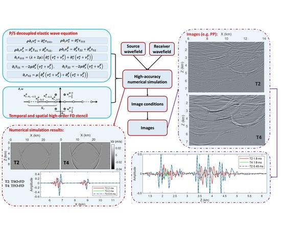
We note that the effect of the temporal dispersion on elastic full-waveform inversion has already been studied [48,49,50], as has acoustic RTM [51]. However, ERTM with a k-space high-order temporal FD method has not been reported. This paper is organized as follows. A quasi-stress–velocity elastic wave equation is derived in the form of P- and S-wave decomposition. Different from the conventional stress–velocity elastic equation, the used equation distinguishes the spatial derivatives related to P- and S-waves, and realizes the decomposition of particle velocity wavefields. Then, the equation is solved by a temporal fourth-order and spatial high-order FD method [52]. The SGFD stencils and the SGFD coefficients are used to propagate waves under the Courant–Friedrichs–Lewy (CFL) stability condition. After obtaining the decoupled source and receiver wavefields through high-precision simulations, the normalized dot-product imaging conditions are used to compute the images, representing a novel ERTM workflow. Finally, the advantages of the proposed ERTM workflow are validated on three synthetic examples and a field data application.

2. Theory and Methods

2.1. Quasi-Stress–Velocity Elastic Equation in the Form of P/S Decomposition

In a two-dimensional heterogeneous isotropic medium, the first-order stress–velocity elastic equation [53], ignoring source terms, is defined as:

$${\partial }_t\mathsf{\phi }-E\mathsf{\phi }=0,$$

(1)

where wavefield $\mathsf{\phi }={\left[\begin{array}{cc}v& \mathsf{\tau }\end{array}\right]}^{\mathrm{T}}$, particle velocity components $v=\left[\begin{array}{cc}{v}_1& v_2\end{array}\right]=\left[\begin{array}{cc}{v}_x& v_z\end{array}\right]$, particle stress components $\mathsf{\tau }=\left[\begin{array}{ccc}{\tau }_{11}& {\tau }_{22}& {\tau }_{12}\end{array}\right]=\left[\begin{array}{ccc}{\tau }_{xx}& {\tau }_{zz}& {\tau }_{xz}\end{array}\right]$, ${\partial }_t(\cdot )$is the first-order temporal differential operator, T is the transpose of a matrix, and matrix operator $E$ describes the interaction between the wavefield and the elastic parameters, is expressed as:

$$E=\left[\begin{array}{ccccc}0& 0& \frac{1}{\rho }{\partial }_x& 0& \frac{1}{\rho }{\partial }_z\\ 0& 0& 0& \frac{1}{\rho }{\partial }_z& \frac{1}{\rho }{\partial }_x\\ \left(\lambda +2\mu \right){\partial }_x& \lambda {\partial }_z& 0& 0& 0\\ \lambda {\partial }_x& \left(\lambda +2\mu \right){\partial }_z& 0& 0& 0\\ \mu {\partial }_z& \mu {\partial }_x& 0& 0& 0\end{array}\right],$$

(2)

where $\rho$ is the density, $\lambda$ and $\mu$ denote the Lamé parameters, and ${\partial }_r(\cdot ) \left(r=x \mathrm{or} z\right)$represents the spatial derivative with respect to $r$.

The P- and S-waves are mixed when numerically simulated using the conventional stress–velocity equation. To effectively figure out the P/S wavefields of particle velocity components for images, we rewrote ${\tau }_{11}$, ${\tau }_{22}$ as ${\tau }_{11}={\tilde{\tau }}_{11}+{\tau }_{111}$, ${\tau }_{22}={\tilde{\tau }}_{22}+{\tau }_{111}$. We used the term, ${\tau }_{111}$ to calculate the derivatives related to the P-waves, and used the remaining terms, ${\tilde{\tau }}_{11}$ and ${\tilde{\tau }}_{22}$, to calculate the derivatives related to the S-waves [52]. As such, the quasi-stress–velocity elastic equation in a P- and S-wave decomposition form is given by:

$${\partial }_t\tilde{\mathsf{\phi }}-\tilde{E}\tilde{\mathsf{\phi }}=0,$$

(3)

where wavefield $\tilde{\mathsf{\phi }}={\left[\begin{array}{cc}\tilde{v}& \tilde{\mathsf{\tau }}\end{array}\right]}^{\mathrm{T}},$ particle velocity components $\tilde{v}=\left[\begin{array}{cccc}{v}_x^{\alpha }& v_x^{\beta }& v_z^{\alpha }& v_z^{\beta }\end{array}\right]$, $v_x=v_x^{\alpha }+v_x^{\beta }$, $v_z=v_z^{\alpha }+v_z^{\beta }$, particle stress components $\tilde{\mathsf{\tau }}=\left[\begin{array}{cccc}{\tau }_{111}& {\tilde{\tau }}_{11}& {\tilde{\tau }}_{22}& {\tau }_{12}\end{array}\right]$, and matrix operator $\tilde{E}$ is given by:

$$\tilde{E}=\left[\begin{array}{cccccccc}0& 0& 0& 0& 1/\rho {\partial }_x^{\alpha }& 0& 0& 0\\ 0& 0& 0& 0& 0& 1/\rho {\partial }_x^{\beta }& 0& 1/\rho {\partial }_z^{\beta }\\ 0& 0& 0& 0& 1/\rho {\partial }_z^{\alpha }& 0& 0& 0\\ 0& 0& 0& 0& 0& 0& 1/\rho {\partial }_z^{\beta }& 1/\rho {\partial }_x^{\beta }\\ \left(\lambda +2\mu \right){\partial }_x^{\alpha }& \left(\lambda +2\mu \right){\partial }_x^{\alpha }& \left(\lambda +2\mu \right){\partial }_z^{\alpha }& \left(\lambda +2\mu \right){\partial }_z^{\alpha }& 0& 0& 0& 0\\ 0& 0& -2\mu {\partial }_z^{\beta }& -2\mu {\partial }_z^{\beta }& 0& 0& 0& 0\\ -2\mu {\partial }_x^{\beta }& -2\mu {\partial }_x^{\beta }& 0& 0& 0& 0& 0& 0\\ \mu {\partial }_z^{\beta }& \mu {\partial }_z^{\beta }& \mu {\partial }_x^{\beta }& \mu {\partial }_x^{\beta }& 0& 0& 0& 0\end{array}\right],$$

(4)

where superscripts $\alpha$ or $\beta$ identify the current term relative to P- or S-wave velocity ($v_{\alpha }$ or $v_{\beta }$), respectively, and $\lambda +2\mu =\rho v_{\alpha }^2$ and $\mu =\rho v_{\beta }^2$. $v_x^{\alpha }$ and $v_z^{\alpha }$ are particle velocity components related to the P-wave velocity, meaning they are only included in the P-wave simulation. Regarding $v_x^{\beta }$ and $v_z^{\beta }$, these are particle velocity components are related to the S-wave simulation. We only decoupled the particle velocity components from the above-decoupled quasi-stress–velocity elastic equation by introducing an extra particle stress component. In addition, the spatial derivatives of the P- and S-waves were different, which allowd the use of different FD stencils in calculating P- and S-wavefields.

2.2. Wavefield Simulation Using A High-Accuracy Finite-Difference Scheme

Conventional wavefield simulation has spatial arbitrary even-order accuracy and temporal second-order accuracy, i.e., (2Nr, 2), and Nr represents half of the FD stencil length. This is because it uses wavefield variables at the “on-axis” ($r$-axis) in calculating the spatial derivatives ${\partial }_r^{\alpha \mathrm{or} \beta }(·)$, $\left(r=x \mathrm{or} z\right)$. Since introducing “off-axis” ($r+1 \mathrm{and} r-1$-axis) values in derivative calculation helps to suppress temporal dispersion, an advanced FD stencil (2Nr, 4) was incorporated to provide ERTM with a good high-accuracy modeling kernel. The stencil used the wavefield variables at the $r$-axis and four off-axis wavefield values to approximate the spatial derivatives. The FD scheme achieved fourth-order accuracy in time using wavefields at one time step to compute those at the next time step. Assuming $\chi =\alpha \mathrm{or} \beta$, and $u$ stands for the one of wavefield variables of particle velocity and stress components, the differential discrete solution of ${\partial }_r^{\chi }(\cdot ) \left(r=x \mathrm{or} z\right)$ in matrix operator $\tilde{E}$ is achieved using the (2Nr, 4) FD stencil [32], expressed as follows:

$${\partial }_r^{\chi }u\approx \frac{1}{h_r}\left\{\begin{array}{c}\sum _{n=1}^{N_r}{c}_{n,0}^{r,\chi }\left(u_{r+n+0.5}^{\varphi }-u_{r-n+0.5}^{\varphi }\right)\\ +c_{1,1}^{r\varphi ,\chi }\left(u_{r+0.5}^{\varphi +1}-u_{r-0.5}^{\varphi +1}+u_{r+0.5}^{\varphi -1}-u_{r-0.5}^{\varphi -1}\right)\end{array}\right\},$$

(5)

where subscripts $r,\varphi \in \left(x, z\right)$, $r\ne \varphi .$ Here, $r$ and $\varphi$ represent coordinate axes that are perpendicular to each other, h_r represents the grid interval along the r-axis. The letter c represents the FD coefficients, where one part is used for on-axis difference computation and the other part is for off-axis computation.

We matched the Fourier response of the FD discretized Laplacian to the P/S-wave velocity-dependent second-order k-space operator, and determined the temporal fourth-order accuracy FD coefficients using the Taylor-series expansion approach [32]. The FD coefficients in Equation (5) are expressed as follows:

$$\{\begin{array}{c}{c}_{1,1}^{r\varphi ,\chi }=\frac{1}{24}{\gamma }_{\varphi ,\chi }^2,\\ c_{n,0}^{r,\chi }=\frac{{\left(-1\right)}^{n+1}}{2n-1}\sum _{m=1,m\ne n}^{N_r}\frac{{\left(2m-1\right)}^2-{\gamma }_{r,\chi }^2}{\left|{\left(2n-1\right)}^2-{\left(2m-1\right)}^2\right|},\left(n=2,3,\cdots ,N_r\right),\\ c_{1,0}^{r,\chi }=1-2c_{1,1}^{r\varphi ,\chi }-\sum _{n=2}^{N_r}\left(2n-1\right)c_{n,0}^{r,\chi },\end{array}$$

(6)

where ${\gamma }_{r,\chi }=\frac{v_{\chi }\mathsf{\Delta }t}{h_r}$, ${\gamma }_{\varphi ,\chi }=\frac{v_{\chi }\mathsf{\Delta }t}{h_{\varphi }}$, and $v_{\chi }$ is the seismic wave velocity of type $\chi$. Here, $h_{\varphi }$ denotes the spatial interval along the direction $\varphi \in \left(x, z\right).$ Moreover, Δ$t$ denotes the time interval. The CFL stability condition for the simulation using the (2Nr, 4) FD stencil follows the rule

$$v_{\chi }\mathsf{\Delta }t\sqrt{\frac{s_{r,\chi }^2}{h_r^2}+\frac{s_{\varphi ,\chi }^2}{h_{\varphi }^2}}\le 1,$$

(7)

where $s_{r,\chi }=\sum _{m=1}^{N_r}\left|c_{m,0}^{r,\chi }\right|-2c_{1,1}^{r\varphi ,\chi },$ $s_{\varphi ,\chi }=\sum _{m=1}^{N_r}\left|c_{m,0}^{\varphi ,\chi }\right|-2c_{1,1}^{\varphi r,\chi },$ $r,\varphi \in \left(x, z\right),$ $r\ne \varphi .$ Smaller $s_{r,\chi }$ (or $s_{\varphi ,\chi }$) allows a larger $\mathsf{\Delta }t$ when compared with ${\stackrel{⁔}{s}}_{r,\chi }=\sum _{m=1}^{N_r}\left|c_{m,0}^{r,\chi }\right|$ (or ${\stackrel{⁔}{s}}_{\varphi ,\chi }=\sum _{m=1}^{N_r}\left|c_{m,0}^{\varphi ,\chi }\right|$) of the traditional (2Nr, 2) FD stencil, indicating a more relaxed CFL stability condition of the (2Nr, 4) FD stencil.

The truncation error is $o\left(\mathsf{\Delta }{t}^4\right)+o\left(h_r^{2N_r}\right)$ for the (2Nr, 4) FD scheme, meaning that such FD simulation can achieve fourth-order temporal and any even-order spatial (2Nr) accuracy. Due to $\chi =\alpha \mathrm{or} \beta$, we could adopt two groups of independent FD coefficients and CFL stability conditions to propagate the separated P- and S-waves, which helped overcome the problem of undersampling of the S-wave and oversampling of the P-wave in simulation.

2.3. Vector-Based ERTM Using High-Precision P/S Wavefields

ERTM uses the following four main steps to image subsurface reflectivities:

(1) Forward modeling of the source wavefield using the quasi-stress–velocity equation solved by the (2Nr, 4) finite-difference method and storage of the wavefield along the domain boundary to save memory;

(2) Reconstruction of the source wavefield via the stored boundary condition in reverse time;

(3) Backward modeling of the receiver wavefield using the quasi-stress–velocity equation solved by the (2Nr, 4) finite-difference method in reverse time;

(4) Application of imaging conditions to source and receiver wavefields during reverse-time propagation.

The vector-based PP- and PS-wave imaging conditions are given by the following modified formula [42]:

$$I^{\alpha \alpha }\left(\mathit{x}\right)=\frac{{\int }_0^{T_{max}}{\mathit{sgn}}^{\alpha \alpha }\left(\mathit{x},t\right)║{\overrightarrow{\mathit{v}}}^{\alpha }\left(\mathit{x},t\right)║║{\overleftarrow{\mathit{v}}}^{\alpha }\left(\mathit{x},t\right)║dt}{{\int }_0^{T_{max}}{\overrightarrow{\mathit{v}}}^{\alpha }{║\left(\mathit{x},t\right)║}^{2}dt},$$

(8)

$$I^{\alpha \beta }\left(\mathit{x}\right)=\frac{{\int }_0^{T_{max}}{\mathit{sgn}}^{\alpha \beta }\left(\mathit{x},t\right)║{\overrightarrow{\mathit{v}}}^{\alpha }\left(\mathit{x},t\right)║║{\overleftarrow{\mathit{v}}}^{\beta }\left(\mathit{x},t\right)║dt}{{\int }_0^{T_{max}}║{\overrightarrow{\mathit{v}}}^{\alpha }{\left(\mathit{x},t\right)║}^{2}dt},$$

(9)

where the decoupled forward wavefields of particle velocity components include ${\overrightarrow{\mathit{v}}}^{\alpha }\left(\mathit{x},t\right)={\left({\overrightarrow{v}}_x^{\alpha },{\overrightarrow{v}}_z^{\alpha }\right)}^{\mathrm{T}}$ and ${\overrightarrow{\mathit{v}}}^{\beta }\left(\mathit{x},t\right)={\left({\overrightarrow{v}}_x^{\beta },{\overrightarrow{v}}_z^{\beta }\right)}^{\mathrm{T}}$, and the backward wavefields of particle velocity components include ${\overleftarrow{\mathit{v}}}^{\alpha }\left(\mathit{x},t\right)={\left({\overleftarrow{v}}_x^{\alpha },{\overleftarrow{v}}_z^{\alpha }\right)}^{\mathrm{T}}$ and ${\overleftarrow{\mathit{v}}}^{\beta }\left(\mathit{x},t\right)={\left({\overleftarrow{v}}_x^{\beta },{\overleftarrow{v}}_z^{\beta }\right)}^{\mathrm{T}}.$ Here, $I^{\alpha \alpha }\left(x\right)$ and $I^{\alpha \beta }\left(x\right)$ represent the imaging for the PP and PS reflectivities, respectively; $T_{max}$ represents the maximum recorded time; and $║·║$ is the absolute value. Finally, ${\mathrm{sgn}}^{\alpha \alpha }$ and ${\mathrm{sgn}}^{\alpha \beta }$ are the signs for the two images, which can be calculated using the following equations:

$${\mathit{sgn}}^{\alpha \alpha }\left(\mathit{x},t\right)=\{\begin{array}{c}+1\hspace{1em}\mathrm{if} {\overrightarrow{v}}^{\alpha }\left(\mathit{x},t\right)\cdot {\overleftarrow{\mathit{v}}}^{\alpha }\left(\mathit{x},t\right)>0,\\ -1\hspace{1em}\mathrm{if} {\overrightarrow{v}}^{\alpha }\left(\mathit{x},t\right)\cdot {\overleftarrow{\mathit{v}}}^{\alpha }\left(\mathit{x},t\right)\le 0,\end{array}$$

(10)

$${\mathit{sgn}}^{\alpha \beta }\left(\mathit{x},t\right)=\{\begin{array}{c}+1\hspace{1em}\mathrm{if} {\overrightarrow{v}}^{\alpha }\left(\mathit{x},t\right)\cdot {\overleftarrow{\mathit{v}}}^{\beta }\left(\mathit{x},t\right)>0,\\ -1\hspace{1em}\mathrm{if} {\overrightarrow{v}}^{\alpha }\left(\mathit{x},t\right)\cdot {\overleftarrow{\mathit{v}}}^{\beta }\left(\mathit{x},t\right)\le 0,\end{array}$$

(11)

where “·” represents the inner-product operator between two vectors. It is noted from the imaging conditions that the sign of the inner-product operation is preserved, while the amplitude is recalculated with the multiplication of the absolute values of the decoupled forward and backward wavefields.

3. Numerical Examples

3.1. Wavefield Simulation and Decomposition

The accuracy and efficiency of the temporal second-order (TSO) and temporal fourth-order (TFO) FD methods were investigated here via numerical simulation. Accordingly, the two-layered model was discretized into 1500 × 500 grid points with a grid interval of 20 m in both directions. A constant density was used in this example. The two-layer P-wave velocities were 3.0 and 4.0 km/s, respectively, while the two-layer S-wave velocities were 1.8 and 2.4 km/s, respectively.

First, the same spatial FD order and time step, i.e., 2Nr = 8 and Δt = 2 ms, respectively, were used for both methods. Figure 1a,b shows snapshots of $v_z=v_z^{\alpha }+v_z^{\beta }$ at 3.35 s using (8, 2) and (8, 4) FD stencils. It was noted that the wavefields from the TSO method suffered from visible temporal dispersion in their wavefronts compared with those from the TFO method. A reference wavefield (Figure 1c) was calculated using the TSO method with Δt = 0.5 ms and 2Nr = 12 to obtain a reference for comparison. We noted from the P- and S-wave profile comparison given in Figure 1d–f that the TFO method with Δt = 2.0 ms agreed well with the reference wavefield, with a root mean square error (RMSE) of 0.0025 m/s. In contrast, the TSO method had a large RMSE of 0.042 m/s. Regarding the efficiency, the 10-source/6-s simulation tests with the TSO and TFO methods took 17.93 and 19.04 s, respectively, on a GPU card named RTX 3090. It could thus be concluded that the TFO-FD scheme had an extra cost of approximately 6.12% compared with the conventional TSO-FD scheme.

Second, the CFL conditions of both methods were taken into consideration. As the TFO method has a more relaxed CFL condition, which benefits efficiency, different time steps were set for the different methods. In particular, Δt = 2.7 ms was set for the TSO method, and Δt = 3.1 ms was set for the TFO method. Note that these time steps were 98.23% and 97.21%, respectively, of the maximum allowed P-wave time step for the TSO and TFO methods, respectively. Figure 2 displays snapshots of v_z at 3.35 s. The RMSEs were 0.051 and 0.0020 m/s, and the 10-source/6-s simulation tests took 13.37 and 12.06 s for the TSO and TFO methods, respectively. It could thus be concluded that relaxing of the CFL condition can improve the efficiency and will seldom decrease the accuracy of the TFO method.

Third, we noted that the TFO method allows for the use of different FD stencils for P- and S-waves, which is key to elastic wave propagation. Following the above study, (4, 4) and (16, 4) FD stencils were used for derivative calculations related to P- and S-waves, respectively. The RMSEs and 10-source/6-s simulation cost of this test were 0.0017 m/s and 12.67 s, respectively. We found that through the decoupled P- and S-wave FD stencils, based on the TFO method, the accuracy could be improved without additional visible computational cost, compared with that of using the same (8, 4) FD stencil.

Since the vector-based imaging condition requires decoupled P- and S-wavefields, the decoupled results are illustrated for this example. Figure 2b shows the original wavefield $v_z=v_z^{\alpha }+v_z^{\beta }$, and Figure 3 shows the decoupled P-wavefield $v_z^{\alpha }$ and S-wavefield $v_z^{\beta }$. We can see that the wavefield was effectively decoupled based on the quasi-stress–velocity equation simulation using the high-order spatial and temporal FD methods.

3.2. Three-Layer Model Reverse-Time Migration

In this section, we demonstrate the effect of temporal dispersion on the imaging results. The three-layer model with velocity and density parameters is shown in Figure 4a. The model had a grid size of 800 × 400 in the$x$ and $z$ directions, respectively, and the grid interval was 20 m. The migration velocities were generated by smoothing the true parameters with a 200 × 200 m window. The 40 shots of observed data were generated using the (8, 2) FD stencil with Δt = 0.5 ms. A Ricker wavelet of 15 Hz was used in this example.

Two sets of migrations were employed using (8, 2) and (8, 4) FD stencils, respectively. The migration results (Figure 4b–e) were obtained with the ERTM using the TSO-FD and the TFO-FD schemes, both with Δt = 2.0 ms. The observed data were resampled to a time step of Δt = 2.0 ms for the migrations. Based on the migration results, we found that these two methods were able to image the layer boundaries. However, in making a profile comparison (Figure 5), we observed that the images from the TSO-FD scheme with Δt = 2.0 ms had waveform distortion compared with the reference solutions from the TSO-FD scheme with Δt = 0.5 ms. In contrast, the TFO-FD scheme results with Δt = 2.0 ms agreed well with the reference solution, demonstrating the high imaging accuracy of ERTM using the TFO-FD scheme.

3.3. Canadian Foothills Model Reverse-Time Migration

After demonstrating the advantages of the proposed ERTM in a layered medium, this method was applied to the more complex Canadian foothills model. The model size was 500 × 834 with a grid spacing of 20 m. The TSO-FD method using a small time-step of Δt = 0.45 ms was chosen to generate 167 shots of observed data. These shots were excited at the locations of vertical 20 m depth and horizontal 100 m intervals. In the subsequent migration process, these shot gathers were also resampled to a time step of Δt = 1.8 ms. Figure 6 displays the migration velocities used in this example. By choosing constant density, the influence of density variation on the imaging results is temporarily ignored.

In migration imaging, the traditional TSO method and the proposed TFO method were first compared using the same time step Δt = 1.8 ms and spatial order 2N_r = 10. Figure 7 and Figure 8 show the migration results of the two methods. For ease of analysis, the TSO method with a smaller time step Δt = 0.45 ms was used to generate reference images, as shown in Figure 9. It can be seen from the images in Figure 7 and Figure 8 that the traditional ERTM with the TSO-FD scheme failed to obtain the high precision P- and S-wave images (Figure 7a,b, respectively). However, the proposed ERTM with the TFO-FD scheme outperformed the TSO-FD (Figure 8a,b), and presented clear fault points and a clean background, and agreed with the reference images (Figure 9a,b) very well. To further compare the results, the P-wave imaging results and the S-wave imaging results at $x$ = 4.0 km, 10.0 km, and 14.0 km were also extracted, as illustrated in Figure 10 and Figure 11, respectively. From these profile comparisons, it was found that conventional ERTM using a second-order temporal accuracy FD scheme introduced visible imaging errors and produced fake reflectors, as especially evidenced in the results depicted in Figure 11a.

3.4. Field Data Application

After demonstrating the advantages of the proposed method on synthetic data, we conducted a land field data application. There were 240 shots approximately evenly distributed with 80 m intervals. Before migrations were carried out, the data were processed by routine industry procedures, such as surface wave reduction and random noise suppression. Figure 12a shows a middle shot gather, and Figure 12b shows its averaged amplitude spectrum with a central frequency of about 25 Hz.

The P-wave migration velocity was established via full-waveform inversion [54], and the S-wave migration velocity was obtained by assuming a constant Poisson’s ratio, and a constant density of 2.0 g/cm³. Figure 13 shows the migration velocity models, which is 1000 × 300 with a grid interval of 20 m. The record time of the observed data was 5 s, and the wavelet involved in the forward simulation was estimated from the seismic data.

We performed three sets of migrations using TSO-FD with Δt = 0.5 ms and Δt = 2.0 ms, and using TFO-FD with Δt = 2.0 ms, respectively. We used a spatial FD order of 2N_r = 10 for all numerical simulations. The migration results of the TSO method using Δt = 0.5 ms were used as a reference in the subsequent comparisons. Figure 14 and Figure 15 depict the final PP- and PS-wave images calculated using the TSO and TFO methods with the same time step of Δt = 2.0 ms. These images show that the PP-wave imaging results (Figure 14a and Figure 15a) have clearer structures and stronger shallow reflectivities than the PS imaging result (Figure 14b and Figure 15b). This phenomenon may be because the S-wave migration velocity is not accurate enough. When focusing on the image comparison between the TSO and TFO methods, we noticed that the results in the rectangular areas related to the proposed TFO method had better event continuity and stronger energy than those of the TSO results.

To further compare, we displayed the zoomed-in parts of Figure 14 and Figure 15 in Figure 16a–d, respectively. Figure 16 proves that the images calculated by the proposed ERTM method are very close to the reference images (Figure 16e,f), both in terms of imaging depth and imaging energy focus. Finally, we extracted the three profiles from the migration results shown in Figure 14 and Figure 15, and used reference solutions to check the accuracy of images further. Figure 17 and Figure 18 display PP- and PS-wave image profiles from locations $x$ = 6.5 km, $x$ = 12.5 km, and $x$ = 18.0 km, respectively. We observed that the results computed by the proposed method were in good agreement with the reference solutions, without the visible changes in reflection locations and waveforms. In contrast, the conventional ERTM resulted in significant changes in imaging locations and waveform energy. In other words, conventional ERTM cannot provide high-precision images for attribute analysis and could mislead the drilling deployment.

In summary, through the above wavefield simulations and synthetic and field data migration experiments, we observed that the time dispersion would lead to travel time changes and waveform distortions, which in turn affects the migration results. The time dispersion effect is manifested in the fact that the depth of the imaging horizon appears deeper in layered media, and the diffracted waves cannot focus at the scattering points of the complex model. However, with the high-precision imaging method proposed in this paper, the above problems can be well resolved, and the imaging results were almost identical to the reference scheme.

4. Discussion

ERTM is a valuable and efficient method for generating high-wavenumber images, which is gradually becoming an important part of our imaging tools. Though some FD numerical simulations with good temporal discrete accuracy have been proposed, few have been applied to improve ERTM quality. This paper presented a complete ERTM workflow based on a temporal and spatial high-order FD accuracy simulation kernel. We only considered the temporal fourth-order FD accuracy because Chen et al. [52] had demonstrated little accuracy improvement from the temporal sixth-order FD method over the fourth order. Therefore, the temporal fourth-order FD method is enough to meet the wavefield simulation need for high accuracy in ERTM, and does not incur much extra computing cost [32].

In wavefield simulations, the FD coefficient calculations associated with the temporal fourth-order precision scheme include velocities, which differs from the traditional temporal second-order accuracy method. Pre-computing the FD coefficients related to the different velocities before the parallel differential computation can save computation time. Meanwhile, velocity rounding in FD coefficient calculations can reduce the number of FD coefficient pairs, which contributes to efficient indexing in FD calculations.

In our normalized vector-based imaging conditions, we should add a small value in the denominator to avoid dividing over zeroes. We also noticed that too small a value would introduce some noise, while too large value would reduce imaging resolution. This situation was even more evident for noisy field data. In fact, the effect of this kind of regularization on imaging results is universal. We suggest that the small value is 10⁻⁵ to 10⁻³ times the maximum value of the wavefield.

Using a small-time step in the wavefield simulation can suppress the effect of time dispersion in the migration, but a small-time step will inevitably increase the computational cost several times. Choosing a migration imaging method that allows the use of large time steps, such as the one proposed in this paper, can significantly improve the efficiency while keeping the accuracy almost unchanged. In addition, for the field data example, we observe that the temporal dispersion shifts the imaging locations and causes out-of-focus energy in some flat layers, rather than the fake reflectors around diffraction points. Possible reasons for this phenomenon are the lack of scattered waves in the recorded data, inaccurate velocities, or the absence of significant scatterers in the subsurface.

This ERTM workflow is a novel one from the perspective of the P/S-wave decoupled equation and its high-accuracy numerical simulation, which can integrate the most current RTM or least-square RTM techniques [55,56] into this computational framework to suppress both temporal and spatial dispersion and improve imaging quality. In addition, modeling including P/S decomposition has potential value for full-waveform inversion [57,58].

5. Conclusions

We have developed a new high-accuracy ERTM for seismic imaging in complex media. The FD schemes with 2Nr-order accuracy in space and fourth-order accuracy in time ensure the high-precision numerical simulation for the ERTM. The proposed ERTM workflow can achieve effective suppression of the temporal dispersion occurring in conventional temporal second-order accuracy FD schemes with a relatively large time step, ensuring accurate image locations and in-focus diffraction waves. Wavefield simulations validate that the used FD schemes can improve the simulation accuracy and efficiency due to the temporal fourth-order accuracy schemes and relaxed CFL conditions. In conventional ERTM tests, travel time changes and waveform distortions in wavefields caused by temporal dispersion mean that the depth of the imaging horizon appears deeper in layered media and the diffracted waves cannot focus at the scattering points of the complex model. The problem can be effectively overcome by our proposed ERTM, as demonstrated in the proposed ERTM tests. Furthermore, the proposed method is applied to field data and the expected results are obtained. The proposed high-accuracy ERTM workflow facilitates the integration of the most advanced imaging or inversion techniques into this computational framework.