Article

Local Scale (3-m) Soil Moisture Mapping Using SMAP and Planet SuperDove

1
Numerical Terradynamic Simulation Group, W.A. Franke College of Forestry and Conservation, The University of Montana, Missoula, MT 59812, USA
2
NASA Goddard Space Flight Center, Greenbelt, MD 20771, USA
3
Department of Civil Engineering, Monash University, Clayton, VIC 3800, Australia
4
Woodwell Climate Research Center, Falmouth, MA 02540, USA
*
Author to whom correspondence should be addressed.
Remote Sens. 2022, 14(15), 3812; https://doi.org/10.3390/rs14153812
Submission received: 29 June 2022 / Revised: 2 August 2022 / Accepted: 6 August 2022 / Published: 7 August 2022
(This article belongs to the Section Remote Sensing in Geology, Geomorphology and Hydrology)

Abstract

:
A capability for mapping meter-level resolution soil moisture with frequent temporal sampling over large regions is essential for quantifying local-scale environmental heterogeneity and eco-hydrologic behavior. However, available surface soil moisture (SSM) products generally involve much coarser grain sizes ranging from 30 m to several 10 s of kilometers. Hence, a new method is proposed to estimate 3-m resolution SSM using a combination of multi-sensor fusion, machine-learning (ML), and Cumulative Distribution Function (CDF) matching approaches. This method established favorable SSM correspondence between 3-m pixels and overlying 9-km grid cells from overlapping Planet SuperDove (PSD) observations and NASA Soil Moisture Active-Passive (SMAP) mission products. The resulting 3-m SSM predictions showed improved accuracy by reducing absolute bias and RMSE by ~0.01 cm3/cm3 over the original SMAP data in relation to in situ soil moisture measurements for the Australian Yanco region while preserving the high sampling frequency (1–3 day global revisit) and sensitivity to surface wetness (R 0.865) from SMAP. Heterogeneous soil moisture distributions varying with vegetation biomass gradients and irrigation regimes were generally captured within a selected study area. Further algorithm refinement and implementation for regional applications will allow for improvement in water resources management, precision agriculture, and disaster forecasts and responses.

Graphical Abstract

1. Introduction

Surface soil moisture (SSM) exerts a fundamental control on land surface hydrological and ecological processes [1,2] and serves as a key environmental input for a variety of scientific studies and applications such as flood and drought monitoring [3,4], wildfire risk assessment [5], and crop yield forecasts [6].
SSM strongly influences soil thermal and dielectric properties, surface reflectance, and vegetation physiology [7]. Both optical-infrared (IR) and microwave remote sensing techniques provide practical approaches for quantifying the spatial distribution and temporal changes of regional SSM through measuring the electromagnetic signatures of the land surface. Optical-IR sensors are well suited for indirectly inferring surface and root zone soil moisture by monitoring the changes of surface thermal properties (e.g., soil temperature, thermal inertia in the case of bare soil) and surface reflectance properties sensitive to vegetation cover and growth, although, the observations may be degraded by cloud cover, atmosphere aerosols, and sub-optimal illumination conditions [7]. Microwave remote sensing provides direct measurements of soil dielectric properties, which are highly sensitive to soil moisture changes [8]. Satellite active and passive microwave sensors are also capable of day-and-night and nearly all-weather observations of Earth’s surface. The microwave penetration ability is superior to optical-IR wavelengths, with lower frequencies suitable for sensing deeper soil layers.
Operational SSM mapping over the globe mainly relies on space-borne microwave radiometers and scatterometers. For example, SSM at ~1-cm depth has been measured routinely using the Advanced Microwave Scanning Radiometer—EOS (AMSR-E) and AMSR-2 sensors since 2002 [9,10]. The AMSR-E/2 X-band SSM products have reasonable accuracy (RMSE < 0.06 cm3/cm3) for sparsely to moderately vegetated conditions with vegetation water content (VWC) less than 1.5 kg/m2 [9,11]. With the launch of L-band microwave sensors, including the ESA Soil Moisture and Ocean Salinity (SMOS) mission [12] and the NASA Soil Moisture Active-Passive (SMAP) mission [2], significant improvements in SSM retrievals have been made in terms of both accuracy (RMSE < 0.04 cm3/cm3 for VWC < 6 kg/m2), and soil sensing depth (~5 cm) [2,13,14]. In addition, the microwave radiometers onboard polar-orbiting satellites provide 1 to 3-day global revisits suitable for monitoring surface wetness dynamics at a level of performance required for hydrological and ecological studies [10,15]. A major constraint of the satellite microwave radiometers or scatterometers is associated with their coarse product spatial resolutions (e.g., AMSR-E/2 25 km; SMAP 9 km and 36 km), which are unable to characterize local scale (e.g., meter-level) heterogeneity in SSM dynamics.
To overcome the limitations in satellite passive microwave observations, a variety of downscaling techniques have been developed to disintegrate radiometer brightness temperature (Tb) or soil moisture estimates into values for finer-scale pixels [16]. The downscaling approaches generally rely on (a) higher-resolution information inferred from Synthetic Aperture Radar (SAR) observations [17,18], optical-IR remote sensing [19,20,21], or land surface model simulations [22]; and (b) cross-scale relationships among the observations, retrievals or simulations [16,23]. For example, SMOS 36-km SSM was downscaled to 1-km resolution using a triangular feature space defined by MODIS land surface temperature and vegetation index data without significant degradation in accuracy [24]. SMAP Tb data was disintegrated into 1-km pixels by exploiting complementary information provided from Sentinel-1 SAR radar backscatter, and the disaggregated Tb was further used for deriving 1-km resolution SSM [25]. Besides the physically-based approaches, machine learning (ML) methods were successfully used to define the non-linear and cross-scale relationships among soil moisture, satellite observations, and geospatial variables [16]. In particular, tree-based regression models were proven effective in combining a variety of predictor variables from satellites, process models, and in situ measurements for enhancing SSM resolution [20,26,27].
Continuous and local-scale (e.g., from 1-m to 100-m resolutions) surface wetness information is essential for characterizing environmental heterogeneity and dynamics [22,28] and improving applications such as irrigation management [20], household-level flood risk assessment [29], and landslide monitoring [30]. Despite previous downscaling efforts, the potential of meter and sub-meter satellite remote sensing has not been fully explored, considering the growing capability of small or micro-satellites for rapid and high-resolution earth observations. Commercial satellite constellations consisting of optical or SAR sensors such as Planet and Capella are now able to provide global daily/sub-daily coverage at meter-level resolutions. Planet observations have been used for delineating fine-scale surface features such as water and ice over small water bodies [31,32]. The high-resolution images are rich in spatial, spectral, and textural information but also involve very large data loads. Relative to traditional computation performed locally, cloud-based platforms such as Google Earth Engine (GEE) enable more efficient access, processing, and analysis of big data archives [33].
Benefiting from recent advances in remote sensing and cloud computation, this study focused on the synergistic use of high-resolution optical and coarse-resolution microwave sensors and exploited ML and Cumulative Distribution Function (CDF) matching approaches to derive daily and local-scale (3-m) SSM. The work is potentially useful for studies and applications needing improved quantification of land surface heterogeneity.

2. Study Region and Data Sets
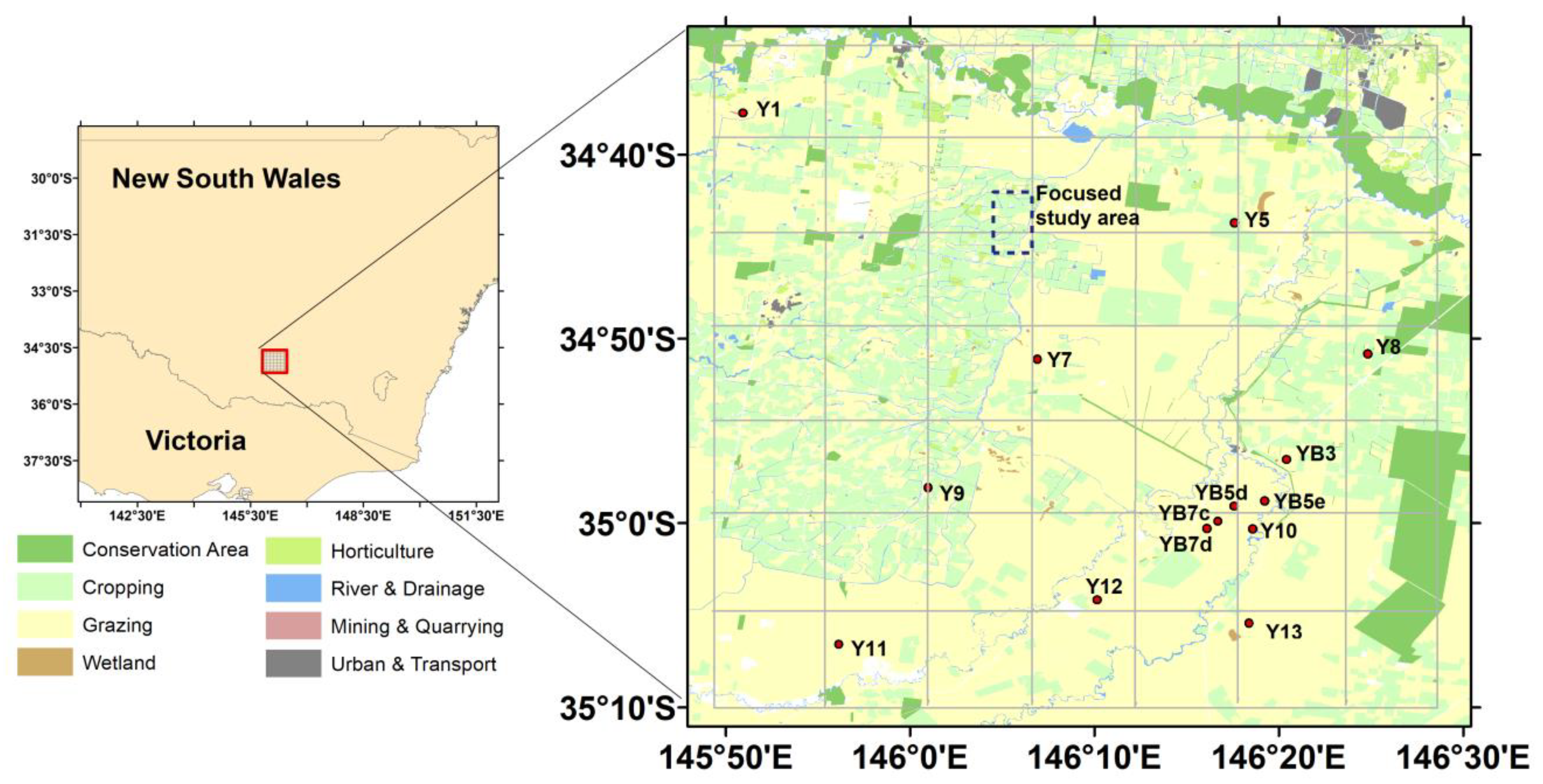
2.1. Study Region

Our study region is a 63 km × 63 km area located in the Yanco area of southern New South Wales, Australia, consisting of 7 by 7 SMAP 9-km grid cells in a global EASE-GRID v2 projection format (Figure 1). The region is characterized by a semi-arid climate, dominated by cropland and grassland, and has been intensely studied in previous field campaigns [19,34,35]. The 9-km grid cells (gray lines in Figure 1) were used to match SMAP SSM and Planet SuperDove (PSD) observations for training a machine learning model. In situ soil moisture stations within the Yanco network are used as a Core Validation Site for assessing SMAP SSM products [14] and were adopted in this study for algorithm evaluation. A focused study area (3 km × 6 km blue rectangle in Figure 1) was selected for examining local-scale SSM distribution patterns, where intensive soil moisture sampling was conducted in March 2021.

2.2. Data Sets

Four major data sets were used for generating and assessing the 3-m SSM results, including (a) long-term in situ soil moisture measurements from the Yanco network, (b) intensive ground measurements using the Hydraprobe Data Acquisition System (HDAS) [36] over the focused study area, (c) PSD 8-band imagery, and (d) SMAP Enhanced L3 Radiometer Global daily 9-km soil moisture (SPL3SMP_E; version 5). In addition, elevation and terrain slope data were obtained from a 5-m Digital Elevation Model (DEM) of Australia [37] to account for terrain effects on soil moisture patterns. Our study focused on an 11-month period from January to December 2021, coinciding with the limited availability of in situ SSM and PSD imagery used for model validation.

2.2.1. Yanco Network

The Yanco soil moisture network is part of the larger Murrumbidgee Soil Moisture Monitoring Network (MSMMN), providing long-term and spatially-distributed SSM measurements [38]. The MSMMN measures surface soil moisture (0–5 cm or 0–8 cm depth) every 20 min, along with soil temperature and rainfall parameters [38]. The 0–5 cm SSM measurement record from January to December 2021 was used for this study and downloaded from the OZNET website (http://www.oznet.org.au/, accessed on 15 January 2022). Among all Yanco stations, only 14 sites (Figure 1) possessing at least 35 data pairs formed by SMAP SSM and clear-sky PSD observations during the study period were selected for evaluating the proposed downscaling approaches.

2.2.2. Intensive Sampling Using HDAS

Intensive sampling of 0–5 cm depth SSM was made using the HDAS at 50 m spacing over the focused study area for a three-week period (8–28 March 2021) during the P-band Radiometer Inferred Soil Moisture 2021 (PRISM-21) campaign (https://www.prism.monash.edu, accessed on 15 January 2022) [39]. Ancillary vegetation and irrigation information was also collected along with soil moisture by the HDAS operators to assist the interpretation of field plot-to-plot soil moisture changes. The intensive sampling data were used to analyze the spatial patterns of the downscaled 3-m SSM results.

2.2.3. PSD 8-Band Imagery

The Planet constellation is currently composed of three generations of satellites, including Dove Classic, Dove-R, and SuperDove, with Equator crossing times between 9:30 and 11:30 [40]. Improved from the first two sensor generations, which capture four-band imagery, SuperDoves allow for eight-band imaging (Coastal Blue, Blue, Green, Green II, Yellow, Red, Red-Edge, and NIR bands) with enhanced image sharpness and quality [40]. Following launches from 2019 to 2022, there are more than 100 SuperDoves on-orbit, which have delivered daily global observations since 2021. In this study, we selected SuperDove imagery obtained with cloud coverage of less than 5% over the study region and period.

2.2.4. SMAP Soil Moisture

The SMAP L-band radiometer has provided twice daily (~6:00 p.m. and a.m. local time) microwave brightness temperature (Tb) observations over the globe since 2015. The SPL3SMP_E was derived from the Tb data spatially interpolated to a finer 9-km global EASE-GRID (v2) resolution using the Backus–Gilbert (BG) technique [41]. The SPL3SMP_E data files record SSM estimates derived using three algorithms, including Single Channel Algorithm (SCA) using V-polarized Tb, SCA using H-polarized Tb, and Dual Channel Algorithm (DCA) [13,14]. As the current baseline, the DCA has shown the best performance among all three SSM retrieval algorithms in comparison with in situ measurements across the globe [42]. The DCA SSM estimates derived from descending (morning pass) SMAP observations were used in this study to pair with PSD morning acquisitions for training an ML model and providing baseline surface wetness information for further downscaling activities. The SMAP data were downloaded through the NSIDC website (https://nsidc.org/data/SPL3SMP_E/versions/5, accessed on 15 January 2022).

2.2.5. Data Processing Using GEE

The GEE is a web-based platform capable of efficient archiving, processing, visualizing, and analysis of multi-petabyte and multi-source data [33]. The high-performance cloud computation capabilities of GEE are suitable for the integrated analysis of large geospatial data sets for environmental applications. For our study, we relied on the GEE Application Programming Interface (API) available in the Google Colab Notebook environment for matching the multi-source data spatially and temporally. Specifically, the SMAP HDF-format data were first converted to GeoTIFF format and then uploaded to GEE as an image collection. Similarly, the PSD images were uploaded to GEE as another image collection. For linking SMAP SSM and PSD spectral observations, SuperDove 3-m pixels were aggregated for each SMAP 9-km grid cell (Figure 1) using GEE by averaging all pixels within the associated grid cell and then matched with SMAP SSM based on date and location. The SMAP and PSD data pairs were then used for training an ML model in the Colab Notebook environment.

3. Methods

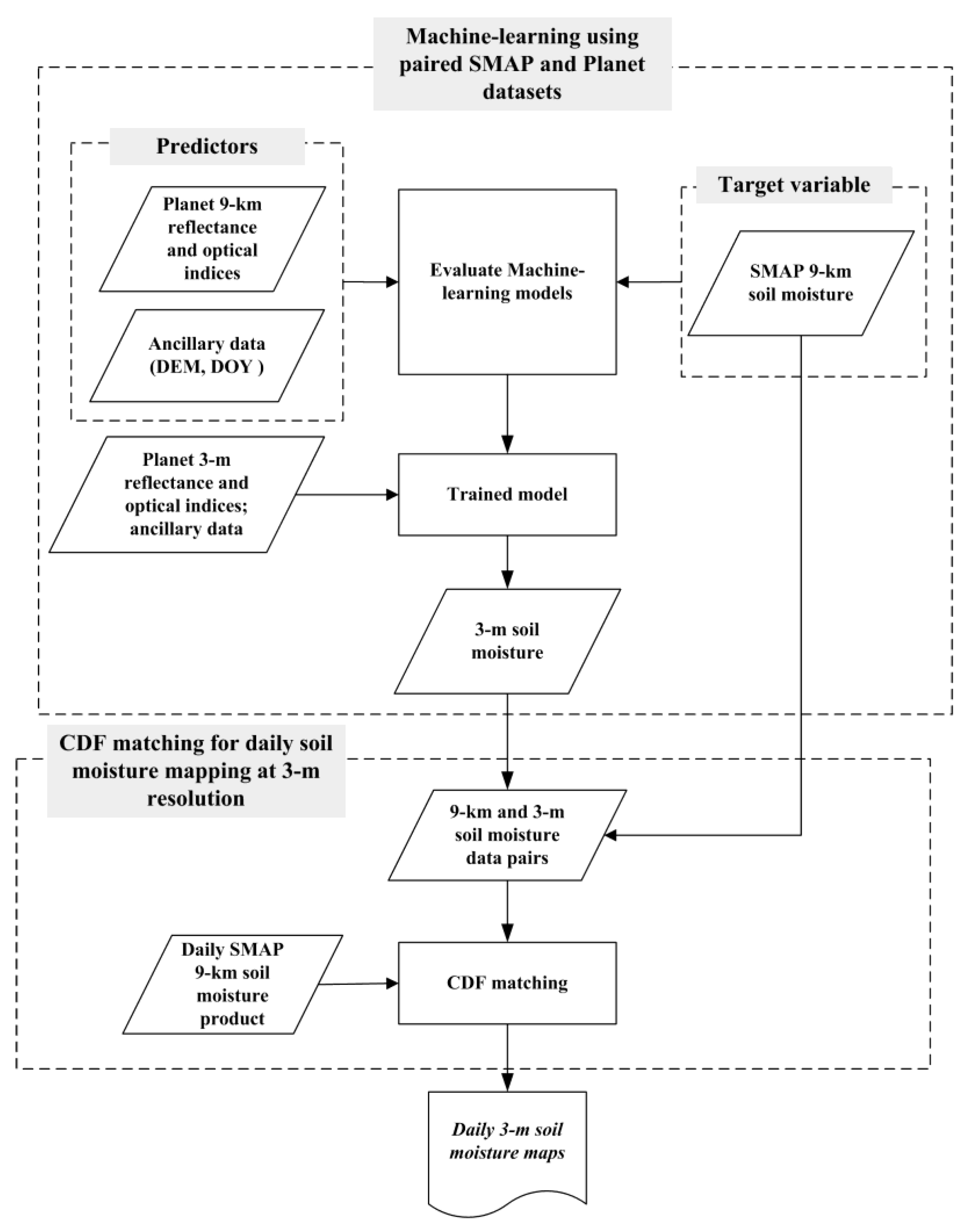
3.1. Approach Overview

This approach (Figure 2) involves a combination of multi-sensor data fusion, ML, and CDF matching for generating daily SSM maps at 3-m spatial resolution. For the ML step, the relationships between predictor variables and the SSM target variable were first derived under SMAP 9-km grid cells. The trained model was then applied to 3-m pixels when both SMAP retrievals and overlapping clear-sky PSD observations were available. Thirty-nine predictor variables were used in this study, including reflectances from all eight PSD spectral bands, normalized reflectance differences calculated from PSD band pairs, terrain information, and the number of each ten-day period in the calendar year (N10DOY) (Table 1).
To overcome the missing PSD data issue caused by cloud and atmospheric constraints, CDF-matching was applied to each 3-m pixel to establish relationships between the SSM target variable and overlying SMAP SSM retrievals and then to apply these empirical models to derive 3-m SSM maps using the SMAP product as the sole model input.
The stepwise algorithm (Figure 2) description is listed below.
(a)
Aggregate all predictor variables for 9-km SMAP grid cells and pair with the corresponding SMAP SSM for the same dates using GEE.
(b)
Perform region-independent cross-validations for model assessment by dividing the SMAP grid cells into seven rows from north to south (Figure 1), selecting data associated with every six rows for model training, and using data from the remaining row for validation. A total of 2100 SMAP and PSD data pairs were used for the assessment.
(c)
Select the best-performing model from the resulting ML algorithms, and apply it to the 3-m PSD data under clear-sky conditions.
(d)
For a given 3-m pixel, perform CDF matching for the SSM estimates of the pixel and the associated SMAP values of the overlying 9-km grid cell, and generate 3-m soil moisture estimates using only the SMAP retrievals as model inputs.

3.2. Machine-Learning Methods

Regression-tree-based ML models and conventional linear regression were used first to establish model relationships between SSM and predictor variables at the SMAP spatial scale (9 km for this study); the resulting trained models were then fed high-resolution inputs to obtain local-scale (3-m) SSM estimates. The regression-tree models have shown high efficiency, good accuracy, and robustness in satellite SSM downscaling studies [16,26] and are generally less affected by data noise and overfitting issues in comparison with other machine learning approaches [43].
The regression-tree methods assessed include Random Forest (RF) [43], Gradient Boosting regression (GBRegrssor) [44] and Light Gradient Boosting Machine regression (LightGBRegressor) [45]. The regression-tree mechanism enables cost-sensitive learning and probability tree estimation [46]. Trees are fit using subsets of explanatory variables and the residual “error” between the predicted and actual values assessed. For the RF approach, a number of trees were built using bootstrap samples, and the final regression results obtained from a forest to provide more accurate and stable predictions than achieved using a single tree [47]. The GBRegressor and LightGBRegressor methods are enhanced versions of tree regression algorithms that adopt gradient boosting, which iteratively constructs the model using the prediction errors from each round [44,45]. In addition to the gradient boosting framework, LightGBRegressor has unique features such as a histogram-based algorithm, exclusive feature bundling, leaf-wise tree growth strategy, histogram difference acceleration, and sequential access gradient methods, which enable high computation efficiency and accuracy [45]. All of the models except LightGBRegressor were implemented using the Python scikit-learn library (https://scikit-learn.org/, accessed on 15 March 2022), with the LightGBRegressor method coded using an independent Python library (https://lightgbm.readthedocs.io, accessed on 15 March 2022). For enabling model inter-comparisons, the same sets of training and validation data were used for each model. The model parameters used for tuning and evaluating the machine learning methods are listed in Table 2. For a given parameter, if two values gave similar performance (e.g., R2 difference less than 0.0025), the smaller value was selected to avoid over-fitting.

3.3. Input Variables Used for ML-Based SSM Prediction

As a key parameter in the soil–plant–atmosphere continuum, soil moisture affects (a) plant water status, composition, structure, and growth; (b) water and energy exchange between the atmosphere and land surface; and (c) the partitioning of rainfall between runoff and infiltration [48,49]. The vertical and horizontal distributions of soil moisture are also regulated by water and energy cycle processes through precipitation, plant canopy interception and evapotranspiration, runoff, and infiltration. Considering the inter-connections among soil moisture and other water and energy cycle components, a number of factors influencing or reflecting the fine-scale soil moisture distributions have been considered in ML-based SSM downscaling studies, including land cover type, vegetation conditions, soil texture, land surface temperature, and topographic information [26]. Different from downscaling studies targeting 30-m to 1000-m SSM mapping, it is challenging to estimate meter-level SSM due to the lack of supporting data at comparable scales. For this study, the feasibility of using PSD 3-m reflectance observations and ancillary terrain and date information (Table 1) for ML-based SSM mapping at local scales was examined. The PSD spectral reflectances and associated indices allow for spectra-based descriptions of surface vegetation and soil conditions at 3-m resolution, the terrain elevation and slope variables govern soil water distributions, and N10DOY is used to account for the general SSM seasonality.

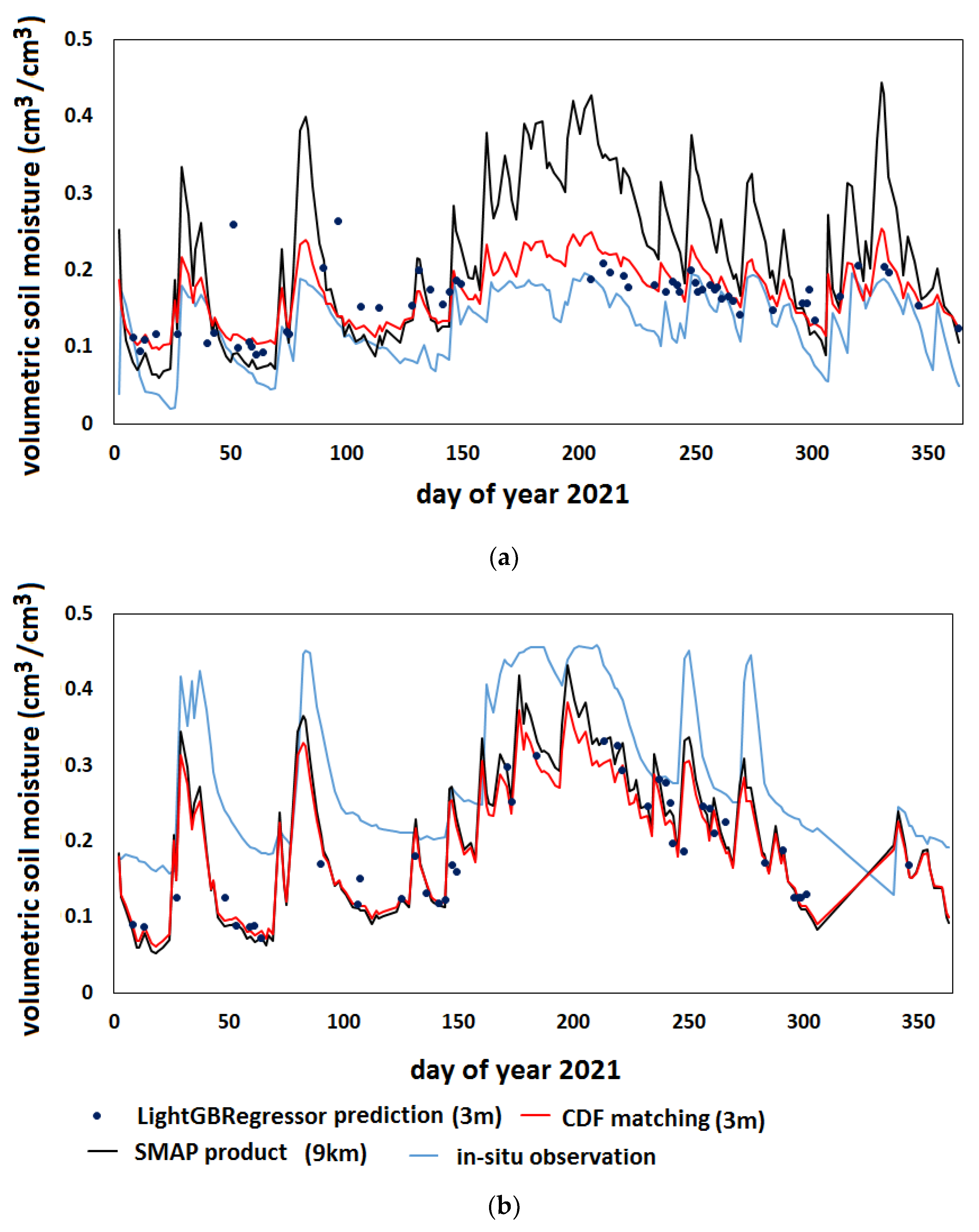
3.4. CDF Matching for Generating Daily SSM Record

CDF matching is a non-linear method widely used for removing biases among soil moisture data sets derived from different approaches, such as satellite passive/active microwave remote sensing, reanalysis, and in situ measurements [50,51,52]. For this study, CDF matching was aimed to relate SSM values obtained from 9-km grid cells and 3-m pixels and generate more temporally continuous SSM data at 3-m resolution. Specifically, SSM data for a given 3-m pixel were first generated using the ML approach and paired with the corresponding SMAP results for the overlying 9-km grid cell. CDF matching was then used to align SMAP SSM data with the 3-m results. The polynomial function for fitting the two data sets was finally applied to the whole SMAP time series to obtain the corresponding SSM estimates for the 3-m pixels without relying on additional PSD observations or ancillary data. Local-scale SSM mapping was thus achieved while preserving the frequent temporal sampling of SMAP.

3.5. Algorithm Assessment

The algorithm assessment consisted of three parts. (a) Examining the performance of the ML models in predicting SSM at 9-km resolution based on the independent validation data (Section 3.1), using the coefficient of determination (R2) and root mean square error (RMSE) calculated between SMAP SSM and the predicted values as performance metrics; (b) quantitative assessment of the ML and CDF matching based SSM downscaling results using the original SMAP 9-km product, the resulting 3-m data sets, and in situ measurements. This assessment involved 14 Yanco sites having at least 30 data pairs of SMAP and ML-predicted SSM available for the CDF calculation. The statistical metrics used for evaluating the performance included R2, RMSE, and absolute bias; (c) a qualitative assessment of the resulting local-scale SSM patterns by comparing the 3-m model predictions with the HDAS intensive SSM sampling results.

4. Results

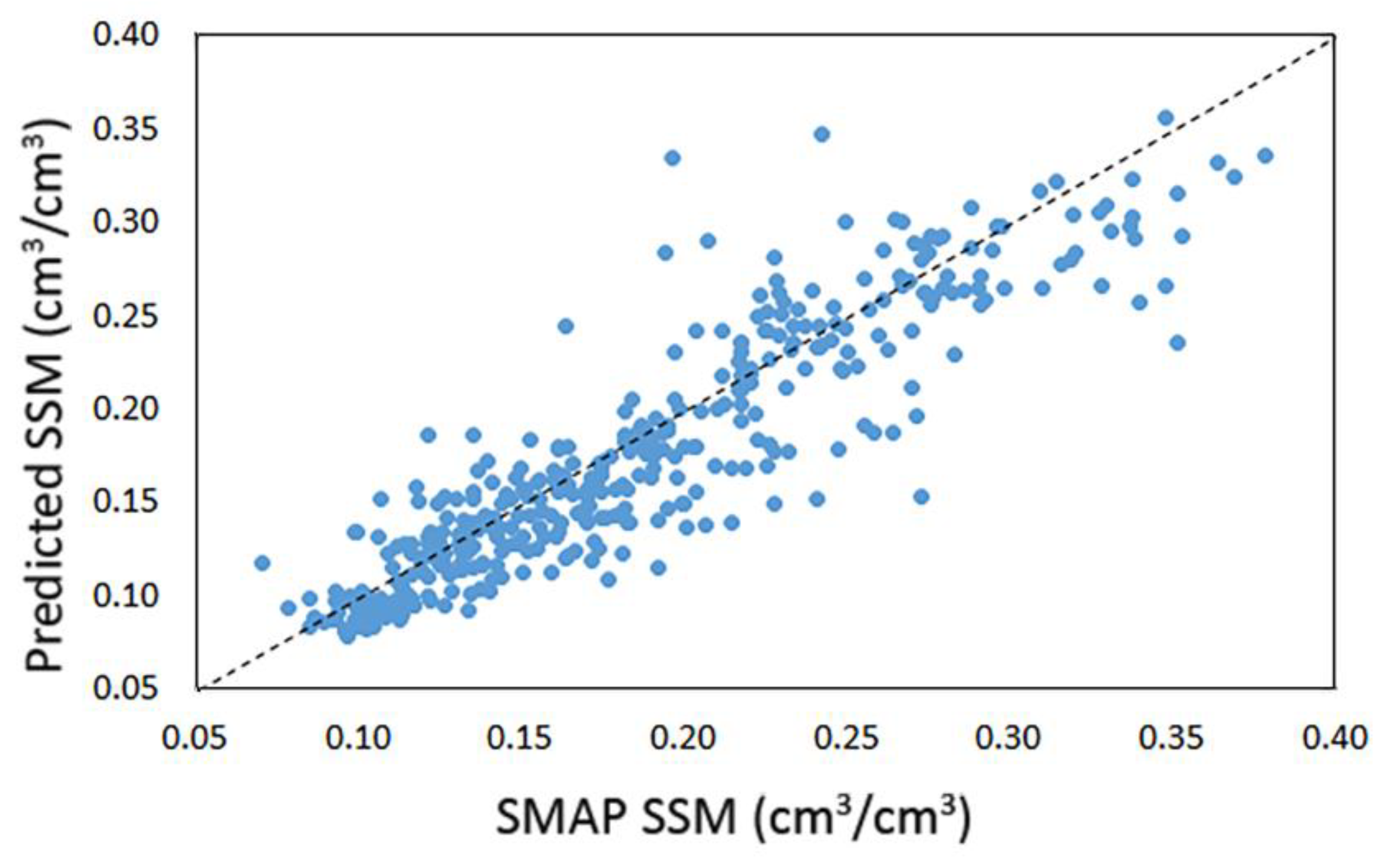
4.1. Assessing the Performance of ML Models in Predicting SSM at 9-km Resolution

In situ soil moisture observations representative of different land cover types, seasons, and geo-locations are scarce and insufficient to support ML model training for global SSM mapping. Therefore, this study trained ML models using the SMAP 9-km SSM product, which has global coverage every 1–3 days. The assessment at the 9-km grid cells showed that the ML models are capable of rebuilding SMAP SSM from finer-grained PSD observations and ancillary information (Table 3). The regression-tree-based methods have similar accuracy when comparing their predictions with the overlying SMAP SSM retrievals (R2 values from 0.846 to 0.857; RMSEs from 0.030 to 0.029 cm3/cm3) while also outperforming the conventional linear regression approach (R2 0.591; RMSE 0.050 cm3/cm3). Among the regression-tree methods, LightGBRegressor is slightly superior to the others in having the highest correlation (R2 0.857) and lowest uncertainty (RMSE 0.029 cm3/cm3) (Figure 3; Table 3). The predictor contribution scores are informative for understanding ML prediction mechanisms and the inter-connections among different input variables and SSM. Among the 39 predictors, the 5 most important variables are N10DOY, near-infrared band reflectance, terrain slope, elevation, and red-edge band reflectance (Table 4). The Normalized Difference Red Edge (NDRE) index, involving red-edge and near-infrared bands, was also an important predictor but with a lower (2.7%) contribution. Low NDRE values typically represent bare soil or stressed vegetation, while higher values indicate healthy vegetation due to NDRE sensitivity to vegetation chlorophyll [53]. Compared to red-edge band reflectance (4.2%) and NDRE (2.7%), the red band and NDVI for measuring vegetation greenness had lower importance, with respective contributions of approximately 1.6% and 1.3%.

4.2. Assessing SSM Predictions at 3-m Resolution

The LightGBRegressor model trained over 9-km grid cells was applied to 3-m pixels for the dates when clear-sky PSD observations were available. After initial predictions over the limited dates, the SSM estimates from LightGBRegressor and SMAP were paired in space and time and then used for CDF matching. The polynomial fit for removing SMAP SSM bias relative to ML-based estimates for a given 3-m pixel was finally applied to the entire SMAP record for generating 3-m SSM time series without the use of additional PSD data.
Comparisons among SMAP 9-km, LightGBRegressor 3-m, and additional CDF matching 3-m results were made for a limited number of dates when all three data sets were available. Among the 14 Yanco sites, CDF matching for the 10 sites led to higher accuracy and lower bias of the 3-m SSM predictions in relation to in situ measurements than the 9-km SMAP SSM retrievals (Table 5). For example, the CDF matching results for Site Y12 dramatically reduced the bias level of SMAP SSM (SMAP absolute bias 0.073 cm3/cm3; CDF matching absolute bias 0.040 cm3/cm3) while removing outliers of the LightGBRegressor predictions (LightGBRegressor RMSE 0.055 cm3/cm3; CDF matching RMSE 0.045 cm3/cm3) (Table 5) and enabling continuous SSM predictions (Figure 4a). For the other four sites, the LightGBRegressor predictions provided no additional value in refining the SMAP SSM time series. For example, the LightGBRegressor SSM results for site Yb5e were very similar to those of SMAP, which did not help to remove SMAP SSM biases in the subsequent CDF matching process (Figure 4b). Overall, the CDF-matching-based SSM results showed a similarly high correlation as the SMAP product (R 0.864) and a low level of absolute bias as the LightGBRegressor estimates (0.043 cm3/cm3), which led to the lowest RMSE (0.062 cm3/cm3) in the comparisons with the in situ SSM measurements (Table 5).
The CDF-matching approach used for the paired LightGBRegressor and SMAP SSM estimates was further applied to the entire SMAP record to generate a continuous 3-m SSM record over the study domain. Among the 14 validation sites, 11 sites showed higher accuracy of the downscaled 3-m SSM data than the original SMAP 9-km results relative to the in situ SSM ground truth measurements (Table 6). Overall, the CDF-matching results lowered the RMSE and absolute bias by ~0.01 cm3/cm3, with RMSE decreasing from 0.081 cm3/cm3 to 0.070 cm3/cm3, while absolute bias declined from 0.052 cm3/cm3 to 0.045 cm3/cm3 (Table 6).

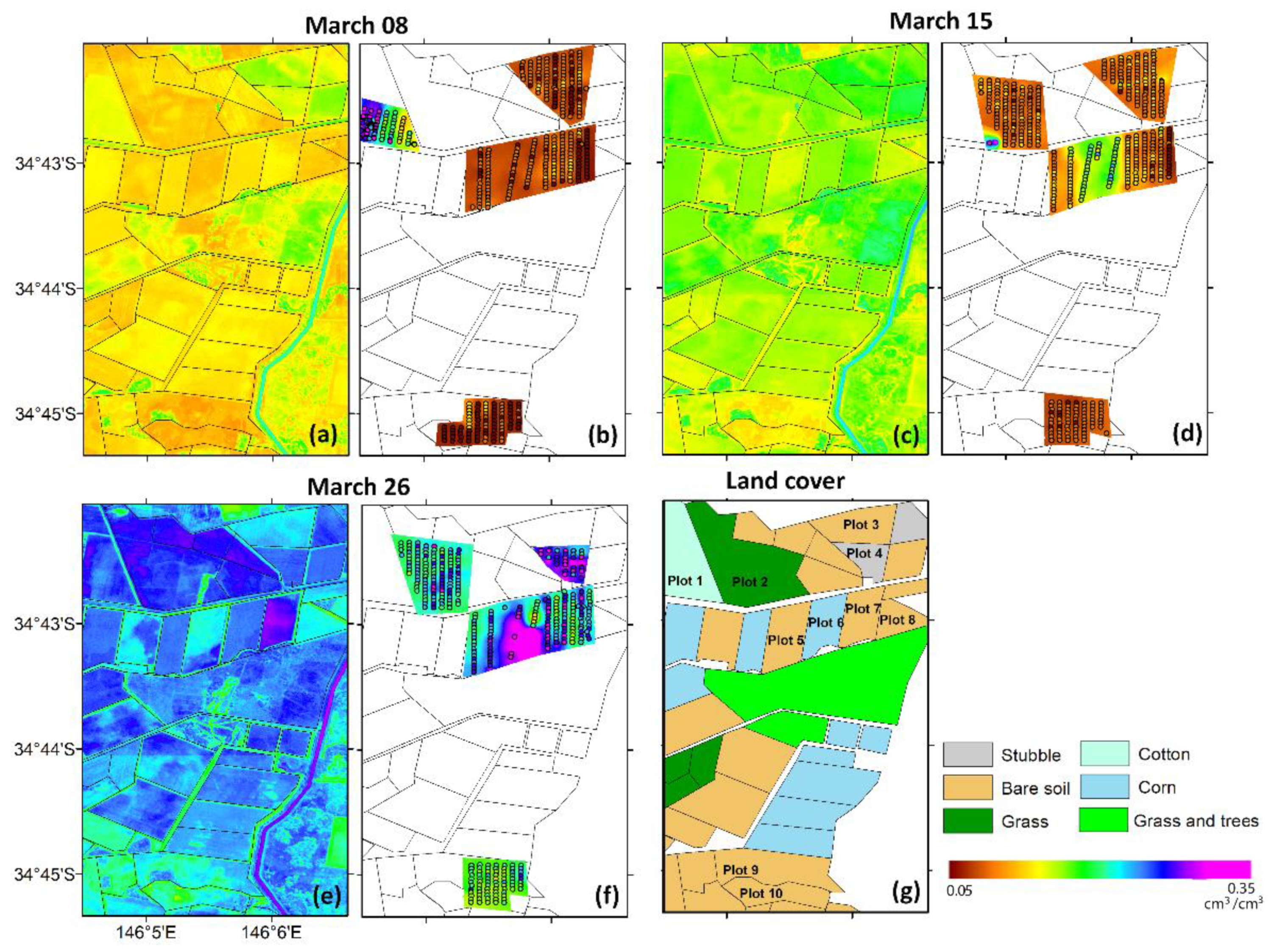
4.3. Evaluating SSM Spatial Distributions at 3-m Resolution

For the focused study area (Section 2.1; Figure 1), spatial distributions of SSM at 3-m resolution derived from the combined ML and CDF matching approach were compared with SSM maps interpolated from HDAS intensive sampling results derived using the Inverse Distance Weighted (IDW) approach for 8, 15, and 26 March 2021 (Figure 5a–f). It is noted that multiple independent SSM measurements were taken using HDAS for each location, and the readings may vary widely in highly heterogeneous areas [39]. The interpolation results were generated based on mean soil moisture values averaged from all readings over a given location. Detailed land cover information (Figure 5g) was also used for the comparisons. The dates were selected for examining the local-scale SSM patterns under distinct surface wetness conditions. In addition, Plots 1 and 6 (Figure 5g) represent managed croplands, which were used to examine irrigation impacts on SSM patterns.
Overall, the downscaled results (Figure 5a–f) captured the contrasting wetness conditions of the three dates as indicated by the HDAS measurements, with high correlation between the two data sets (R 0.81). For 8 March, different from low SSM conditions in most plots, the 3-m results showed wetter soil conditions in the irrigated field (Plot 1), though to a lesser extent than the HDAS readings (Figure 5a,b). Relative to 8 March, larger spatial heterogeneity was found over the fields on March 15, along with similar wetness gradients between non-irrigated (e.g., Plots 8, 9, 10) and irrigated (e.g., Plot 6) fields captured from both the downscaled results and in situ measurements (Figure 5c,d). For 26 March, despite the overall wet conditions, relatively drier soil conditions (Plots 8, 9, and 10) and a noticeable south–north wetness gradient (Plot 5) were apparent in both the downscaled results and HDAS data (Figure 5e,f).
Major inconsistencies between the two data sets were found in Plots 3 and 4 over 8 and 15 March and Plot 2 over 26 March, where wet biases were identified in the downscaled results. By excluding the major outlier plots, the downscaled results have an overall moderate correlation (R 0.45) with the mean HDAS SSM readings (R 0.71 for 8 March, 0.34 for 15 March, and 0.30 for 26 March); and a slightly improved correlation (R 0.54) when comparing with the maximum HDAS readings (R 0.75 for 8 March, 0.45 for 15 March, and 0.41 for 26 March). The HDAS measurements differ from the downscaled results in data acquisition time and spatial representativeness, so the correlation analysis results need to be interpreted cautiously, in particular when high SSM heterogeneity exists and leads to a large difference in HDAS readings at ground sampling locations.
For the areas without HDAS measurements, linear features with lower/higher SSM relative to surrounding pixels were associated with road/drainage systems (Figure 5a,c,e), and higher SSM was found over more densely vegetated areas partially covered by trees (e.g., grass and trees). In comparison, the two 9-km SMAP grid cells (Figure 1) overlying the focused study region were unable to capture a similar level of SSM variability.

5. Discussion

This study proposed a new approach for deriving both high temporal and spatial resolution SSM data using a combination of ML, statistical modeling, and multi-sensor fusion. Of the ML approaches tested, the LightGBRegressor method showed the best performance in estimating SSM using independent and reflectance-based observations over 9-km grid cells (R2 0.857; RMSE 0.029 cm3/cm3). Other regression-tree-based methods are also suitable for this application, given their comparable performance to the LightGBRegressor results (Table 3). These alternative approaches include traditional RF methods widely used for SSM downscaling [20,26] and additional RF refinements using gradient boosting methods. One advantage of this new approach is that the model training does not rely on any in situ observations or measurements from airborne campaigns, which enables the approach to be generally applicable to other regions where high-quality SMAP retrievals are available.
When analyzing the importance of SSM predictor variables, the NDRE was weighted more than NDVI in the ML prediction. Considering the inherent relationships between vegetation growth and soil wetness, NDVI was among the main inputs for downscaling passive microwave SSM [24,26], while this study suggests that vegetation health conditions represented by NDRE are likely related more closely to SSM than the greenness quantified by NDVI. Soil moisture in the Yanco region has clear seasonality with generally drier conditions in the austral summer (DJF) and wetter soil conditions in winter (JJA) [52], which likely led to the relatively high importance of N10DOY in the SSM prediction. In addition, elevation and slope factors are among the most important predictors, which reflect the impacts of topographic control on SSM spatial distributions [26,54]. Despite the high performance of the ML models over the 9-km grid cells, this new approach may still be constrained by the limited spectral information provided by PSD 8-band observations. Richer spectral information, in particular additional thermal band observations used in previous studies [24], may enable further improvements in model performance.
There are two challenges in deriving meter-level SSM using the ML model trained using coarser 9-km grid cell data. One is that the training data sets representing or aggregated for 9-km grid cells may not be comprehensive enough to cover the range of local variability represented from 3-m pixels. The training data were collected from 49 SMAP 9-km grid cells spanning a 12-month period and accounting for a variety of surface soil and vegetation conditions. However, larger study regions and a longer training period would likely enable further algorithm enhancement. Another issue is the relatively sparse temporal coverage of clear-sky PSD observations due to frequent cloud cover causing approximately 80% missing data out of all possible PSD observations during the study period. Although clouds are a well-known constraint in optical remote sensing, this limits the capability of downscaling approaches for generating continuous SSM products needed in many applications, such as irrigation management [20]. In addition, despite the overall lower RMSE and bias of the LightGBRegressor versus 9-km SMAP SSM results relative to the in situ measurements (Table 5), the 3-m ML predictions had relatively lower correlations and more data point outliers (e.g., Figure 4a). To increase the temporal fidelity, the LightGBRegressor results paired with the corresponding SMAP SSM values were fed into the additional CDF matching process. The CDF matching removes outliers in the ML predictions likely caused by noise in PSD reflectance observations under suboptimal atmospheric conditions and, more importantly, for building a continuous SSM time series by accounting for the cross-scale SSM relationships for each 3-m pixel. After applying CDF matching, it was possible to generate SSM time series at 3-m resolution with similarly low RMSE and bias as the LightGBRegressor results while maintaining similar high correlation with in situ observations as the SMAP product.
It is worth noting that the underlying assumptions of our approach are that (a) the SMAP product has high accuracy over the 9-km grid cells, as has been shown for the Yanco region [14], (b) station-based SSM measurements are representative of the overall surface wetness of 3-m pixels, and (c) the ML results can capture the unique soil wetness conditions for a given 3-m pixel. These assumptions held for most of the 14 sites examined (10 sites in Table 5; 11 sites in Table 6), which showed better SSM performance of the downscaled results than the original SMAP product. If the above assumptions are incorrect, no improvement in SSM at fine scales would be expected since the LightGBRegressor results would fail to represent the surface wetness level observed on site (e.g., Figure 4b). The sites without performance enhancement in the downscaled results relative to the SMAP product (e.g., Yb5e, Yb5d, and Yb3; Table 5 and Table 6) are concentrated in a small area with relatively homogeneous soil properties and land use (mainly pasture) [55]. The lack of fine-scale variations in surface properties in this area likely leads to little added contribution to the SSM estimations from high-resolution SuperDove observations. There are no additional measurements within the 3-m pixels for evaluating the spatial representativeness of the in situ SSM measurements; however, differences between the 3-m pixel results and in situ SSM measurements, which may be biased due to site installation and management activities [55], likely contribute to uncertainties in the model validation (Section 4.2; Table 5 and Table 6).
The 3-m SSM distributions over the focused study area were examined under three contrasting wetness conditions. In general, irrigated farms and denser vegetation cover corresponded with higher 3-m SSM levels, while non-irrigated land, bare ground, and roads showed lower wetness. The fine-scale land features with significant SSM spatial variations caused by different irrigation regimes and vegetation cover were generally captured by the downscaled results. A major issue identified is the SSM overestimation relative to the HDAS measurements (e.g., Plots 3 and 4), which was likely caused by high-level retrieval biases as found in other locations (Table 5 and Table 6). In addition, the 3-m SSM estimates for irrigated fields were higher than the surrounding fields but lower than the HDAS measurements. The sub-daily irrigation signals are likely partially missed in the slower changes of vegetation conditions captured by the PDS observations, which led to the underestimation of downscaled SSM.

6. Conclusions

Capabilities for mapping meter-scale soil moisture conditions globally and with high-temporal repeat are essential to local-scale environmental studies and applications. Here, a new method for 3-m SSM mapping was developed by integrating information from satellite passive microwave and high-resolution optical remote sensing through machine-learning and CDF-matching approaches. Compared with the original 9-km SMAP product, the resulting 3-m SSM predictions showed higher accuracy and lower bias in relation to independent soil moisture observations from the Yanco region while preserving the high sensitivity to surface wetness and temporal coverage of SMAP. Complex soil moisture patterns consistent with heterogeneous land cover and vegetation conditions within a focused study area were only captured by the downscaled results. Potential algorithm refinement and implementation for global regions would enable quantification of local-scale land surface heterogeneity and processes for improving the assessment of local environmental changes, disaster risk mitigation, water resources management, and precision agriculture.

Author Contributions

Conceptualization, J.D. and J.S.K.; methodology, J.D. and J.S.K.; validation, J.D. and J.P.W.; formal analysis, J.D., J.S.K., R.B., J.P.W., and J.D.W. writing—original draft preparation, J.D.; writing—review and editing, J.D., J.S.K., R.B., J.P.W., and J.D.W.; visualization, J.D.; supervision, J.S.K.; project administration, J.S.K.; funding acquisition, J.S.K. All authors have read and agreed to the published version of the manuscript.

Funding

This research was funded by the National Aeronautics and Space Administration (NASA), grant number 80NSSC21K1350.

Data Availability Statement

The resulting 3-m SSM data are available from http://files.ntsg.umt.edu/data/SMAP_FW/SSM/ (accessed on 15 June 2022).

Acknowledgments

The Planet SuperDove images were provided by Planet Company with the support of the NASA Commercial Smallsat Data Analysis Program. Data analysis was performed using Google Earth Engine under Colab Notebook environments. SMAP soil moisture data were provided courtesy of the National Snow and Ice Data Center (NSIDC) and downloaded from https://nsidc.org/data/SPL2SMP_E/versions/5 (accessed on 15 January 2022).

Conflicts of Interest

The authors declare no conflict of interest. The funders had no role in the design of the study; in the collection, analyses, or interpretation of data; in the writing of the manuscript; or in the decision to publish the results.

References

  1. Kimball, J.S.; Jones, L.A.; Zhang, K.; Heinsch, F.A.; McDonald, K.C.; Oechel, W.C. A Satellite Approach to Estimate Land–Atmosphere CO2 Exchange for Boreal and Arctic Biomes Using MODIS and AMSR-E. IEEE Trans. Geosci. Remote Sens. 2008, 47, 569–587. [Google Scholar] [CrossRef]
  2. Entekhabi, D.; Njoku, E.G.; O’Neill, P.E.; Kellogg, K.H.; Crow, W.T.; Edelstein, W.N.; Entin, J.K.; Goodman, S.D.; Jackson, T.J.; Johnson, J. The Soil Moisture Active Passive (SMAP) Mission. Proc. IEEE 2010, 98, 704–716. [Google Scholar] [CrossRef]
  3. Bindlish, R.; Crow, W.T.; Jackson, T.J. Role of Passive Microwave Remote Sensing in Improving Flood Forecasts. IEEE Geosci. Remote Sens. Lett. 2008, 6, 112–116. [Google Scholar] [CrossRef]
  4. Du, J.; Kimball, J.S.; Velicogna, I.; Zhao, M.; Jones, L.A.; Watts, J.D.; Kim, Y. Multicomponent Satellite Assessment of Drought Severity in the Contiguous United States from 2002 to 2017 Using AMSR-E and AMSR2. Water Resour. Res. 2019, 55, 5394–5412. [Google Scholar] [CrossRef]
  5. Jia, S.; Kim, S.H.; Nghiem, S.V.; Kafatos, M. Estimating Live Fuel Moisture Using SMAP L-Band Radiometer Soil Moisture for Southern California, USA. Remote Sens. 2019, 11, 1575. [Google Scholar] [CrossRef] [Green Version]
  6. Bolten, J.D.; Crow, W.T.; Zhan, X.; Jackson, T.J.; Reynolds, C.A. Evaluating the Utility of Remotely Sensed Soil Moisture Retrievals for Operational Agricultural Drought Monitoring. IEEE J. Sel. Top. Appl. Earth Obs. Remote Sens. 2009, 3, 57–66. [Google Scholar] [CrossRef] [Green Version]
  7. Zhang, D.; Zhou, G. Estimation of Soil Moisture from Optical and Thermal Remote Sensing: A Review. Sensors 2016, 16, 1308. [Google Scholar] [CrossRef] [Green Version]
  8. Ulaby, F.T.; Moore, R.K.; Fung, A.K. Microwave Remote Sensing: Active and Passive. Volume 3-From Theory to Applications; Artech House: Boston, MA, USA, 1986. [Google Scholar]
  9. Njoku, E.G.; Jackson, T.J.; Lakshmi, V.; Chan, T.K.; Nghiem, S.V. Soil Moisture Retrieval from AMSR-E. IEEE Trans. Geosci. Remote Sens. 2003, 41, 215–229. [Google Scholar] [CrossRef]
  10. Du, J.; Kimball, J.S.; Jones, L.A.; Kim, Y.; Glassy, J.; Watts, J.D. A Global Satellite Environmental Data Record Derived from AMSR-E and AMSR2 Microwave Earth Observations. Earth Syst. Sci. Data 2017, 9, 791–808. [Google Scholar] [CrossRef] [Green Version]
  11. Jackson, T.J.; Cosh, M.H.; Bindlish, R.; Starks, P.J.; Bosch, D.D.; Seyfried, M.; Goodrich, D.C.; Moran, M.S.; Du, J. Validation of Advanced Microwave Scanning Radiometer Soil Moisture Products. IEEE Trans. Geosci. Remote Sens. 2010, 48, 4256–4272. [Google Scholar] [CrossRef]
  12. Kerr, Y.H.; Waldteufel, P.; Wigneron, J.-P.; Martinuzzi, J.; Font, J.; Berger, M. Soil Moisture Retrieval from Space: The Soil Moisture and Ocean Salinity (SMOS) Mission. IEEE Trans. Geosci. Remote Sens. 2001, 39, 1729–1735. [Google Scholar] [CrossRef]
  13. Chan, S.K.; Bindlish, R.; O’Neill, P.; Jackson, T.; Njoku, E.; Dunbar, S.; Chaubell, J.; Piepmeier, J.; Yueh, S.; Entekhabi, D. Development and Assessment of the SMAP Enhanced Passive Soil Moisture Product. Remote Sens. Environ. 2018, 204, 931–941. [Google Scholar] [CrossRef] [Green Version]
  14. Colliander, A.; Jackson, T.J.; Chan, S.K.; O’Neill, P.; Bindlish, R.; Cosh, M.H.; Caldwell, T.; Walker, J.P.; Berg, A.; McNairn, H. An Assessment of the Differences between Spatial Resolution and Grid Size for the SMAP Enhanced Soil Moisture Product over Homogeneous Sites. Remote Sens. Environ. 2018, 207, 65–70. [Google Scholar] [CrossRef]
  15. Kawanishi, T.; Sezai, T.; Ito, Y.; Imaoka, K.; Takeshima, T.; Ishido, Y.; Shibata, A.; Miura, M.; Inahata, H.; Spencer, R.W. The Advanced Microwave Scanning Radiometer for the Earth Observing System (AMSR-E), NASDA’s Contribution to the EOS for Global Energy and Water Cycle Studies. IEEE Trans. Geosci. Remote Sens. 2003, 41, 184–194. [Google Scholar] [CrossRef]
  16. Peng, J.; Loew, A.; Merlin, O.; Verhoest, N.E. A Review of Spatial Downscaling of Satellite Remotely Sensed Soil Moisture. Rev. Geophys. 2017, 55, 341–366. [Google Scholar] [CrossRef]
  17. Das, N.N.; Entekhabi, D.; Dunbar, R.S.; Colliander, A.; Chen, F.; Crow, W.; Jackson, T.J.; Berg, A.; Bosch, D.D.; Caldwell, T. The SMAP Mission Combined Active-Passive Soil Moisture Product at 9 Km and 3 Km Spatial Resolutions. Remote Sens. Environ. 2018, 211, 204–217. [Google Scholar] [CrossRef]
  18. Huang, X.; Ziniti, B.; Cosh, M.H.; Reba, M.; Wang, J.; Torbick, N. Field-Scale Soil Moisture Retrieval Using Palsar-2 Polarimetric Decomposition and Machine Learning. Agronomy 2020, 11, 35. [Google Scholar] [CrossRef]
  19. Merlin, O.; Walker, J.P.; Chehbouni, A.; Kerr, Y. Towards Deterministic Downscaling of SMOS Soil Moisture Using MODIS Derived Soil Evaporative Efficiency. Remote Sens. Environ. 2008, 112, 3935–3946. [Google Scholar] [CrossRef] [Green Version]
  20. Abowarda, A.S.; Bai, L.; Zhang, C.; Long, D.; Li, X.; Huang, Q.; Sun, Z. Generating Surface Soil Moisture at 30 m Spatial Resolution Using Both Data Fusion and Machine Learning toward Better Water Resources Management at the Field Scale. Remote Sens. Environ. 2021, 255, 112301. [Google Scholar] [CrossRef]
  21. Fang, B.; Lakshmi, V.; Cosh, M.; Liu, P.-W.; Bindlish, R.; Jackson, T.J. A Global 1-km Downscaled SMAP Soil Moisture Product Based on Thermal Inertia Theory. Vadose Zone J. 2022, 21, e20182. [Google Scholar] [CrossRef]
  22. Vergopolan, N.; Chaney, N.W.; Beck, H.E.; Pan, M.; Sheffield, J.; Chan, S.; Wood, E.F. Combining Hyper-Resolution Land Surface Modeling with SMAP Brightness Temperatures to Obtain 30-m Soil Moisture Estimates. Remote Sens. Environ. 2020, 242, 111740. [Google Scholar] [CrossRef]
  23. Sabaghy, S.; Walker, J.P.; Renzullo, L.J.; Jackson, T.J. Spatially Enhanced Passive Microwave Derived Soil Moisture: Capabilities and Opportunities. Remote Sens. Environ. 2018, 209, 551–580. [Google Scholar] [CrossRef]
  24. Piles, M.; Camps, A.; Vall-Llossera, M.; Corbella, I.; Panciera, R.; Rudiger, C.; Kerr, Y.H.; Walker, J. Downscaling SMOS-Derived Soil Moisture Using MODIS Visible/Infrared Data. IEEE Trans. Geosci. Remote Sens. 2011, 49, 3156–3166. [Google Scholar] [CrossRef]
  25. Das, N.N.; Entekhabi, D.; Dunbar, R.S.; Chaubell, M.J.; Colliander, A.; Yueh, S.; Jagdhuber, T.; Chen, F.; Crow, W.; O’Neill, P.E. The SMAP and Copernicus Sentinel 1A/B Microwave Active-Passive High Resolution Surface Soil Moisture Product. Remote Sens. Environ. 2019, 233, 111380. [Google Scholar] [CrossRef]
  26. Im, J.; Park, S.; Rhee, J.; Baik, J.; Choi, M. Downscaling of AMSR-E Soil Moisture with MODIS Products Using Machine Learning Approaches. Environ. Earth Sci. 2016, 75, 1120. [Google Scholar] [CrossRef]
  27. Long, D.; Bai, L.; Yan, L.; Zhang, C.; Yang, W.; Lei, H.; Quan, J.; Meng, X.; Shi, C. Generation of Spatially Complete and Daily Continuous Surface Soil Moisture of High Spatial Resolution. Remote Sens. Environ. 2019, 233, 111364. [Google Scholar] [CrossRef]
  28. Du, J.; Watts, J.D.; Jiang, L.; Lu, H.; Cheng, X.; Duguay, C.; Farina, M.; Qiu, Y.; Kim, Y.; Kimball, J.S. Remote Sensing of Environmental Changes in Cold Regions: Methods, Achievements and Challenges. Remote Sens. 2019, 11, 1952. [Google Scholar] [CrossRef] [Green Version]
  29. Du, J.; Kimball, J.S.; Sheffield, J.; Pan, M.; Fisher, C.K.; Beck, H.E.; Wood, E.F. Satellite Flood Inundation Assessment and Forecast Using SMAP and Landsat. IEEE J. Sel. Top. Appl. Earth Obs. Remote Sens. 2021, 14, 6707–6715. [Google Scholar] [CrossRef]
  30. Liao, T.-H.; Kim, S.-B.; Handwerger, A.L.; Fielding, E.J.; Cosh, M.H.; Schulz, W.H. High-Resolution Soil-Moisture Maps Over Landslide Regions in Northern California Grassland Derived From SAR Backscattering Coefficients. IEEE J. Sel. Top. Appl. Earth Obs. Remote Sens. 2021, 14, 4547–4560. [Google Scholar] [CrossRef]
  31. Cooley, S.W.; Smith, L.C.; Stepan, L.; Mascaro, J. Tracking Dynamic Northern Surface Water Changes with High-Frequency Planet CubeSat Imagery. Remote Sens. 2017, 9, 1306. [Google Scholar] [CrossRef] [Green Version]
  32. Kääb, A.; Altena, B.; Mascaro, J. River-Ice and Water Velocities Using the Planet Optical Cubesat Constellation. Hydrol. Earth Syst. Sci. 2019, 23, 4233–4247. [Google Scholar] [CrossRef] [Green Version]
  33. Gorelick, N.; Hancher, M.; Dixon, M.; Ilyushchenko, S.; Thau, D.; Moore, R. Google Earth Engine: Planetary-Scale Geospatial Analysis for Everyone. Remote Sens. Environ. 2017, 202, 18–27. [Google Scholar] [CrossRef]
  34. Panciera, R.; Walker, J.P.; Jackson, T.J.; Gray, D.A.; Tanase, M.A.; Ryu, D.; Monerris, A.; Yardley, H.; Rüdiger, C.; Wu, X. The Soil Moisture Active Passive Experiments (SMAPEx): Toward Soil Moisture Retrieval from the SMAP Mission. IEEE Trans. Geosci. Remote Sens. 2013, 52, 490–507. [Google Scholar] [CrossRef]
  35. Ye, N.; Walker, J.P.; Wu, X.; De Jeu, R.; Gao, Y.; Jackson, T.J.; Jonard, F.; Kim, E.; Merlin, O.; Pauwels, V.R. The Soil Moisture Active Passive Experiments: Validation of the SMAP Products in Australia. IEEE Trans. Geosci. Remote Sens. 2020, 59, 2922–2939. [Google Scholar] [CrossRef]
  36. Merlin, O.; Walker, J.; Panciera, R.; Young, R.; Kalma, J.; Kim, E. Soil Moisture Measurement in Heterogeneous Terrain. In Proceedings of the International Congress on Modelling and Simulation (MODSIM), Christchurch, New Zealand, 10–13 December 2007; pp. 2604–2610. [Google Scholar]
  37. Geoscience Australia. Digital Elevation Model (DEM) of Australia derived from LiDAR 5 Metre Grid; Geoscience Australia: Canberra, Australia, 2015. [Google Scholar]
  38. Smith, A.B.; Walker, J.P.; Western, A.W.; Young, R.I.; Ellett, K.M.; Pipunic, R.C.; Grayson, R.B.; Siriwardena, L.; Chiew, F.H.; Richter, H. The Murrumbidgee Soil Moisture Monitoring Network Data Set. Water Resour. Res. 2012, 48. [Google Scholar] [CrossRef]
  39. Wu, X.; Ye, N.; Walker, J.; Yeo, I.-Y.; Jackson, T.; Kerr, Y.; Kim, E.; McGrath, A. The P-band Radiometer Inferred Soil Moisture Experiment 2021; Workplan; Monash University: Clayton, Australia, 2021. [Google Scholar]
  40. Frazier, A.E.; Hemingway, B.L. A Technical Review of Planet Smallsat Data: Practical Considerations for Processing and Using Planetscope Imagery. Remote Sens. 2021, 13, 3930. [Google Scholar] [CrossRef]
  41. Chaubell, J.; Yueh, S.; Entekhabi, D.; Peng, J. Resolution Enhancement of SMAP Radiometer Data Using the Backus Gilbert Optimum Interpolation Technique. In Proceedings of the 2016 IEEE International Geoscience and Remote Sensing Symposium (IGARSS), Beijing, China, 10–15 July 2016; pp. 284–287. [Google Scholar]
  42. Chaubell, M.J.; Yueh, S.H.; Dunbar, R.S.; Colliander, A.; Chen, F.; Chan, S.K.; Entekhabi, D.; Bindlish, R.; O’Neill, P.E.; Asanuma, J. Improved SMAP Dual-Channel Algorithm for the Retrieval of Soil Moisture. IEEE Trans. Geosci. Remote Sens. 2020, 58, 3894–3905. [Google Scholar] [CrossRef]
  43. Breiman, L.; Friedman, J.H.; Olshen, R.A.; Stone, C.J. Classification and Regression Trees; Routledge: New York, NY, USA, 2017; ISBN 1-315-13947-2. [Google Scholar]
  44. Friedman, J.H. Stochastic Gradient Boosting. Comput. Stat. Data Anal. 2002, 38, 367–378. [Google Scholar] [CrossRef]
  45. Ke, G.; Meng, Q.; Finley, T.; Wang, T.; Chen, W.; Ma, W.; Ye, Q.; Liu, T.-Y. Lightgbm: A Highly Efficient Gradient Boosting Decision Tree. Adv. Neural Inf. Process. Syst. 2017, 30. [Google Scholar]
  46. Steinberg, D. CART: Classification and Regression Trees. In The Top Ten Algorithms in Data Mining; Chapman and Hall/CRC: London, UK, 2009; pp. 193–216. ISBN 0-429-13842-3. [Google Scholar]
  47. Watts, J.D.; Lawrence, R.L. Merging Random Forest Classification with an Object-Oriented Approach for Analysis of Agricultural Lands. Int. Arch. Photogramm. Remote Sens. Spat. Inf. Sci. 2008, 37, 2008. [Google Scholar]
  48. Aubert, D.; Loumagne, C.; Oudin, L. Sequential Assimilation of Soil Moisture and Streamflow Data in a Conceptual Rainfall–Runoff Model. J. Hydrol. 2003, 280, 145–161. [Google Scholar] [CrossRef]
  49. Wang, C.; Fu, B.; Zhang, L.; Xu, Z. Soil Moisture–Plant Interactions: An Ecohydrological Review. J. Soils Sediments 2019, 19, 1–9. [Google Scholar] [CrossRef]
  50. Reichle, R.H.; Koster, R.D. Bias Reduction in Short Records of Satellite Soil Moisture. Geophys. Res. Lett. 2004, 31. [Google Scholar] [CrossRef] [Green Version]
  51. Brocca, L.; Hasenauer, S.; Lacava, T.; Melone, F.; Moramarco, T.; Wagner, W.; Dorigo, W.; Matgen, P.; Martínez-Fernández, J.; Llorens, P. Soil Moisture Estimation through ASCAT and AMSR-E Sensors: An Intercomparison and Validation Study across Europe. Remote Sens. Environ. 2011, 115, 3390–3408. [Google Scholar] [CrossRef]
  52. Su, C.-H.; Ryu, D.; Young, R.I.; Western, A.W.; Wagner, W. Inter-Comparison of Microwave Satellite Soil Moisture Retrievals over the Murrumbidgee Basin, Southeast Australia. Remote Sens. Environ. 2013, 134, 1–11. [Google Scholar] [CrossRef]
  53. Barnes, E.M.; Clarke, T.R.; Richards, S.E.; Colaizzi, P.D.; Haberland, J.; Kostrzewski, M.; Waller, P.; Choi, C.; Riley, E.; Thompson, T. Coincident Detection of Crop Water Stress, Nitrogen Status and Canopy Density Using Ground Based Multispectral Data. In Proceedings of the Fifth International Conference on Precision Agriculture, Bloomington, MN, USA, 16–19 July 2000; Volume 1619, p. 6. [Google Scholar]
  54. Wilson, D.J.; Western, A.W.; Grayson, R.B. A Terrain and Data-Based Method for Generating the Spatial Distribution of Soil Moisture. Adv. Water Resour. 2005, 28, 43–54. [Google Scholar] [CrossRef]
  55. Yee, M.S.; Walker, J.P.; Monerris, A.; Rüdiger, C.; Jackson, T.J. On the Identification of Representative in Situ Soil Moisture Monitoring Stations for the Validation of SMAP Soil Moisture Products in Australia. J. Hydrol. 2016, 537, 367–381. [Google Scholar] [CrossRef]
Figure 1. Location of the study region (red rectangle) consisting of 7 by 7 SMAP 9-km grid cells (gray lines) used for preparing spatially and temporally matched data sets for machine learning, Yanco soil moisture network (stations marked by red circles with names labeled) used for assessing the accuracy of downscaled SSM, and a focused study area (dark blue dash lines) with intensive soil moisture sampling for examining local-scale SSM distribution patterns.
Remotesensing 14 03812 g001
Figure 2. Algorithm flow chart illustrating the proposed downscaling approach for generating 3-m SSM maps based on multi-sensor data fusion, ML, and CDF matching techniques.
Remotesensing 14 03812 g002
Figure 3. Comparison between LightGBRegressor predictions and SMAP SSM at 9-km grid cells (R2 0.857; RMSE 0.029 cm3/cm3).
Remotesensing 14 03812 g003
Figure 4. SSM comparisons among 9-km SMAP product, in situ measurements, and respective 3-m estimates derived using LightGBRegressor and CDF matching for sites Y12 (a) and Yb5e (b).
Remotesensing 14 03812 g004
Figure 5. The downscaled (3-m) SSM patterns derived using the combined ML and CDF-matching approach (a,c,e) and interpolated SSM maps generated from intensive HDAS ground measurement sites (dots) (b,d,f) over the focused study area for 8 March 2021 (a,b), 15 March 2021 (c,d), and 26 March 2021 (e,f); field plots with HDAS measurements are labeled on the land cover map for the same area (g).
Remotesensing 14 03812 g005
Table 1. Summary of the 39 predictor variables used for ML-based SSM prediction.
Predictor NameDescriptionNumber of Predictors
R _ B a n d k Reflectance of PSD band k (k = 1 to 8)8
I n d e x _ B a n d i j Normalized reflectance difference between band i and j28
e l e v a t i o n N/A1
s l o p e N/A1
N 10 D O Y The number of each 10-day period in a year1
Table 2. Summary of model parameters used in evaluating machine-learning methods.
MethodParameterFromToStepOther OptionsSelected
LightGBRegressormax_depth5305 20
n_estimators2012020 120
num_leaves2012020 60
Random forestmax_depth5305 20
n_estimators2012020 100
max_features0.50.90.2‘auto’, ‘log2’, ‘sqrt’0.9
GradientBoostingmax_depth5305 30
n_estimators2012020 60
max_features0.50.90.2‘auto’, ‘log2’, ‘sqrt’0.7
Table 3. Summary of model performance in predicting SSM at 9-km grid cells, with bold numbers denoting the best values.
MethodR2RMSE (cm3/cm3)
LightGBRegressor0.8570.029
Random forest0.8460.030
GradientBoosting0.8560.029
Linear0.5910.050
Table 4. Summary of the contribution scores for the five most important predictors.
PredictorScore
N10DOY7.9%
Near-infrared band reflectance5.9%
Slope4.5%
Elevation4.3%
Red-edge band reflectance4.2%
Table 5. Summary of the SSM comparisons among SMAP 9-km, LightGBRegressor 3-m, and additional CDF matching 3-m results for the dates when all three data sets were available. Bold numbers denote the best model performance at each site.
SiteSMAPLGBMRCDFSMAPLGBMRCDFSMAPLGBMRCDFNumber
RMSE (cm3/cm3)Absolute Bias (cm3/cm3)Correlation
Y80.0410.0400.0300.0090.0050.0050.9020.8410.90641
Yb5e0.0950.1020.0990.0840.0910.0910.8630.8240.86041
Yb5d0.0790.0890.0810.0700.0750.0750.9010.7500.89842
Yb7c0.0730.0640.0610.0630.0500.0500.9060.8680.90644
Yb7d0.0480.0400.0330.0240.0100.0100.8880.8320.88845
Yb30.0640.1080.1040.0360.0750.0750.8490.7070.83444
Y100.0440.0490.0490.0030.0180.0180.9260.9210.92348
Y70.0470.0480.0430.0330.0280.0280.9150.8720.91448
Y10.0970.0770.0750.0860.0660.0660.7600.6700.76355
Y50.0960.0860.0790.0820.0660.0660.7030.5340.70352
Y130.0800.0600.0490.0290.0090.0090.8300.6710.83453
Y90.0660.0740.0610.0480.0420.0420.9240.8320.92454
Y110.0660.0750.0600.0360.0240.0240.8770.7650.87758
Y120.0960.0550.0450.0730.0400.0400.8620.5900.87358
Allsites0.0710.0690.0620.0480.0430.0430.8650.7630.864683
Table 6. Summary of the comparisons among SMAP and CDF matching SSM results over the 12-month study period, with bold numbers denoting the best performance at each in situ validation site.
SiteSMAPCDF_MatchingSMAPCDF_MatchingNumber
RMSE (cm3/cm3)Absolute Bias (cm3/cm3)
Y80.0490.0390.0040.005164
Yb5e0.1000.1070.0860.095163
Yb5d0.0830.0820.0710.071164
Yb7c0.0770.0680.0570.046160
Yb7d0.0640.0440.0370.017163
Yb30.0830.1170.0400.086162
Y100.0570.0620.0070.021178
Y70.0630.0550.0410.035178
Y10.1130.0870.0970.075178
Y50.1070.0850.0910.068178
Y130.0910.0550.0450.019178
Y90.0740.0700.0430.036178
Y110.0660.0620.0260.013178
Y120.1110.0490.0860.040178
Allsites0.0810.0700.0520.0452400
Publisher’s Note: MDPI stays neutral with regard to jurisdictional claims in published maps and institutional affiliations.

