Estimating Large-Scale Interannual Dynamic Impervious Surface Percentages Based on Regional Divisions

Abstract

Impervious surface information is an important indicator to describe urban development and environmental changes. The substantial increase in impervious surface area will have a significant impact on the regional landscape and environment. Therefore, the timely and accurate acquisition of large-scale impervious surface percentage (LISP) is of great significance for urban management and ecological assessment. However, previous LISP estimation methods often ignored the impact of regional geographic environment and climate differences on remote sensing information, resulting in low overall accuracy and obvious regional differences in the estimated results. Thus, in this study, based on the time-series characteristics of multi-temporal remote sensing images combined with the information on geographical environment and climate heterogeneity, a method of time-series remote sensing image fusion and LISP estimation based on regional divisions was proposed. Firstly, the entire region was divided into several regions according to the spatial differences of Köppen–Geiger climate data and MODIS NDVI time-series data. Subsequently, adaptive time-series image fusion methods and remote sensing feature construction methods were proposed for different regions. Finally, the proposed method was used to estimate the percentage of impervious surfaces in other years in Asia. The results indicate that the overall R² of each region is better than 0.82, and the estimation models have a good ability to transfer across time and can directly estimate the impervious surface percentage in other years without using additional samples. In addition, compared with other existing impervious surface products, the proposed method has higher overall estimation accuracy and regional consistency.

1. Introduction

Impervious surfaces are land cover composed of structural materials that hinder the natural penetration of water into the soil including building roofs, asphalt pavements, and hardened grounds [1]. Within the city, impervious surfaces are land cover other than vegetation and bare land. Relevant studies show that the continuous expansion of impervious surface areas has caused social, ecological, and environmental problems such as the heat island effect and traffic jams [2]. At the same time, impervious surface information is also an essential factor and indicator to reflect urban distribution patterns, regional expansion intensity, suitable living environments, and urbanization levels [3]. In addition, large, vegetated areas are converted into impervious areas resulting in a reduction in urban green space. Therefore, these are also the primary data for studying urban flood disasters, biodiversity loss, and other ecological issues [4,5]. At present, the rapid expansion of global cities has brought more comprehensive challenges to regional, national, and global development [6]. Compared with other regions, Asia is in a period of rapid urban population accumulation and accelerated urbanization, and the impervious surfaces are expanding rapidly. Therefore, impervious surface mapping for the Asian region can provide more real-time and accurate basic data for studying urban expansion patterns, climate change, and sustainable development.

In the past two decades, remote sensing images of various spatial resolutions have been used to extract impervious surface information [7]. For high spatial resolution images (≤10 m), object-oriented classification methods are usually used to extract the impervious surfaces [8]. For example, Sebari et al. proposed a fuzzy-object-based analysis method for extracting impervious surface information from IKONOS [9,10]. These methods can comprehensively integrate geometric, textural, spectral, and contextual information, improving spatial resolution and classification accuracy. However, due to the high cost and complex processing, large-scale impervious surface extraction still has challenges. Benefiting from good data availability, researchers tend to use medium-resolution images (10–100 m) [11,12]. The spectral mixture analysis method was proposed for impervious surface inversion using Landsat [13]. However, this method is limited by the choice of pure end members and the complexity of the model, which increases the difficulty of extracting large-scale impervious surface information. Therefore, more methods are used to extract impervious surface information directly by using medium spatial resolution images for classification [14,15,16,17]. For example, Liu et al. made a global impervious surface product based on random forests using Landsat-8 and Sentinel-1 [18] images. Chen et al. proposed a pixel-object-knowledge-based method based on Landsat [19]. However, classification-based methods usually require a classifier supported by training samples. In large-scale information extraction, there are also problems such as unbalanced sample selection and poor generalization ability of the classifier, resulting in large regional differences in classification accuracy and low overall accuracy. Moreover, medium and high spatial resolution sensors usually have a low temporal resolution, which results in the spatial–temporal discontinuity of remote sensing data, further limiting large-scale impervious surface information extraction [20,21,22]. Therefore, it is necessary to comprehensively utilize multi-source and multi-temporal data based on medium and high-resolution images. This greatly increases the difficulty of data preprocessing and model building.

In contrast, coarse spatial resolution data (≥100 m) have been widely used for large-scale information extraction, including impervious surface percentage estimation, due to its higher temporal resolution and spatial coverage. Researchers have used simple and fast index features to distinguish impervious and pervious surface information [23]. However, coarse spatial resolution image pixels are usually dominated by mixed pixels, and the simple threshold method cannot accurately reflect the actual situation. Therefore, based on the basic assumption of mixed pixels, there are more studies that tend to establish the relationship between the impervious surface percentage and remote sensing features through linear or nonlinear regression models [24]. For instance, Guo et al. combined multi-temporal MODIS NDVI and VIIRS DNB data to estimate impervious surface percentage in China through linear regression [25]. Lu et al. fused the time-series MODIS NDVI and DMSP/OLS data to establish a stepwise regression model to predict the impervious surface percentage [26]. This method is simple to operate and has a great predictive effect. Effective feature variables and reasonable regression models are conducive to the rapid realization of large-scale impervious surface percentage inversion [27]. With the release of nighttime light (NTL) remote sensing data, many works began to focus on impervious surface information extraction based on the nighttime light index [28,29]. Among these studies, NTL combined other data to build new indexes such as VANUI (Vegetation-Adjusted NTL Urban Index) and TVANUI (Temperature- and Vegetation-Adjusted NTL Urban Index) [30,31]. Generally, coarse spatial resolution images have better temporal and spatial continuity, providing a reliable data source in large regions. However, with the expansion of the mapping region, impervious surface extraction will be affected by regional land surface differences. In addition, due to regional climates, there are also obvious spatial differences in remote sensing information. For nighttime light data, some issues, such as data oversaturation and unbalanced regional development, directly affect their ability to describe the impervious surface information. Therefore, it remains a challenge to use coarse spatial resolution images to accurately estimate the large-scale impervious surface percentage [32,33].

Spatiotemporal heterogeneity often affects the accuracy of the extraction of large-scale impervious surface information. For temporal sequences, the same object shows obvious differences in images from different periods, and the impervious surface extraction is different in different seasons [34,35]. For example, in the northern summer or vegetation growing season, the spectral difference between the vegetation and impervious surface is large, and the extraction results are better than in other seasons. Therefore, applying multi-temporal data requires consideration of the effects of the temporal differences. In terms of spatial scale, small-scale regional extraction usually does not need to consider the spatial differences [36]. However, for large-scale information extraction affected by differences in terrain and natural ecosystems, the spatial and spectral characteristics of ground objects in remote sensing images show significant differences, which seriously restricts the extraction accuracy. Therefore, researchers have considered a regional division strategy to address the spatial inconsistencies. Gong et al. divided the study area into geographical grids and extracted impervious surfaces for each grid to reduce the spatial differences [37]. However, the grid size is usually set based on the researcher’s experience. In addition, the method needs to provide accurate and effective training data for each grid [19,38]. To balance the data volume and efficiency, Zhang et al. extracted the global impervious surface based on the local adaptive scheme of the grid and adjacent grid [18]. However, the inevitable differences in surface cover form different distribution patterns of impervious surfaces, which affect the extraction accuracy such as areas with sparse vegetation and areas with abundant vegetation. Considering the regional landscape differences, Gong et al. used the global biome distribution to divide the world into arid and non-arid regions based on grids [39]. Huang et al. divided the world into 1221 hexagons, used different DEM data to adapt to the elevation and slope features in different latitudes, and considered adding light features to suppress misclassification in arid regions [40]. Sun et al. improved impervious surface extraction performance by using finer-scale global biome maps in arid and semi-arid regions [41]. However, the differentiation between arid and non-arid regions does not express global landscape differences adequately [42]. A richer regional division strategy is needed to adapt to the extraction of impervious surface information in different regions. To this end, GlobeCover2009 considered the ecological landscape and regional climate change factors and divided the world into 22 ecological regions [43]. Furthermore, Schneider et al. proposed a global urban ecoregion stratification scheme combining global climate characteristics and thematic data [44]. Through this scheme, the NUACI (Normalized Urban Areas Composite Index) obtained the threshold for each ecological region [45]. Those previous studies demonstrated that the regional divisions effectively overcome the impact of spatial heterogeneity of climate and ecology on a large scale. However, most of the proposed division principles are based on regular shapes such as grids and hexagons, ignoring the irregularity of the real boundaries, which significantly increases the sample requirements and operating time based on numerous subregions. In addition, although the combination of landscape patterns and ecological elements improves the pertinence of regional divisions, this process does not consider the temporal and spatial differences of the data itself, which affects the stability of regional information extraction.

Above all, remote sensing data with good spatiotemporal continuity, such as MODIS and NTL, have obvious advantages in estimating the large-scale impervious surface percentage. However, in large-scale regions where land cover exhibits significant spatial differences and seasonally inconsistent dynamics, obtaining accurate and balanced estimates remains a challenge. To this end, this study is motivated by solving the spatiotemporal inconsistencies in the estimation of large-scale impervious surface percentages, and attempts to combine regional climate classification information with the time-series features of remote sensing images to construct a more reasonable regional division method to overcome the influence of regional differences. Based on ensuring the differences in the landscape, a regional division strategy was constructed to realize the rational optimization of the spatial distribution and reduce the regional redundancies. At the same time, an adaptive selection and feature construction model of regional remote sensing image time series is developed to achieve more stable impervious surface features for different regions. Finally, the large-scale impervious surface percentage estimation is realized based on the construction of different regional features and feature set combinations.

2. Materials and Methods

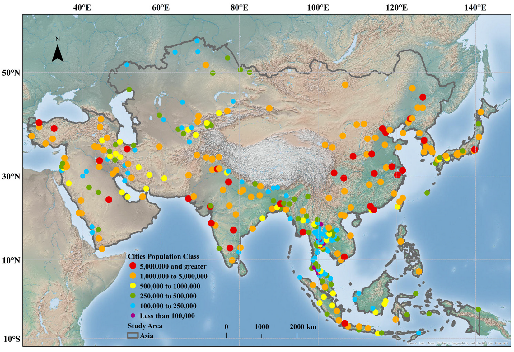
2.1. Study Area and Data Set

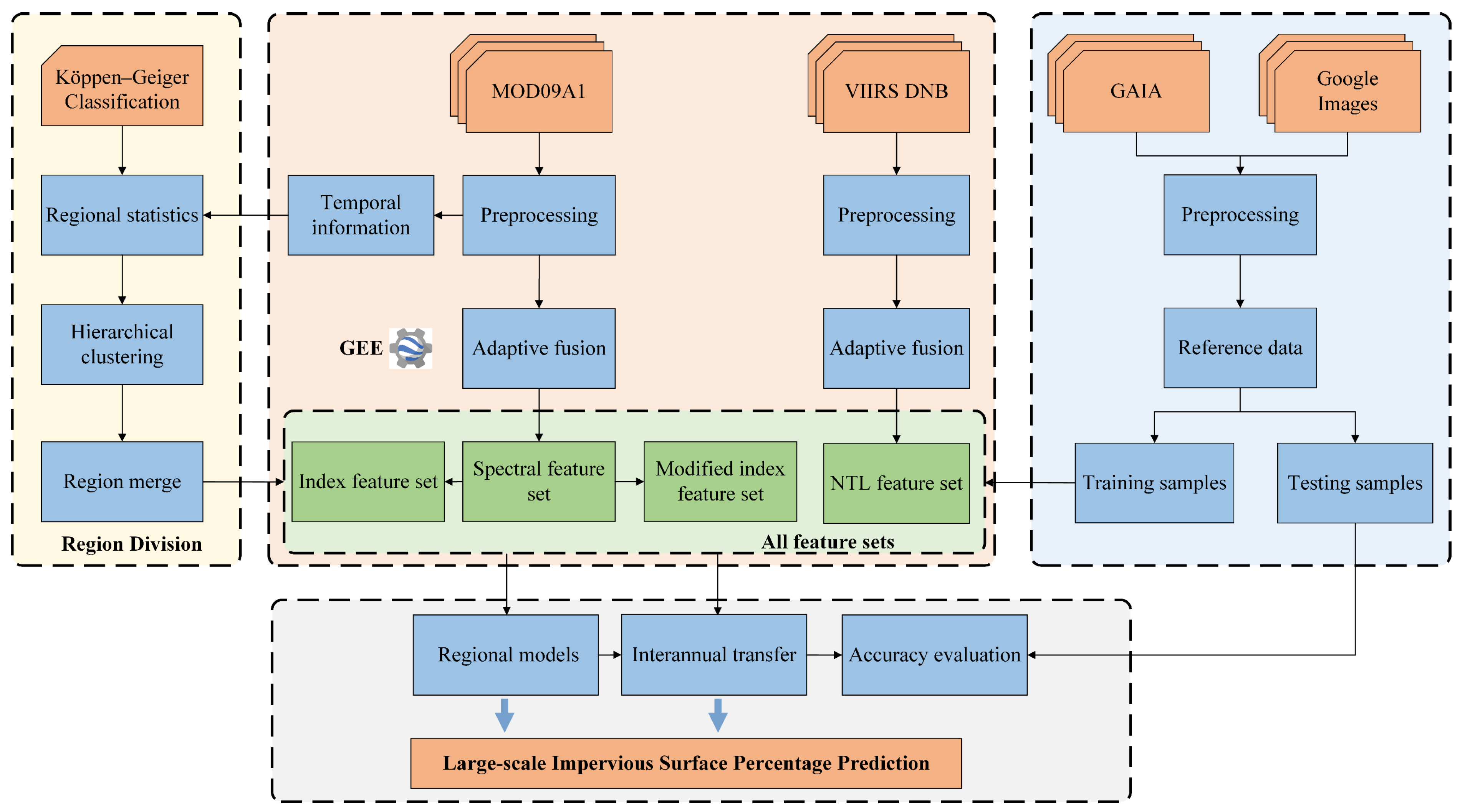
In this study, Asia is used as the study area, as shown in Figure 1. Asia is the largest among the seven continents, with a total area of 4457 × 10⁴ km², and is located 10°S to 80°N latitude and 170°W to 25°E longitude. There are diverse types of ecology and climate including desert climate with sparse vegetation, rainforest climate with continuous high temperature and rainfall, and monsoon climate with alternating rainy and dry seasons. In addition, the landscape is distinctly different in this region and the arid and non-arid characteristics are significant. In addition, the landscape is distinctly different and the arid and non-arid characteristics are significant. Asia covers 48 countries including 5 East Asian countries, 7 South Asian countries, 11 Southeast Asian countries, 5 Central Asian countries, and 20 West Asian countries. In the past few decades, rapid urban population aggregation and urban expansion have occurred in Asia. By 2020, the total population had exceeded 4.5 billion, accounting for 60% of the world’s total population, including an urban population of 2.4 billion accounting for 54% of the world’s urban population. Among them, densely populated areas are mainly distributed in East Asia, Southeast Asia, and South Asia. Large cities and urban agglomerations have been formed with populations of ten million such as Tokyo, Beijing, Shanghai, and Guangzhou. In addition, Asia is one of the regions with the most active economies. Rapid economic development and population growth have accelerated the urbanization of this region, resulting in a dramatic expansion of impervious surfaces.

This study mainly used five types of data including multi-temporal MODIS surface reflectance product (MOD09A1), nighttime lighting product (VIIRS DNB), high-resolution images provided by Google Earth, Köppen–Geiger climate classification data, and global artificial impervious area annual data (GAIA). The details are shown in

Table 1. The details of data used in this study.

Type	Name	Description	Source
Remote Sensing Data	MOD09A1	MODIS Terra/Aqua Surface Reflectance 8-Day Product, 46 periods in a year, spatial resolution 500 m.	https://lpdaac.usgs.gov/ (accessed on 10 February 2022)
	VIIRS DNB	VIIRS DNB Cloud-Free Composites Monthly Product, 12 periods in a year, spatial resolution 500 m.	https://eogdata.mines.edu/products/vnl/ (accessed on 10 February 2022)
Auxiliary Data	Köppen–Geiger climate classification	Köppen–Geiger climate classification global raster data, spatial resolution 1000 m.	http://www.gloh2o.org/koppen/ (accessed on 12 March 2022).
Sample Data	GAIA	Global artificial impervious area products from 1985 to 2018, spatial resolution 30 m.	http://data.ess.tsinghua.edu.cn/ (accessed on 5 January 2022)
	Google Earth historical images	High-resolution historical images. A container collects multi-source data (SPOT5, IKONOS, etc.)	https://earth.google.com/ (accessed on 5 January 2022)

. The data preprocessing mainly included (1) unifying the geographic coordinate system of MOD09A1, VIIRS DNB, and Köppen–Geiger climate classification data; (2) removing noise data from MOD09A1 images [46]; (3) VIIRS DNB data radiometric correction. All data preprocessing was carried out on the Google Earth Engine (GEE) platform. For model training and evaluation, 40,620 samples were manually annotated based on GAIA and high-resolution images from Google Earth.

2.2. Methods

As displayed in Figure 2, the large-scale impervious surface percentage estimation method included three parts: (1) Divide study area based on climate classification data and MODIS time-series data; (2) Adaptively select and fuse time-series images of different regions, then build a feature set based on the fused data for the impervious surface percentage estimation; and (3) Train the estimated models and verify accuracy.

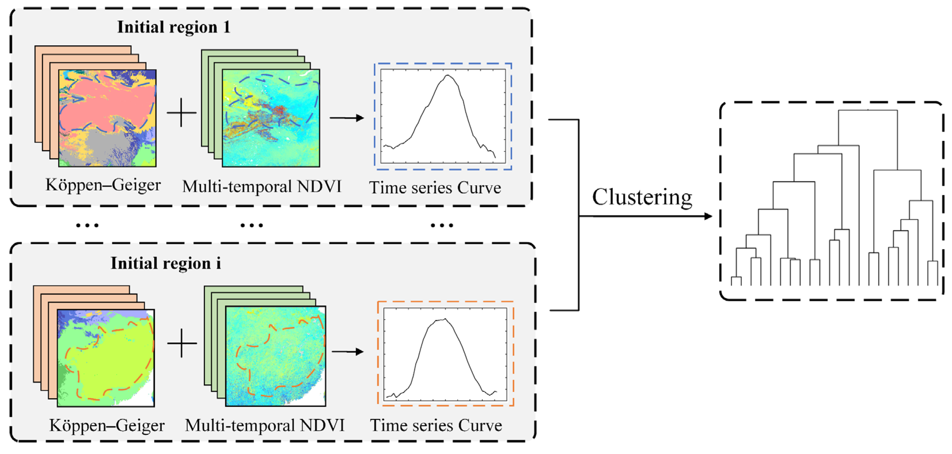
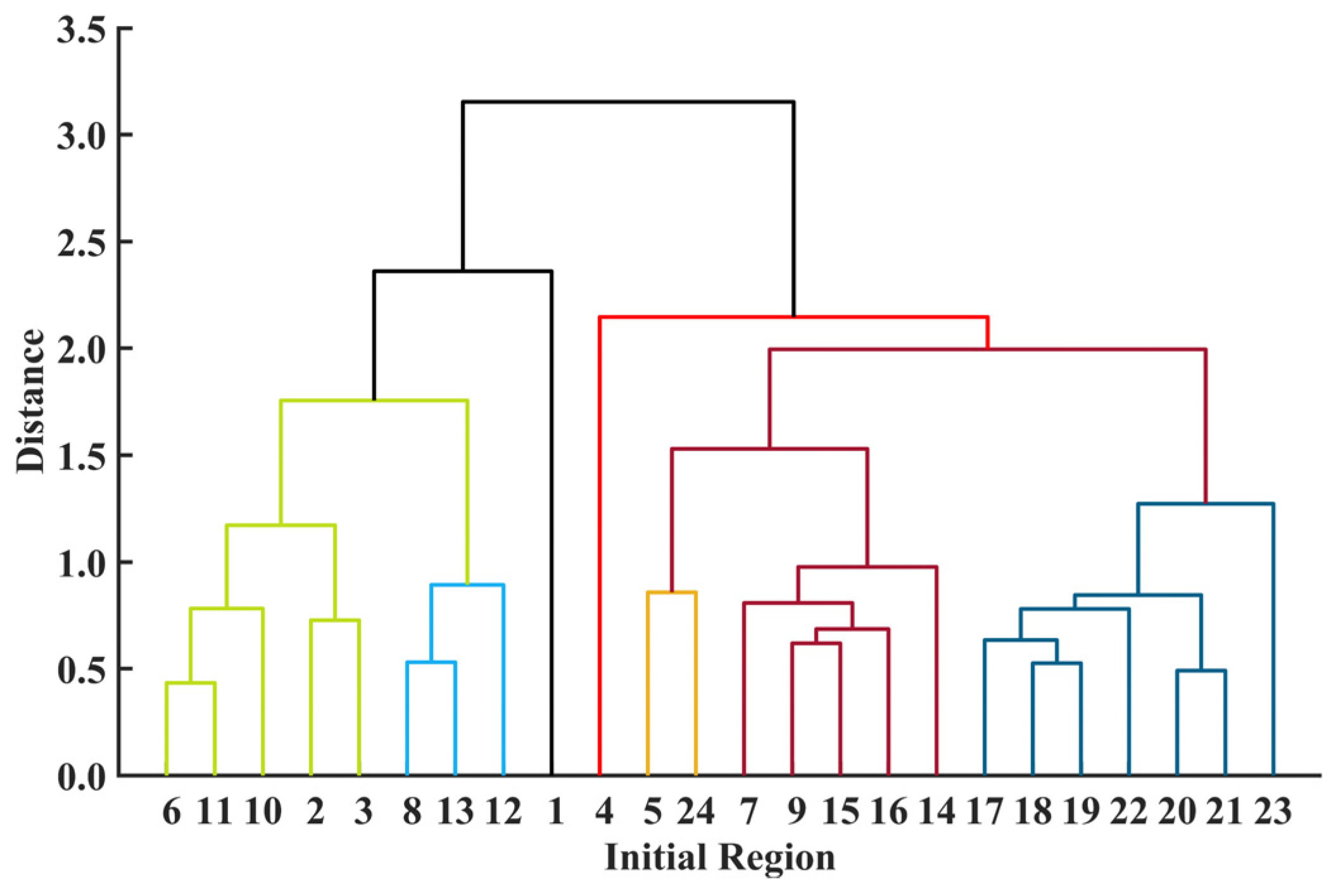
2.2.1. Regional Divisions

In order to overcome the regional climatic and ecological heterogeneity, a regional division method based on the characteristics of regional climate and NDVI time-series data was proposed. Specifically, the Köppen–Geiger climate classification data were used as the climate regional reference [47,48]. This data combine climatic air temperature and precipitation data from multiple independent sources, such as WorldClim, CHELSA, and CHPclim, to map global climate classifications, which can effectively reflect large-scale differences in biome and landscape distribution [49]. Climate factors indirectly affect large-scale regional land cover types and changes, among which vegetation types and differences are the most significant, but cannot specifically reflect the surface information. Therefore, these data are mainly based on traditional natural elements and cannot directly reflect the regional heterogeneities in remote sensing [50]. However, remote sensing images directly express land cover information such as surface spectral reflectance. In addition, NDVI time-series data are often used as a reference for time-series data matching and multi-source data fusion. They are also important indicators for the reflection of the time-series characteristics of surface landscapes and are often used to represent the changes in vegetation phenology [51,52,53,54]. Therefore, based on Köppen–Geiger climate classification data, we conducted regional temporal feature consistency analysis of the time-series NDVI data of different climate types and clustered the climate classification data based on the similarity clustering method to generate the final partition results.

First, to fully reflect the time-series characteristics, based on the annual maximum NDVI composite image from multi-temporal NDVI images, the threshold method was used to select the vegetation cover pixels as the representative pixels. Then, as illustrated in Figure 3, Köppen–Geiger climate classification data were used as the initial regions and the 46-period average NDVI time series for the selected pixels was calculated for each region. In addition, considering the interannual differences, the statistics used multi-year data (2015–2020), and the NDVI for each period was taken from the average of the NDVI in the same period of many years. Finally, the 46-period NDVI time-series curve for each initial region was obtained, and the time series curve for initial region i was calculated:

$${\mathrm{NDVI}}_{\left(i,t\right)}=\mathrm{Mean} \left[ {\mathrm{NDVI}}_{\left(i,t\right)}^{2015},\dots ,{\mathrm{NDVI}}_{\left(i,t\right)}^{2017},\dots ,{\mathrm{NDVI}}_{\left(i,t\right)}^{2020}\right]$$

(1)

$${\mathrm{NDVIs}}_i=\left\{ {\mathrm{NDVI}}_{\left(i,1\right)},\dots ,{\mathrm{NDVI}}_{\left(i,t\right)},\dots ,{\mathrm{NDVI}}_{\left(i,46\right)}\right\}$$

(2)

where ${\mathrm{NDVI}}_{\left(i,t\right)}$ is the NDVI of the initial region i at period t and ${\mathrm{NDVIs}}_i$ is the 46-period NDVI set of the initial region i. Since there are many types of initial regions, the complexity of data processing is increased, which is not conducive to the extraction of large-scale impervious surface information. In addition, there are similar temporal characteristics between regions. Therefore, based on the time series curve of each region, similar regions were merged by hierarchical clustering methods to reduce regional redundancies. The initial regions were adaptively grouped to form new regions:

$$\mathrm{R}=\mathrm{HC}\left({\mathrm{NDVIs}}_1,\dots ,{\mathrm{NDVIs}}_i,\dots ,{\mathrm{NDVIs}}_n\right)$$

(3)

where R is the result of hierarchical clustering.

2.2.2. Time-Series Data Fusion and Feature Construction

In order to construct robust remote sensing features for LISP estimation, multi-temporal remote sensing images were fused. Remote sensing images with vegetation cover seasons are usually used because images from this period can maximize the spectral separability of impervious surfaces from other land cover types [45]. Therefore, to obtain the time window of each new region, a time with high vegetation coverage was selected from the time series curve by the adaptive threshold and the time window was formed:

$${\mathrm{T}}_{\left(i,t\right)}: {\mathrm{NDVI}}_{\left(i,t\right)}\ge {\mathrm{th}}_i$$

(4)

$${\mathrm{th}}_i=\mathrm{Mean}\left({\mathrm{NDVIs}}_i\right)$$

(5)

where ${\mathrm{th}}_i$ is the threshold for region i. When the NDVI of the t-th period is greater than the threshold, the t-th period is selected. Finally, the time window of region i is ${\mathrm{TW}}_i=\left\{{\mathrm{T}}_{\left(i,t\_\mathit{start}\right)},\dots ,{\mathrm{T}}_{\left(i,t\right)},\dots ,{\mathrm{T}}_{\left(i,t\_\mathit{end}\right)}\right\}$. Therefore, multi-temporal images were adaptively selected based on the time window in each region. Then, the selected multi-temporal remote sensing images were composited using the average synthesis algorithm:

$${\mathrm{B}}_m=\mathrm{Mean} \left[ {\mathrm{B}}_m^{t\_\mathit{start}},\dots ,{\mathrm{B}}_m^t,\dots ,{\mathrm{B}}_m^{t\_\mathit{end}}\right]$$

(6)

where m is the number of bands and t is the acquisition period of multi-temporal images, and $t\_\mathit{start}$ and $t\_\mathit{end}$ are the start and end times of the time window of each region. Finally, the spectral feature set was $\mathrm{Ss}=\left\{{\mathrm{B}}_1,{\mathrm{B}}_2,\dots ,{\mathrm{B}}_7\right\}$. The spectral features obtained by average synthesis can smooth the outliers in the single-period image and integrate multiple temporal features to make it more stable in spatiotemporal scales. In addition, to make full use of the spectral information and the difference information between different spectral features, the normalized difference spectral index set (NDSIs) was constructed as the extended feature set:

$$\mathrm{NDSIs}=\left\{\frac{{\mathrm{B}}_m-{\mathrm{B}}_n}{{\mathrm{B}}_m+{\mathrm{B}}_n}|m,n=1,\cdots 7,m\ne n\right\}$$

(7)

where ${\mathrm{B}}_m$ and ${\mathrm{B}}_n$ are the m-th and n-th features in the synthetic spectral data, respectively. The NDSIs refer to the NDVI construction method and incorporate more spectral difference information. Moreover, by modifying the parameters, the soil-adjusted vegetation index (SAVI) highlights the difference between the major information and the background. Furthermore, to maximize the distinction between different land covers, this paper proposed the modified normalized index feature set (MNDSIs) construction method based on SAVI:

$$\mathrm{MNDSIs}=\left\{\frac{{\mathrm{B}}_m-{\mathrm{B}}_n}{{\mathrm{B}}_m+{\mathrm{B}}_n+\mathrm{L}}\left(1+\mathrm{L}\right)|m,n=1,\cdots 7,m\ne n\right\}$$

(8)

where ${\mathrm{B}}_m$ and ${\mathrm{B}}_n$ are the m-th and n-th features in the synthetic spectral data, respectively, and the modified parameter is L = 0.5. NTL data are closely related to human production activities and show potential in large-scale impervious surface applications and the NTL features were added [31,55]. In addition, to ensure the consistency of the observation time, the multi-temporal NTL data were also applied to the same period of the MODIS data. Then, the NTL features were obtained by average synthesis.

Effective features are the key to extracting impervious surfaces accurately. Different features and feature combinations have different effects on other regions. To compare the above feature set and combined feature sets in the impervious surface percentage estimation, five schemes were designed in this paper, as shown in

Table 2. Feature set combination scheme.

Scheme	Feature Set Combination
1	Ss
2	Ss + NDSIs
3	Ss + MNDSIs
4	Ss + NDSIs + NTL
5	Ss + MNDSIs + NTL

.

2.2.3. Development of Prediction Models

In the estimation model building stage, five regression models were employed including multiple linear regression (MLR), random forest regression (RFR), support vector machine regression (SVR), regression neural network (RNN), and Gaussian process regression (GPR). For the RFR model, the number of decision trees is set to 100. The Gaussian kernel is used in the SVR model. A narrow neural network regression model is constructed. The regression kernel function is an exponential kernel in the GPR model. During the experiment, global and regional models were constructed separately to evaluate the impact of regional divisions on the large-scale impervious surface percentage prediction [18]. The global model was trained using all training samples in the entire study area. In contrast, regional models only used the training data within each region to train the model. We manually annotated 4000 to 7000 samples within each region. When training the global model, 80% of the samples in all regions were used as training samples and the remaining 20% were used for testing. The same training setup was used to train the regional model, selecting 80% of the samples in each region for training and the remaining samples for testing.

2.2.4. Accuracy Evaluation

The results are evaluated using two accuracy metrics including coefficient of determination (R²) and root mean squared error (RMSE), which are defined as

$${\mathrm{R}}^2=1-\frac{{\sum }_{i=1}^n{({\hat{y}}_i-y_i)}^2}{{\sum }_{i=1}^n{({\overline{y}}_i-y_i)}^2}$$

(9)

$$\mathrm{RMSE}=\sqrt{\frac{1}{n}{\sum }_{i=1}^n{(y_i-{\hat{y}}_i)}^2}$$

(10)

where $y_i$ is the real value, ${\overline{y}}_i$ is the mean of the data set, and ${\hat{y}}_i$ is the predicted value. In the evaluation of model transfer performance, the model prediction results are evaluated using the labeled samples of the target domain, and the above two evaluation metrics are also used.

3. Results

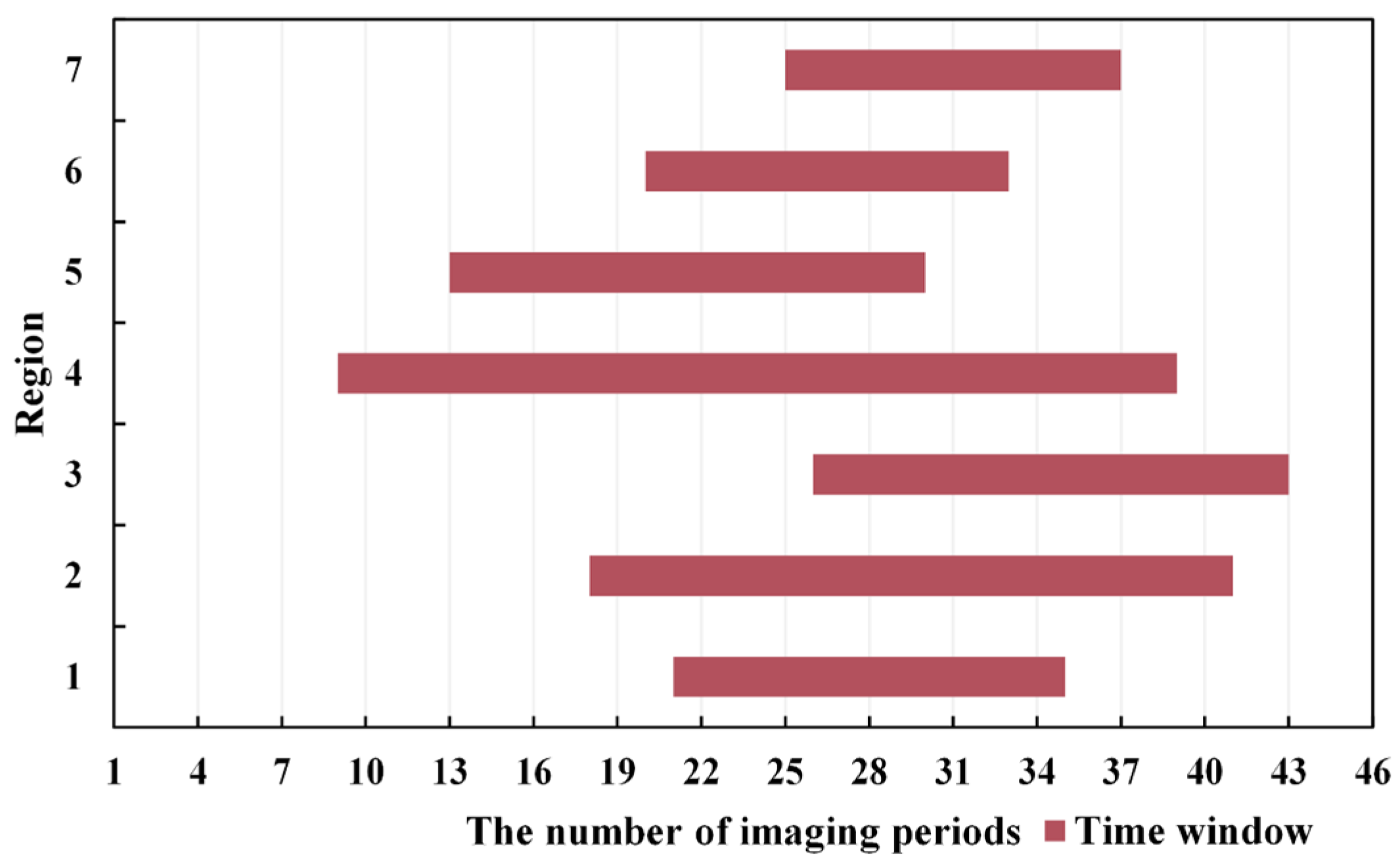
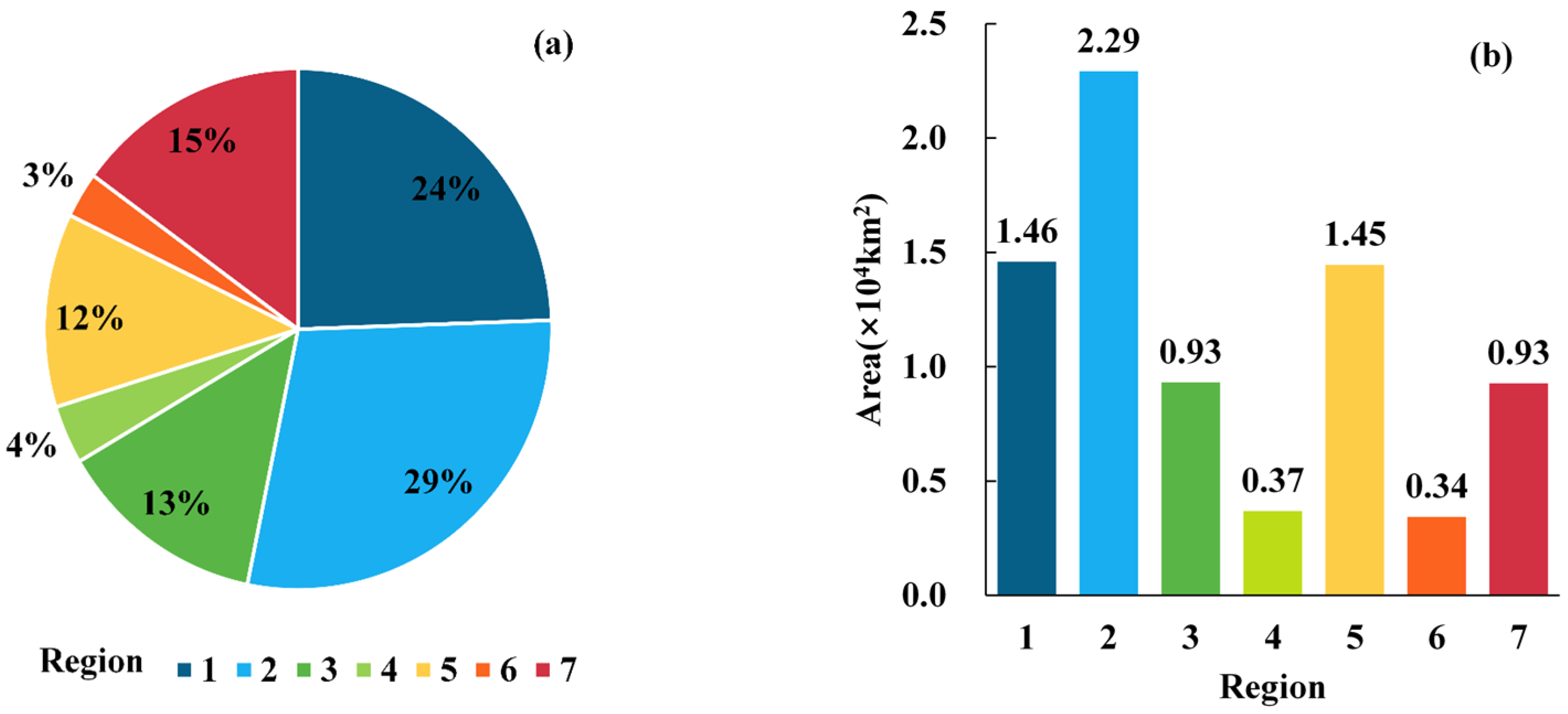
3.1. Region Division Results

The study area was spatially divided according to the constructed regional division method. There were a total of 21 climate types in Asia, which are defined as the initial regions. Figure 4 shows the hierarchical clustering results; the clustering threshold was set to 1.5 and Asia was divided into seven regions. These regions and time windows for each region are shown in Figure 5 and Figure 6. It can be seen in Figure 5 that regions 1 and 2 are mainly located in East Asia (excluding Northwest China), dominated by monsoon climates with significant seasonal characteristics. Among them, region 2 has a high air temperature and precipitation in summer and the vegetation growth period is long, resulting in a significantly longer time window than region 1. With decreasing latitude, the air temperature is no longer the main factor affecting vegetation growth. Therefore, region 3 is mainly distributed in South Asia and the Indochina Peninsula. The time window is the period between the end of the rainy season and the beginning of the dry season. During this period, the vegetation is still growing and the cloud cover is decreasing, which is the best period to obtain remote sensing images. Region 4 is located in the Malay Archipelago. Due to the high air temperature and precipitation throughout the year, a shorter observation period cannot be selected. Therefore, the time window is the longest of all regions. Regions 5 and 6 include arid or semi-arid regions in Central Asia, Northwest Asia, and Northwest China, with significant air temperature differences and low precipitation throughout the year. The time windows for regions 5 and 6 occur during periods with high air temperatures and less cloud cover. Region 7 is mainly a desert area in Southwest Asia, and most areas have a high air temperature and no precipitation almost throughout the year. The time window occurs because there is still a small amount of vegetation in the region.

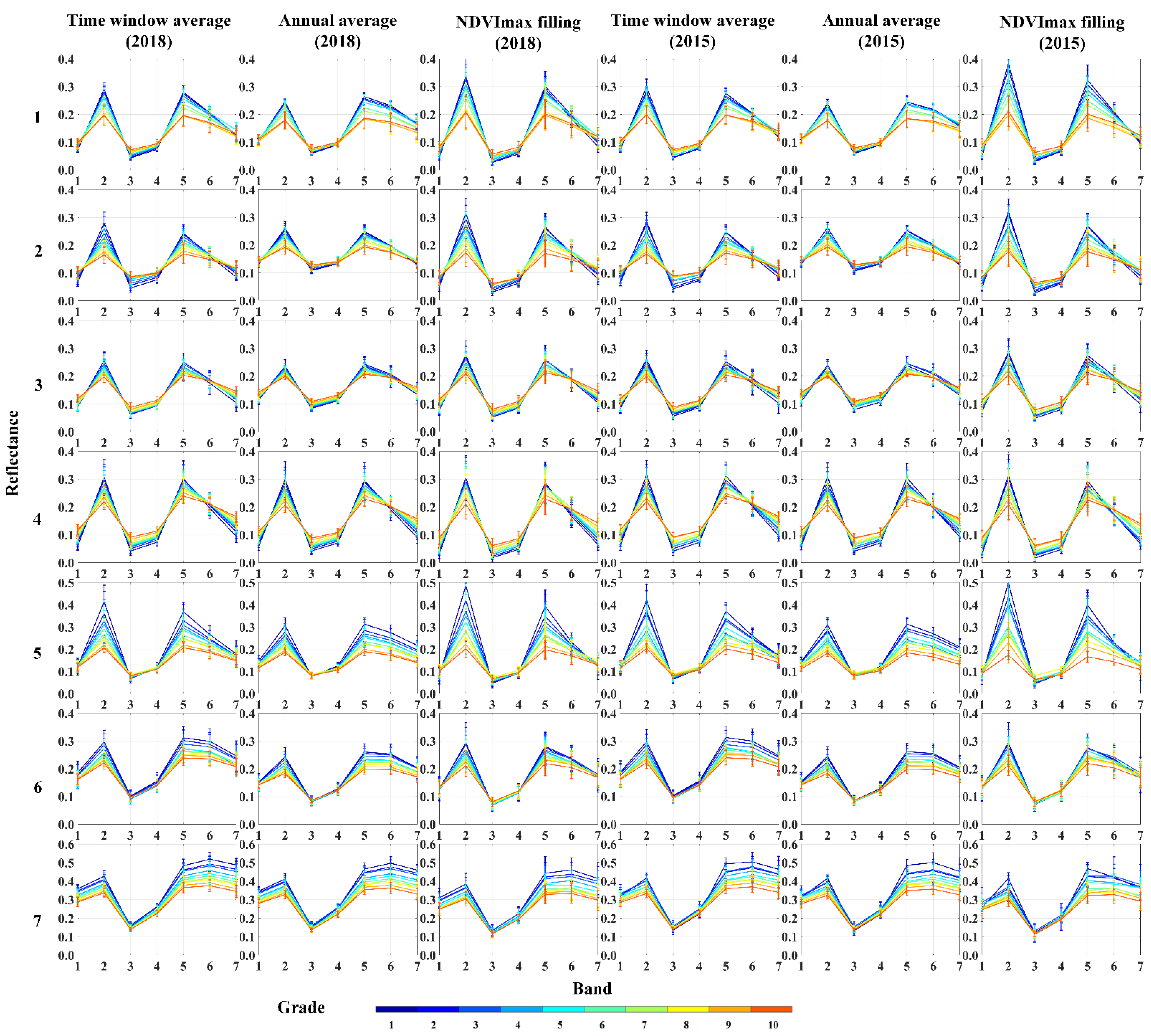
3.2. Comparison of Time-Series Image Synthesis Methods

To verify the advantages of the time-series image synthesis method proposed, this method was compared with the annual average synthesis method and the NDVImax filling synthesis method. Among them, the NDVImax filling image was obtained by filling each pixel with the data that have the highest NDVI in the annual images [56]. The spectral curves of the impervious surface percentage obtained were analyzed using different methods. Firstly, 1000–2000 samples were randomly selected from each of the seven regions. These samples were then divided into ten groups, ranging from 0 to 1, with an interval of 0.1. Finally, we calculated the mean values and standard deviations of the spectral features in each group to form 10 grades.

Figure 7 shows the image synthesis methods in 2015 and 2018. The NDVImax filling synthesis method can enhance the feature expression with more significant visual changes such as in Bands 2 and 5. However, the more significant standard deviations reflect poorer stability of the same grade samples. In addition, the spectral curves synthesized using this method have poor consistency in different years, which was not conducive to the application of interannual transfer. For example, the spectral curves for 2015 and 2018 are less similar in region 5. Although the annual average synthesis method effectively reduces the standard deviation and smooths out abnormal data, the annual average also weakens the unique time-series characteristics. Therefore, in the time window average synthesis method for the same band, reflectance differences between different curves are more evident than in the annual average synthesis method. For example, the range of Band 2 is 0.18–0.29 in region 1 but the annual average synthesis method is 0.16–0.23. In addition, the spectral curve has more apparent differences between different bands, enhancing feature identification and providing conditions for constructing index features. For instance, for region 2, the grade 1 curve has reflectances of 0.27 and 0.11 for bands 2 and 3, respectively, based on the annual average synthesis method. However, using our proposed method, the reflectances are 0.29 and 0.05 and the difference value is 0.24. Therefore, the time window average synthesis method can highlight differences in land cover types and obtain more stable time-series features. Finally, limited by the large-scale landscape differences, spectral curves show different shapes in different regions, which indicates the necessity for regional divisions.

3.3. Estimation Results of Different Feature Set Combinations

The RFR was used as the model to evaluate the results of different feature set combinations for estimating the impervious surface percentage [57]. In this study, the difference information between different spectral features was used. As can be seen in

Table 3. Results of feature set combinations in different regions (R²).

Region	Scheme 1	Scheme 2	Scheme 3	Scheme 4	Scheme 5	LISI
1	0.8386	0.8449	0.8440	0.8517	0.8525	0.7014
2	0.8313	0.8411	0.8405	0.8473	0.8464	0.6548
3	0.8319	0.8495	0.8487	0.8511	0.8502	0.6170
4	0.8106	0.8351	0.8321	0.8475	0.8444	0.5275
5	0.8022	0.8368	0.8404	0.8442	0.8495	0.6146
6	0.7981	0.8342	0.8406	0.8445	0.8510	0.6017
7	0.7632	0.8318	0.8402	0.8446	0.8552	0.6512
ALL	0.7884	0.8218	0.8205	0.8269	0.8286	0.6231

, schemes that fuse the spectral feature set, index feature set, or modified index feature set were more accurate than the spectral feature set. Among them, scheme 3 performed better in arid and semi-arid regions (such as regions 6 and 7). In addition, the NTL had no obvious brightness information in the bare soil areas outside the city, which was in contrast with the highlight phenomenon in the urban area [58,59,60,61]. Therefore, after combining the NTL features, the increment of R² in arid and semi-arid regions (regions 6 and 7) was higher than in regions with vegetation coverage (regions 1, 2, 3, and 4) [30]. Finally, the LISI (large-scale impervious surface index) was involved in the comparison [25]. This indexing feature was established based on NDVI and NTL, and it is often used for large-scale impervious surface extraction. The results generally illustrated that our proposed multi-feature set combination scheme showed better estimation performance overall and had regional advantages.

3.4. Comparison of Impervious Surface Percentage Estimation Models

As shown in

Table 4. Prediction results of different models based on regional divisions.

Region	RFR		SVR		RNN		GPR		MLR
	R2	RMSE	R2	RMSE	R2	RMSE	R2	RMSE	R2	RMSE
1	0.8518	0.1376	0.8516	0.1399	0.8580	0.1393	0.8589	0.1359	0.8046	0.1605
2	0.8481	0.1323	0.8455	0.1341	0.8427	0.1355	0.8549	0.1294	0.7915	0.1549
3	0.8505	0.1187	0.8550	0.1176	0.8551	0.1175	0.8617	0.1144	0.8046	0.1598
4	0.8485	0.1322	0.8440	0.1344	0.8453	0.1337	0.8571	0.1298	0.7916	0.1549
5	0.8494	0.1189	0.8507	0.1174	0.8481	0.1186	0.8587	0.1156	0.7955	0.1585
6	0.8505	0.1295	0.8502	0.1283	0.8492	0.1279	0.8592	0.1205	0.8155	0.1588
7	0.8554	0.1401	0.8555	0.1401	0.8578	0.1399	0.8618	0.1329	0.8015	0.1596
ALL	0.8202	0.1452	0.8190	0.1481	0.8163	0.1498	0.8326	0.1415	0.7212	0.1853

, regional models are better than global models. Global samples are not suitable for global models on large scales due to inevitable landscape differences. However, the regional model more intensively expresses the feature information of similar landscapes, which is more accurate and stable. The R² of the same kind of model was similar in the different regions, which shows that our proposed regional divisions had better rationality. For instance, in the GPR model, the R² was between 0.855 and 0.865 for all regions. Except for MLR, the R² of the other models was above 0.80, indicating the applicability of the combined feature sets to the different models. In general, the prediction results of the GPR were the best, and for each region were better than the other kinds of models; MLR was the worst and the R² was 0.790 at its lowest; RFR, SVR, and RNN were similar and the R² was between 0.840 and 0.860.

The map of impervious surface percentages in Asia based on the GPR model is shown in Figure 8. The impervious surface shows a decreasing trend from east to west in Asia and can be divided into three parts. In East Asia, impervious surfaces are dense and compact, especially in coastal cities, large cities, or urban agglomerations. In addition, due to economic and population constraints, the impervious surfaces are fragmented in countries in Northwest China and Central Asia. Finally, West Asia is limited by the natural environment and ecosystem, and the impervious surface percentage is generally lower than in other regions. On the urban scale, due to differences in natural conditions and economic development, the distribution is diverse in different cities. In economically developed cities, such as Tokyo and Shanghai, the overall distribution is more expansive, and the impervious surface percentage is higher in urban centers. In addition, cities such as New Delhi and Jakarta have large populations and concentrated urban functions and impervious surfaces are also widely concentrated in urban areas. However, small and medium-scale cities with low economic development and low population density, such as Ankara and Ashgabat, have scattered distributions and their overall area is smaller than large cities.

3.5. Evaluation of Interannual Transferability

The model was used as the baseline model in 2018 and was applied to 2015 and 2020 data. Due to sensor aging and the external environment, there were some differences in the interannual remote sensing data. Therefore, the data for other years were corrected by histogram matching based on different regions. Since the results of the GPR in the above models were the best, the model was selected for transfer testing. In

Table 5. Transferability results from uncorrected and corrected.

Region	unCorr (2015)		Corr (2015)		unCorr (2020)		Corr (2020)
	R2	RMSE	R2	RMSE	R2	RMSE	R2	RMSE
1	0.8279	0.1463	0.8398	0.1415	0.8296	0.1479	0.8405	0.1427
2	0.8205	0.1426	0.8332	0.1350	0.8215	0.1450	0.8354	0.1373
3	0.8120	0.1352	0.8275	0.1305	0.8127	0.1342	0.8286	0.1311
4	0.8234	0.1410	0.8354	0.1331	0.8254	0.1395	0.8376	0.1311
5	0.8239	0.1405	0.8327	0.1344	0.8248	0.1409	0.8335	0.1357
6	0.8276	0.1492	0.8321	0.1432	0.8261	0.1487	0.8343	0.1439
7	0.8165	0.1534	0.8247	0.1468	0.8197	0.1528	0.8279	0.1479

, without interannual correction, the R² of all models is between 0.810 and 0.830 in the different regions of the transferred year. After region-based interannual correction, the R² of all models was improved to 0.825–0.845.

Figure 9 and Figure 10 show the impervious surface area in Asia from 2015 to 2020. Among them, the impervious surface area and expansion area of region 2 are the largest. Regions 4 and 6 have the smallest impervious surface and extension areas. Furthermore, our results were compared with other products to verify the prediction effect. Existing impervious surface products include GAIA, NUACI, and GHSL [39]. NUACI is a global multi-temporal impervious surface 30 m product [45]. GHSL is a multi-resolution product that has been used to describe manmade built-up areas in the past 40 years [62,63]. Figure 10 shows our method, GAIA, NUACI, and GHSL for impervious surface areas in Asia. Among them, the results of this paper are lower than GAIA and slightly higher than GHSL and NUACI, and the overall change trend is the same as in GAIA from 2015 to 2018.

4. Discussion

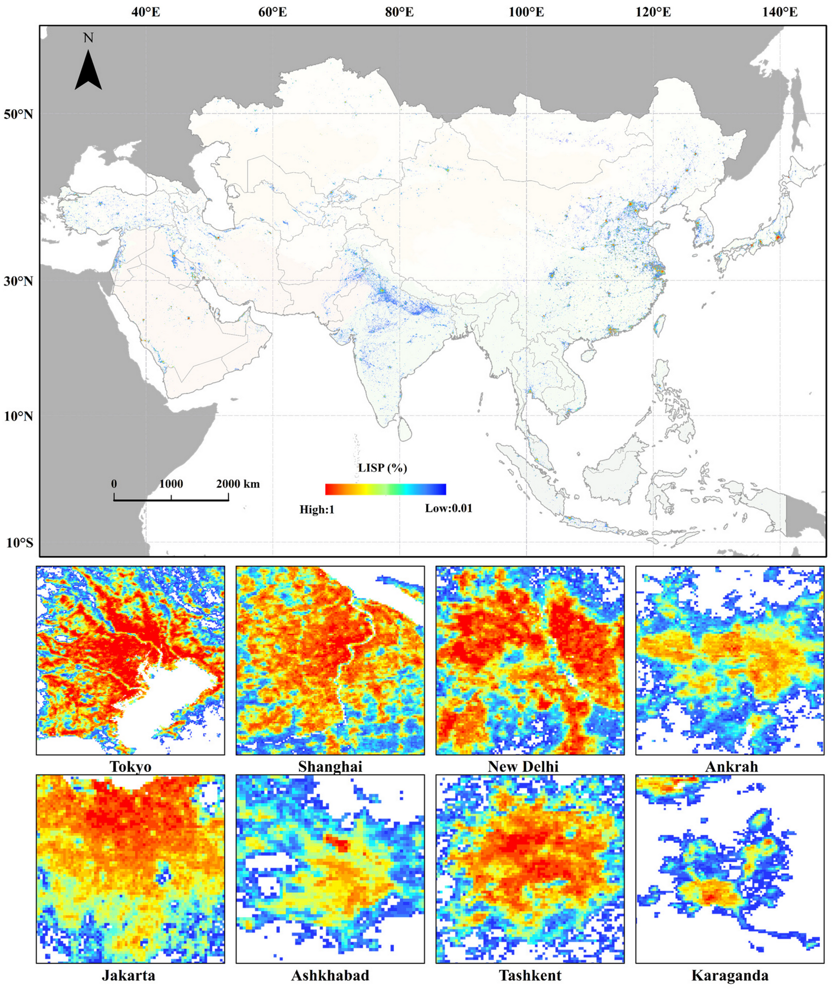
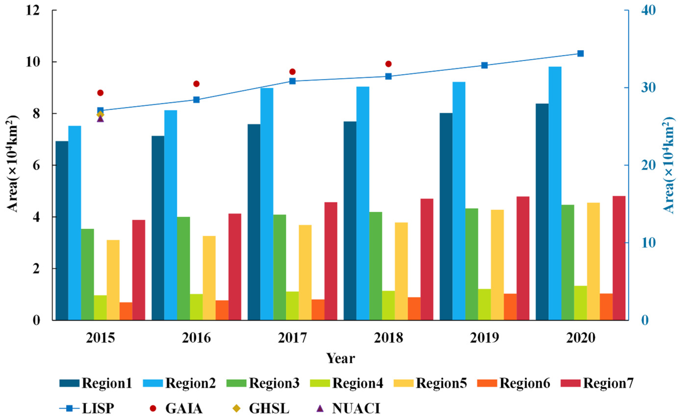
4.1. Comparison with Other Impervious Surface Products

To further validate our method quantitatively, the prediction results were compared with existing impervious surface products. This study selected GAIA data in 2015 (GAIA-2015), GHSL data in 2015 (GHSL-2015), and NUACI data in 2015 (NUACI-2015). In addition, GLC_FCS30 is a global 30m fine classification system land cover product, and impervious surface data were selected from 2020 (GLC-2020) [18]. Other datasets were converted to impervious surface percentage data with the same spatial resolution. Subsequently, 1000–2000 samples were randomly selected in 2015 or 2020 to evaluate each region, and R² and RMSE were used as the evaluation metrics. The results are shown in

Table 6. Accuracy of the five impervious surface products.

Region	LISP-2015		GAIA-2015		GHSL-2015		NUACI-2015		LISP-2020		GLC-2020
	R2	RMSE	R2	RMSE	R2	RMSE	R2	RMSE	R2	RMSE	R2	RMSE
1	0.8402	0.1406	0.7498	0.2009	0.8111	0.1473	0.5845	0.2495	0.8380	0.1413	0.8329	0.1382
2	0.8336	0.1323	0.7684	0.1992	0.8272	0.1350	0.7433	0.1860	0.8348	0.1355	0.8349	0.1388
3	0.8249	0.1329	0.8095	0.1413	0.7912	0.1518	0.6367	0.1920	0.8216	0.1315	0.7681	0.1681
4	0.8314	0.1372	0.8282	0.1422	0.8071	0.1455	0.5784	0.2292	0.8336	0.1397	0.7846	0.1436
5	0.8326	0.1389	0.7889	0.1488	0.7867	0.1695	0.4835	0.2164	0.8343	0.1386	0.8081	0.1474
6	0.8335	0.1415	0.8016	0.1486	0.7925	0.1625	0.5047	0.2059	0.8352	0.1394	0.8023	0.1518
7	0.8269	0.1431	0.8185	0.1457	0.7842	0.1552	0.3134	0.4449	0.8293	0.1459	0.7784	0.1543

and the standard year model was applied to 2015 and 2020, with R² ranging from 0.820 to 0.840. The accuracy of each region was similar, and the overall results were higher than other products. The NUACI-2015 had the lowest accuracy for all regions. In addition, the NUACI data cannot effectively distinguish between impervious surfaces and bare soil in regions with low vegetation coverage (regions 5, 6, 7) [45]. With another product, the R² of GAIA-2015 was 0.750 and 0.768 in regions 1 and 2, respectively, which was lower than the other regions in GAIA [39]. Due to rapid developments in the past decade, impervious and pervious surfaces frequently change within a short period, resulting in low accuracy. Compared with other products, the GHSL-2015 had no significant difference in the R² of the seven regions (0.780–0.830) but overall accuracy is lower than LISP. The R² was above 0.830 for regions 1 and 2 for the GLC-2020, which was close to LISP, but the R² in other regions was lower than 0.810. Generally speaking, compared with high-resolution impervious surface products, the spatial resolution of the impervious surface percentage data was not high in this study. However, the data showed better stability in different regions and the model can be transferred between different years. The experimental results also showed that due to the multi-source data used by high-resolution products, there are some problems such as time-series inconsistencies and obvious temporal and spatial differences in the data, which led to large spatial differences in product accuracy.

To show the differences between the impervious surface products, we visually compared our predictions with other products. Among them, seven typical cities were selected, including large cities and small-scale cities. In Figure 11, it can be seen that NUACI-2015 ignored rural information (Beijing), did not extract complete impervious surface information (Tehran), and overestimated urban areas (Singapore). The possible reason is that based on a threshold method, NUACI limited the distinction between impervious and pervious surfaces. In addition, the overall impervious surface percentage of GHSL-2015 was lower than in the other products, especially in the cloudy and rainy regions with high vegetation coverage (Singapore). In addition, GAIA performed poorly in sparsely vegetated areas and was easily confused with bare land (Urumqi and Tehran). Moreover, some details were lost in cloudy and rainy areas (Haiphong). Finally, because GLC-2020 did not adequately distinguish impervious surfaces from bare soil, impervious surfaces were significantly overestimated in sparsely vegetated cities (Tehran and Riyadh).

In Figure 11, it can be seen that LISP-2015 and LISP-2020 reflected the impervious surface percentage change process from 2015 to 2020. Generally, the impervious surface of the city center does not change much. For economically developed cities, the growth area of impervious surfaces was mainly the non-central area of the city (Beijing and Guangzhou). In addition, the natural environment is also an essential factor affecting the urbanization process. Singapore is a developed country city and Riyadh is a developing country city but both are limited by terrain and resources. The distribution of impervious surfaces is stable and the expansion is insignificant.

4.2. Advantages and Limitations

In the extraction of large-scale impervious surfaces, the heterogeneity of the landscape leads to different challenges in different regions. For example, impervious surfaces are difficult to distinguish from bare land in arid and semi-arid climates. Furthermore, there are different extraction results because of seasonal land cover changes in monsoon regions. To this end, we combined the spatial differences in the landscapes represented by the Köppen–Geiger climate classification with the time-series characteristics reflected by the NDVI multitemporal data. The large-scale regional division method was explored based on data fusion and consistency analysis to solve the above problems. Furthermore, the proposed method generated continuous regions and reduced regional redundancies, which was the premise of building regional stability models. The regional division results were influenced by the Köppen–Geiger climate regions and vegetation growth characteristics. Secondly, this study constructed robust feature sets and suitable feature set combinations for different regions and optimizing feature set combinations improved the prediction in sparsely vegetated regions. Since the estimation model was constructed based on consistent regional and stable features, the model can be transferred between different years and obtain better estimation results. This study used MODIS images to estimate the impervious surface percentages, which have a coarser spatial resolution. The underestimation of impervious surface percentages occurs in areas with scattered impervious surfaces, such as sparsely distributed buildings and roads between mountains. In addition, the VIIRS DNB data are nighttime light data recorded in the past ten years. Other data still need to be used as references for the dynamic monitoring of large-scale impervious surface percentages for up to 20 years.

5. Conclusions

This study aims to solve the problem of regional differences in the extraction of large-scale impervious surface information and build more accurate large-scale impervious surface percentage estimation models. For this purpose, by fully considering the consistency of climate types and time-series NDVI features, a regional division method is proposed to divide the whole of Asia into several regions. Then, based on the adaptive selection and fusion of regional time-series images, a feature set for impervious surface percentage estimation is constructed. The experimental results indicate that the proposed regional division method and feature construction method can effectively overcome the negative influences of spatiotemporal heterogeneity on the estimation results and significantly improve the estimation accuracy of impervious surface percentages. Moreover, compared with other products, our proposed method exhibits better regional accuracy and global equalization.

References

1. Arnold, C.L., Jr.; Gibbons, C.J. Impervious surface coverage: The emergence of a key environmental indicator. J. Am. Plan. Assoc. 1996, 62, 243–258. [Google Scholar] [CrossRef]
2. Chithra, S.; Nair, M.H.; Amarnath, A.; Anjana, N. Impacts of impervious surfaces on the environment. Int. J. Eng. Sci. Invent. 2015, 4, 27–31. [Google Scholar]
3. Li, X.; Zhou, Y.; Eom, J.; Yu, S.; Asrar, G.R. Projecting global urban area growth through 2100 based on historical time series data and future Shared Socioeconomic Pathways. Earth’s Future 2019, 7, 351–362. [Google Scholar] [CrossRef] [Green Version]
4. Schneider, A.; Chang, C.; Paulsen, K. The changing spatial form of cities in Western China. Landsc. Urban Plan. 2015, 135, 40–61. [Google Scholar] [CrossRef]
5. Shao, Z.; Fu, H.; Li, D.; Altan, O.; Cheng, T. Remote sensing monitoring of multi-scale watersheds impermeability for urban hydrological evaluation. Remote Sens. Environ. 2019, 232, 111338. [Google Scholar] [CrossRef]
6. Yang, J.; Siri, J.G.; Remais, J.V.; Cheng, Q.; Zhang, H.; Chan, K.K.; Sun, Z.; Zhao, Y.; Cong, N.; Li, X.; et al. The Tsinghua–Lancet Commission on Healthy Cities in China: Unlocking the power of cities for a healthy China. Lancet 2018, 391, 2140–2184. [Google Scholar] [CrossRef] [Green Version]
7. Feng, S.; Fan, F. Impervious surface extraction based on different methods from multiple spatial resolution images: A comprehensive comparison. Int. J. Digit. Earth 2021, 14, 1148–1174. [Google Scholar] [CrossRef]
8. Sugg, Z.P.; Finke, T.; Goodrich, D.C.; Moran, M.S.; Yool, S.R. Mapping impervious surfaces using object-oriented classification in a semiarid urban region. Photogramm. Eng. Remote Sens. 2014, 80, 343–352. [Google Scholar] [CrossRef] [Green Version]
9. Sebari, I.; He, D.-C. Automatic fuzzy object-based analysis of VHSR images for urban objects extraction. ISPRS J. Photogramm. Remote Sens. 2013, 79, 171–184. [Google Scholar] [CrossRef]
10. Fu, Y.; Liu, K.; Shen, Z.; Deng, J.; Gan, M.; Liu, X.; Lu, D.; Wang, K. Mapping impervious surfaces in town–rural transition belts using China’s GF-2 imagery and object-based deep CNNs. Remote Sens. 2019, 11, 280. [Google Scholar] [CrossRef] [Green Version]
11. Xu, J.; Zhao, Y.; Zhong, K.; Zhang, F.; Liu, X.; Sun, C. Measuring spatio-temporal dynamics of impervious surface in Guangzhou, China, from 1988 to 2015, using time-series Landsat imagery. Sci. Total Environ. 2018, 627, 264–281. [Google Scholar] [CrossRef] [PubMed]
12. Deng, C.; Wu, C. A spatially adaptive spectral mixture analysis for mapping subpixel urban impervious surface distribution. Remote Sens. Environ. 2013, 133, 62–70. [Google Scholar] [CrossRef]
13. Sun, G.; Chen, X.; Ren, J.; Zhang, A.; Jia, X. Stratified spectral mixture analysis of medium resolution imagery for impervious surface mapping. Int. J. Appl. Earth Obs. Geoinf. 2017, 60, 38–48. [Google Scholar] [CrossRef] [Green Version]
14. Zhang, H.; Lin, H.; Wang, Y. A new scheme for urban impervious surface classification from SAR images. ISPRS J. Photogramm. Remote Sens. 2018, 139, 103–118. [Google Scholar] [CrossRef]
15. Huang, X.; Song, Y.; Yang, J.; Wang, W.; Ren, H.; Dong, M.; Feng, Y.; Yin, H.; Li, J. Toward accurate mapping of 30-m time-series global impervious surface area (GISA). Int. J. Appl. Earth Obs. Geoinf. 2022, 109, 102787. [Google Scholar] [CrossRef]
16. Zhang, X.; Liu, L.; Zhao, T.; Gao, Y.; Chen, X.; Mi, J. GISD30: Global 30 m impervious-surface dynamic dataset from 1985 to 2020 using time-series Landsat imagery on the Google Earth Engine platform. Earth Syst. Sci. Data 2022, 14, 1831–1856. [Google Scholar] [CrossRef]
17. Gong, P.; Wang, J.; Yu, L.; Zhao, Y.; Zhao, Y.; Liang, L.; Niu, Z.; Huang, X.; Fu, H.; Liu, S.; et al. Finer resolution observation and monitoring of global land cover: First mapping results with Landsat TM and ETM+ data. Int. J. Remote Sens. 2013, 34, 2607–2654. [Google Scholar] [CrossRef] [Green Version]
18. Zhang, X.; Liu, L.; Wu, C.; Chen, X.; Gao, Y.; Xie, S.; Zhang, B. Development of a global 30 m impervious surface map using multisource and multitemporal remote sensing datasets with the Google Earth Engine platform. Earth Syst. Sci. Data 2020, 12, 1625–1648. [Google Scholar] [CrossRef]
19. Chen, J.; Chen, J.; Liao, A.; Cao, X.; Chen, L.; Chen, X.; He, C.; Han, G.; Peng, S.; Lu, M.; et al. Global land cover mapping at 30 m resolution: A POK-based operational approach. ISPRS J. Photogramm. Remote Sens. 2015, 103, 7–27. [Google Scholar] [CrossRef] [Green Version]
20. Roy, D.P.; Ju, J.; Kline, K.; Scaramuzza, P.L.; Kovalskyy, V.; Hansen, M.; Loveland, T.R.; Vermote, E.; Zhang, C. Web-enabled Landsat Data (WELD): Landsat ETM+ composited mosaics of the conterminous United States. Remote Sens. Environ. 2010, 114, 35–49. [Google Scholar] [CrossRef]
21. Ju, J.; Roy, D.P. The availability of cloud-free Landsat ETM+ data over the conterminous United States and globally. Remote Sens. Environ. 2008, 112, 1196–1211. [Google Scholar] [CrossRef]
22. Zhang, C.; Li, W.; Travis, D. Gaps-fill of SLC-off Landsat ETM+ satellite image using a geostatistical approach. Int. J. Remote Sens. 2007, 28, 5103–5122. [Google Scholar] [CrossRef]
23. Tian, Y.; Chen, H.; Song, Q.; Zheng, K. A novel index for impervious surface area mapping: Development and validation. Remote Sens. 2018, 10, 1521. [Google Scholar] [CrossRef] [Green Version]
24. Tang, Y.; Shao, Z.; Huang, X.; Cai, B. Mapping Impervious Surface Areas Using Time-Series Nighttime Light and MODIS Imagery. Remote Sens. 2021, 13, 1900. [Google Scholar] [CrossRef]
25. Guo, W.; Lu, D.; Wu, Y.; Zhang, J. Mapping impervious surface distribution with integration of SNNP VIIRS-DNB and MODIS NDVI data. Remote Sens. 2015, 7, 12459–12477. [Google Scholar] [CrossRef] [Green Version]
26. Lu, D.; Tian, H.; Zhou, G.; Ge, H. Regional mapping of human settlements in southeastern China with multisensor remotely sensed data. Remote Sens. Environ. 2008, 112, 3668–3679. [Google Scholar] [CrossRef]
27. Guo, W.; Li, G.; Ni, W.; Zhang, Y.; Lu, D. Exploring improvement of impervious surface estimation at national scale through integration of nighttime light and proba-v data. GIScience Remote Sens. 2018, 55, 699–717. [Google Scholar] [CrossRef]
28. Ma, Q.; He, C.; Wu, J.; Liu, Z.; Zhang, Q.; Sun, Z. Quantifying spatiotemporal patterns of urban impervious surfaces in China: An improved assessment using nighttime light data. Landsc. Urban Plan. 2014, 130, 36–49. [Google Scholar] [CrossRef]
29. Cao, X.; Wang, J.; Chen, J.; Shi, F. Spatialization of electricity consumption of China using saturation-corrected DMSP-OLS data. Int. J. Appl. Earth Obs. Geoinf. 2014, 28, 193–200. [Google Scholar] [CrossRef]
30. Zhang, Q.; Schaaf, C.; Seto, K.C. The vegetation adjusted NTL urban index: A new approach to reduce saturation and increase variation in nighttime luminosity. Remote Sens. Environ. 2013, 129, 32–41. [Google Scholar] [CrossRef]
31. Zhang, X.; Li, P. A temperature and vegetation adjusted NTL urban index for urban area mapping and analysis. ISPRS J. Photogramm. Remote Sens. 2018, 135, 93–111. [Google Scholar] [CrossRef]
32. Zhang, H.K.; Roy, D.P. Using the 500 m MODIS land cover product to derive a consistent continental scale 30 m Landsat land cover classification. Remote Sens. Environ. 2017, 197, 15–34. [Google Scholar] [CrossRef]
33. Xie, Y.; Weng, Q. Spatiotemporally enhancing time-series DMSP/OLS nighttime light imagery for assessing large-scale urban dynamics. ISPRS J. Photogramm. Remote Sens. 2017, 128, 1–15. [Google Scholar] [CrossRef]
34. Schug, F.; Okujeni, A.; Hauer, J.; Hostert, P.; Nielsen, J.Ø.; van der Linden, S. Mapping patterns of urban development in Ouagadougou, Burkina Faso, using machine learning regression modeling with bi-seasonal Landsat time series. Remote Sens. Environ. 2018, 210, 217–228. [Google Scholar] [CrossRef]
35. Zhang, L.; Weng, Q.; Shao, Z. An evaluation of monthly impervious surface dynamics by fusing Landsat and MODIS time series in the Pearl River Delta, China, from 2000 to 2015. Remote Sens. Environ. 2017, 201, 99–114. [Google Scholar] [CrossRef]
36. Hu, X.; Weng, Q. Impervious surface area extraction from IKONOS imagery using an object-based fuzzy method. Geocarto Int. 2011, 26, 3–20. [Google Scholar] [CrossRef]
37. Gong, P.; Li, X.; Zhang, W. 40-Year (1978–2017) human settlement changes in China reflected by impervious surfaces from satellite remote sensing. Sci. Bull. 2019, 64, 756–763. [Google Scholar] [CrossRef] [Green Version]
38. Radoux, J.; Lamarche, C.; Van Bogaert, E.; Bontemps, S.; Brockmann, C.; Defourny, P. Automated training sample extraction for global land cover mapping. Remote Sens. 2014, 6, 3965–3987. [Google Scholar] [CrossRef] [Green Version]
39. Gong, P.; Li, X.; Wang, J.; Bai, Y.; Chen, B.; Hu, T.; Liu, X.; Xu, B.; Yang, J.; Zhang, W.; et al. Annual maps of global artificial impervious area (GAIA) between 1985 and 2018. Remote Sens. Environ. 2020, 236, 111510. [Google Scholar] [CrossRef]
40. Huang, X.; Li, J.; Yang, J.; Zhang, Z.; Li, D.; Liu, X. 30 m global impervious surface area dynamics and urban expansion pattern observed by Landsat satellites: From 1972 to 2019. Sci. China Earth Sci. 2021, 64, 1922–1933. [Google Scholar] [CrossRef]
41. Sun, Z.; Du, W.; Jiang, H.; Weng, Q.; Guo, H.; Han, Y.; Xing, Q.; Ma, Y. Global 10-m impervious surface area mapping: A big earth data based extraction and updating approach. Int. J. Appl. Earth Obs. Geoinf. 2022, 109, 102800. [Google Scholar] [CrossRef]
42. Center for International Earth Science Information Network-CIESIN-Columbia University. National Aggregates of Geospatial Data Collection: Population, Landscape, And Climate Estimates, Version 3 (PLACE III); NASA Socioeconomic Data and Applications Center (SEDAC): Palisades, NY, USA, 2012.
43. Arino, O.; Ramos Perez, J.J.; Kalogirou, V.; Bontemps, S.; Defourny, P.; Van Bogaert, E. Global Land Cover Map for 2009 (GlobCover 2009); European Space Agency (ESA): Paris, France; Université catholique de Louvain (UCL): Ottignies-Louvain-la-Neuve, France, 2012. [Google Scholar]
44. Schneider, A.; Friedl, M.A.; Potere, D. Mapping global urban areas using MODIS 500-m data: New methods and datasets based on ‘urban ecoregions’. Remote Sens. Environ. 2010, 114, 1733–1746. [Google Scholar] [CrossRef]
45. Liu, X.; Hu, G.; Chen, Y.; Li, X.; Xu, X.; Li, S.; Pei, F.; Wang, S. High-resolution multi-temporal mapping of global urban land using Landsat images based on the Google Earth Engine Platform. Remote Sens. Environ. 2018, 209, 227–239. [Google Scholar] [CrossRef]
46. Mertes, C.M.; Schneider, A.; Sulla-Menashe, D.; Tatem, A.; Tan, B. Detecting change in urban areas at continental scales with MODIS data. Remote Sens. Environ. 2015, 158, 331–347. [Google Scholar] [CrossRef]
47. Zhang, X.; Friedl, M.A.; Schaaf, C.B.; Strahler, A.H.; Schneider, A. The footprint of urban climates on vegetation phenology. Geophys. Res. Lett. 2004, 31, L12209. [Google Scholar] [CrossRef]
48. Beck, H.E.; Zimmermann, N.E.; McVicar, T.R.; Vergopolan, N.; Berg, A.; Wood, E.F. Present and future Köppen-Geiger climate classification maps at 1-km resolution. Sci. Data 2018, 5, 1–12. [Google Scholar] [CrossRef] [Green Version]
49. Sexton, J.O.; Song, X.-P.; Huang, C.; Channan, S.; Baker, M.E.; Townshend, J.R. Urban growth of the Washington, DC–Baltimore, MD metropolitan region from 1984 to 2010 by annual, Landsat-based estimates of impervious cover. Remote Sens. Environ. 2013, 129, 42–53. [Google Scholar] [CrossRef]
50. Belda, M.; Holtanová, E.; Halenka, T.; Kalvová, J. Climate classification revisited: From Köppen to Trewartha. Clim. Res. 2014, 59, 1–13. [Google Scholar] [CrossRef] [Green Version]
51. Martínez, B.; Gilabert, M.A. Vegetation dynamics from NDVI time series analysis using the wavelet transform. Remote Sens. Environ. 2009, 113, 1823–1842. [Google Scholar] [CrossRef]
52. Fensholt, R.; Rasmussen, K.; Nielsen, T.T.; Mbow, C. Evaluation of earth observation based long term vegetation trends—Intercomparing NDVI time series trend analysis consistency of Sahel from AVHRR GIMMS, Terra MODIS and SPOT VGT data. Remote Sens. Environ. 2009, 113, 1886–1898. [Google Scholar] [CrossRef]
53. Zhang, H.; Zhang, Y.; Lin, H. Seasonal effects of impervious surface estimation in subtropical monsoon regions. Int. J. Digit. Earth 2014, 7, 746–760. [Google Scholar] [CrossRef]
54. Maxwell, S.K.; Sylvester, K.M. Identification of “ever-cropped” land (1984–2010) using Landsat annual maximum NDVI image composites: Southwestern Kansas case study. Remote Sens. Environ. 2012, 121, 186–195. [Google Scholar] [CrossRef] [PubMed] [Green Version]
55. Zhou, Y.; Smith, S.J.; Elvidge, C.D.; Zhao, K.; Thomson, A.; Imhoff, M. A cluster-based method to map urban area from DMSP/OLS nightlights. Remote Sens. Environ. 2014, 147, 173–185. [Google Scholar] [CrossRef]
56. Chen, Z.; Yu, B.; Zhou, Y.; Liu, H.; Yang, C.; Shi, K.; Wu, J. Mapping global urban areas from 2000 to 2012 using time-series nighttime light data and MODIS products. IEEE J. Sel. Top. Appl. Earth Obs. Remote Sens. 2019, 12, 1143–1153. [Google Scholar] [CrossRef]
57. Li, F.; Li, E.; Zhang, C.; Samat, A.; Liu, W.; Li, C.; Atkinson, P.M. Estimating artificial impervious surface percentage in Asia by fusing multi-temporal MODIS and VIIRS nighttime light data. Remote Sens. 2021, 13, 212. [Google Scholar] [CrossRef]
58. Shao, Z.; Liu, C. The integrated use of DMSP-OLS nighttime light and MODIS data for monitoring large-scale impervious surface dynamics: A case study in the Yangtze River Delta. Remote Sens. 2014, 6, 9359–9378. [Google Scholar] [CrossRef] [Green Version]
59. Li, X.; Liu, S.; Jendryke, M.; Li, D.; Wu, C. Night-time light dynamics during the iraqi civil war. Remote Sens. 2018, 10, 858. [Google Scholar] [CrossRef] [Green Version]
60. Xie, Y.; Weng, Q. Updating urban extents with nighttime light imagery by using an object-based thresholding method. Remote Sens. Environ. 2016, 187, 1–13. [Google Scholar] [CrossRef]
61. Pok, S.; Matsushita, B.; Fukushima, T. An easily implemented method to estimate impervious surface area on a large scale from MODIS time-series and improved DMSP-OLS nighttime light data. ISPRS J. Photogramm. Remote Sens. 2017, 133, 104–115. [Google Scholar] [CrossRef] [Green Version]
62. Corbane, C.; Pesaresi, M.; Kemper, T.; Politis, P.; Florczyk, A.J.; Syrris, V.; Melchiorri, M.; Sabo, F.; Soille, P. Automated global delineation of human settlements from 40 years of Landsat satellite data archives. Big Earth Data 2019, 3, 140–169. [Google Scholar] [CrossRef]
63. Florczyk, A.J.; Corbane, C.; Ehrlich, D.; Freire, S.; Kemper, T.; Maffenini, L.; Melchiorri, M.; Pesaresi, M.; Politis, P.; Schiavina, M.; et al. GHSL data package 2019. Luxemb. EUR 2019, 29788, 290498. [Google Scholar]
Figure 1. Location map of Asia and major cities.
Remotesensing 14 03786 g001
Figure 2. Flowchart for estimating the large-scale impervious surface percentage.
Remotesensing 14 03786 g002
Figure 3. The process of the regional division method.
Remotesensing 14 03786 g003
Figure 4. Hierarchical clustering results of regional divisions.
Remotesensing 14 03786 g004
Figure 5. The map of regional divisions and typical cities in Asia.
Remotesensing 14 03786 g005
Figure 6. Time window for each region.
Remotesensing 14 03786 g006
Figure 7. Spectral curves of impervious surface percentage for time-series image synthesis method (mean value and standard deviation).
Remotesensing 14 03786 g007
Figure 8. Large-scale impervious surface percentage (LISP) map in Asia.
Remotesensing 14 03786 g008
Figure 9. Annual impervious surface areas in Asia from 2015 to 2020.
Remotesensing 14 03786 g009
Figure 10. (a) Proportion of impervious surface area in different regions (2018); (b) Increased area of impervious surface from 2015 to 2020 in different regions.
Remotesensing 14 03786 g010
Figure 11. Comparison of different products in typical cities.
Remotesensing 14 03786 g011