Two-Decade GNSS Observation Processing and Analysis with the New IGS Repro3 Criteria: Implications for the Refinement of Velocity Field and Deformation Field in Continental China

Abstract

Extensive observation collection, unified and rigorous data processing, and accurate construction of the station motion model are the three essential elements for the accuracy and reliability of the Global Navigation Satellite System (GNSS) velocity field. GNSS data reprocessing not only can weaken the influence of untrue nonlinear site signals caused by imperfect models but also can eliminate the displacement offset caused by frame transformation, solution strategy, and model change. Based on the new repro3 criteria of the International GNSS Service (IGS), we process rigorously GNSS observations of continental China from the period 2000 to 2020 to refine GNSS station secular velocities and analyze the present-day crustal deformation in continental China. The main contributions of this work included the followings. Firstly, the repro3 algorithm and model are used to uniformly and rigorously process the two-decade GNSS historical observations to obtain more reliable GNSS coordinate time series with mm-level precision. Combined with the historical records of major earthquakes in continental China, we build a GNSS time series model considering nonlinear factors (velocity, offset, period, co-seismic/post-seismic deformation) to extract GNSS horizontal velocity field whose root mean square (RMS) mean is 0.1 mm/a. Secondly, the GNSS horizontal grid velocity field in continental China is interpolated using the gpsgridder method (the minimum radius is set to 16, and the Poisson’s ratio is set to 0.5). Estimation and analysis of the crustal strain rate solution lead to the conclusion that the strain degree in West China (the high strain region is mainly located in the Qinghai Tibet Plateau and Tianshan Mountains) is much more intense than that in the east (the main strain rate is less than 5 nstrain/year). In addition, most strong earthquakes in the Chinese mainland occurred on active blocks and their boundary faults with large changes in the GNSS velocity field and strain field. Then, an improved K-means++ clustering analysis method is proposed to divide active blocks using GNSS horizontal velocity field. Furthermore, different relative motion models of different blocks are constructed using the block division results. Among them, the Eurasian block has the lowest accuracy (the RMS of residual velocity in the east and north directions are 5.60 and 9.65 mm/a, respectively), and the China block 7 has the highest accuracy (the RMS mean of relative velocity in the east and north directions are 2.60 and 2.65 mm/a, respectively). More observations (2260+ sites), longer time (20 years), and updated criteria (Repro3) are to finely obtain the GNSS velocity field in continental China, and depict crustal deformation and active block with the gpsgridder and improved K-means++ methods.

1. Introduction

Due to the interaction of tectonic backgrounds such as the Eurasian block, the Indian block, and the plates in the Western Pacific region, China has become an inland country with frequent intense earthquake activities and the most severe earthquake disasters in the world. At the same time, the research on crustal movement and tectonic deformation in continental China has become a frontier hotspot in geoscience [1,2]. 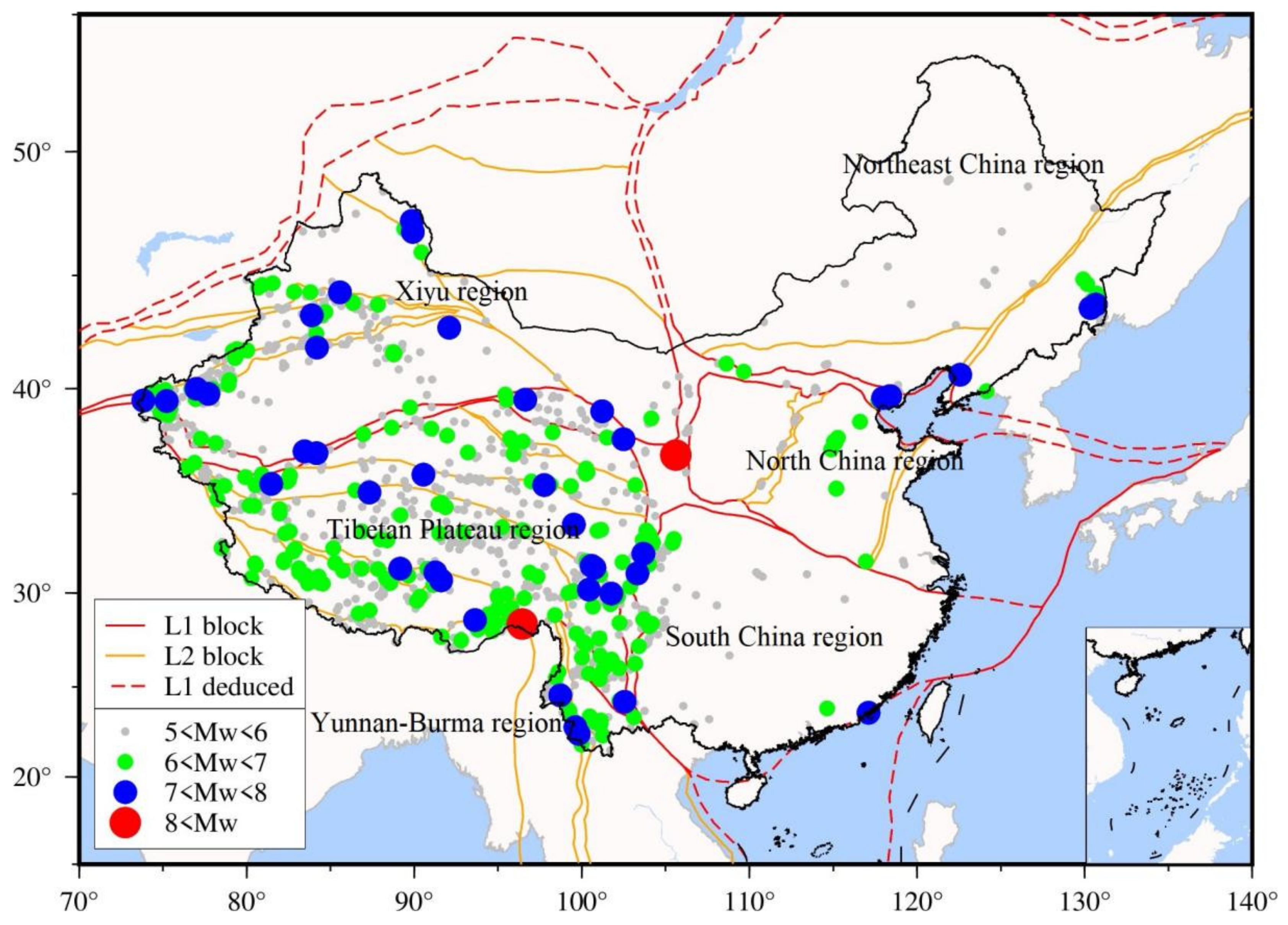Figure 1 shows the spatial distribution of earthquakes with Mw ≥ 5 in continental China in the past 100 years, which intuitively shows the characteristics of intense crustal movement in the western part of continental China. Most earthquakes are concentrated in the central Qinghai Tibet Plateau and surrounding areas.

With GNSS technology’s continuous progress and observation data accumulation, the space geodetic technology represented by GNSS has been widely used in the current research of crustal deformation monitoring in continental China because of its all-time observation, high spatial-temporal resolution, wide coverage, and high observation accuracy. At present, the monitoring of crustal movement and deformation in continental China has experienced a development process from small to large monitoring areas and from sparse to relatively dense stations [1]. Accordingly, the GNSS velocity field is also continuously improved and refined. Based on the early regional deformation monitoring data, Wang et al. (2001) published the results of the crustal movement velocity field in continental China, preliminarily showing the tectonic movement trend of the relatively stable Eurasian plate in continental China under the background of India Eurasian plate collision [3]. With the continuous updating and improvement of the crustal movement velocity field in continental China, some scholars have published a series of important achievements in studying crustal movement and deformation in continental China [4,5]. The results of the GNSS velocity field have also further promoted international research on major scientific issues such as the India–Eurasia collision and the deformation mechanism of the Qinghai Tibet Plateau [6,7,8]. In 2008, the implementation of CMONOC (Crustal Movement Observation Network of China) significantly improved the density of GNSS sites. Liang et al. (2013), Wang et al. (2017), Zheng et al. (2017), Rui et al. (2019), Bian et al. (2020) and Wu et al. (2020) published the results of the crustal movement velocity field or strain field of the Qinghai Tibet Plateau and its surrounding areas or the whole continental China by using the data of different periods [9,10,11,12,13,14], in which the vertical movement information given by Liang et al. (2013) revealed the overall uplift trend of the Qinghai Tibet Plateau relative to its northern stable block [9]. Wang and Shen (2020) published more intensive results of the crustal movement velocity field in continental China and its surrounding areas, to study the crustal deformation of continental China derived from GPS and its tectonic implications [2].

Extensive data collection, unified and rigorous processing of raw data, and correction of the co-seismic and post-seismic effects of large earthquakes are the three essential elements for the accuracy and reliability of the GNSS velocity field in continental China. The historical observations of CMONOC in the recent 20 years provide the necessary input data for the GNSS velocity field in continental China. It is also necessary to further reprocess and analyze the collected GNSS observations, and accurately build the co-seismic/post-seismic deformation model according to the major earthquake records of continental China in the recent 20 years.

With the updating of the GNSS precision processing model and algorithm, IGS will regularly reprocess historical GNSS observations to obtain unified and higher precision products and serve high-precision geoscience applications such as reference frames. IGS held its first GNSS observations reprocessing (repro1, http://acc.igs.org/reprocess.html, accessed on 1 May 2022) in 2012 and released the first GNSS reprocessing product based on ITRF2008 [15]. The second reprocessing (repro2, http://acc.igs.org/reprocess2.html, accessed on 1 May 2022) was held in 2014, and the corresponding GNSS reprocessing product based on ITRF2014 [16] was released. At present, the IGS third reprocessing campaign (repro3, http://acc.igs.org/reprocess3.html, accessed on 1 May 2022) aims to provide a time series of consistently reprocessed GNSS products covering the period from 1994 to 2020. The products are based on updated background models and processing methods. One of the main goals is to support the determination of the ITRF2020 [17,18] by providing daily coordinates for a global network of GNSS ground stations. Among them, IGS first processing is based on IERS2003 conventions [19], and the new absolute antenna phase center model (igs05.atx) is used to replace the long-term relative antenna phase center model, which can effectively eliminate the system error caused by the multi-path effect in the relative antenna phase center model, and the coordinate result quality is significantly improved [15,17]. The recommended error correction model is adopted for the IGS second reprocessing, for example, the antenna phase center model is igs08.atx file, IERS conventions are upgraded to the 2010 version [20]. Compared with the second reprocessing, the third reprocessing adopts some newly recommended models and conventions, including satellite and receiver antenna calibration, solar radiation pressure, earth reflectivity, polar tide, ocean tide, earth orientation parameters, time-varying gravity field, and other new methods. The accuracy of each reprocessing product will be significantly improved compared with the previous one, and the influence of untrue nonlinear site signals caused by imperfect models will be weakened [17].

To promote the dynamic research on the crustal tectonic activity and deformation process, and improve the reprocessing strategy of precise GNSS data in continental China, high-precision GNSS horizontal velocity field and plane crustal strain field, as well as the fine active block division model, this paper has carried out relevant research on the current crustal movement and tectonic deformation in continental China based on the GNSS observation data in the recent 20 years. Firstly, we have uniformly and strictly processed the GNSS observation data of continental China in the recent 20 years using the latest algorithm model of repro3. Furthermore, we refined GNSS horizontal velocity using the nonlinear site time series model and interpolated the grid velocity field of continental China. Then, based on the velocity results obtained from the above solution, the characteristics of the current crustal strain rate field in continental China are estimated and analyzed. Additionally, we further analyzed the relationship between the distribution of strong earthquakes and the characteristics of crustal deformation. In addition, we studied the block division using the GNSS horizontal velocity field in continental China and compared the characteristics and accuracy of the relative motion models of different blocks. Finally, we formulated some valuable conclusions.

2. GNSS Observation and Analysis

GNSS reprocessing can further weaken the influence of untrue nonlinear site signals caused by imperfect models, to improve the accuracy and reliability of the GNSS velocity field. In this section, we described the reprocess of two-decade GNSS observation to obtain a cleaner and more reliable GNSS coordinate time series. Then, the time series model considering nonlinear variations is refined to extract the GNSS velocity field, and the horizontal grid velocity field is obtained using Green’s function interpolation.

2.1. GNSS Observation Processing

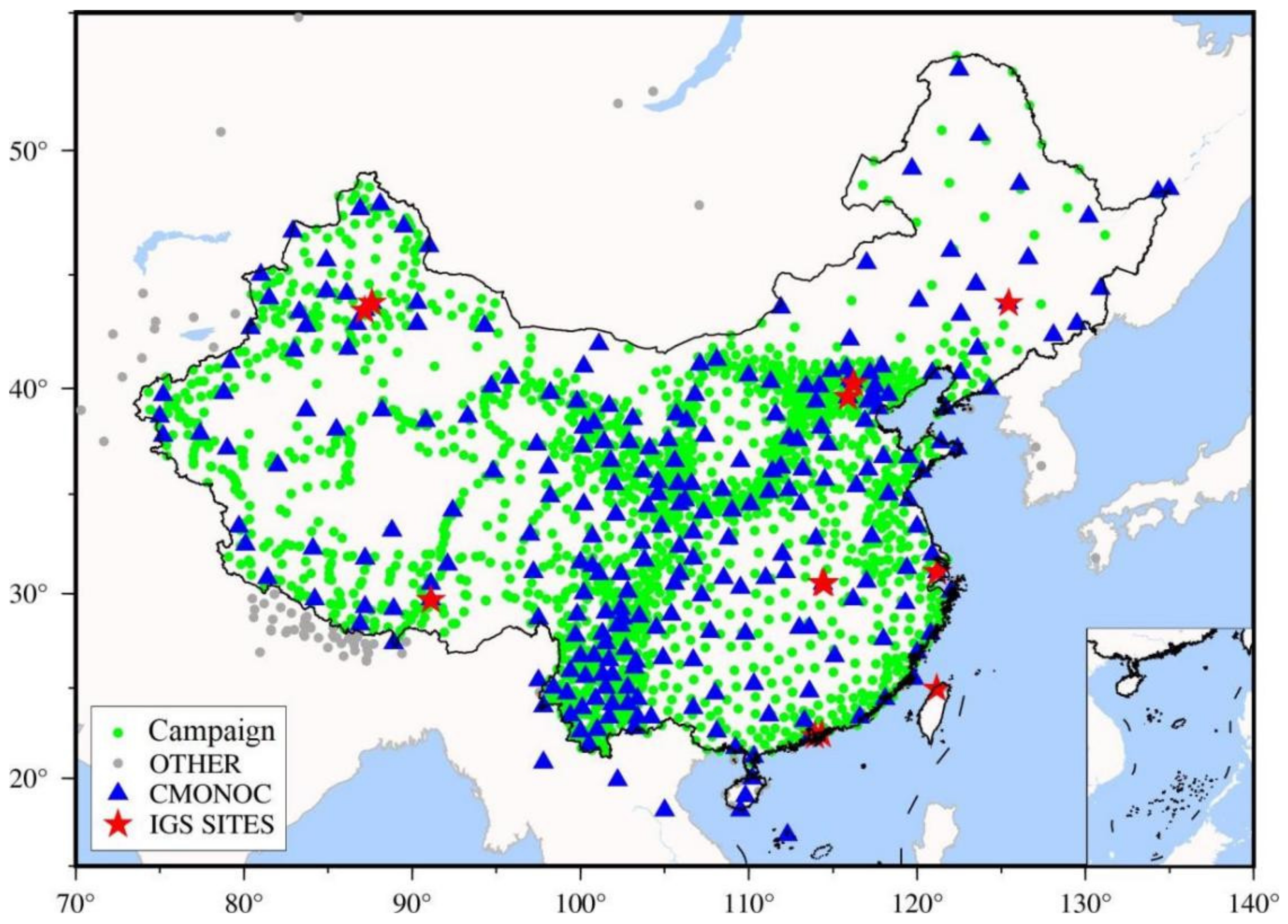
To ensure the accuracy and consistency of the GNSS coordinate solutions, we use the updated convention and processing settings of repro3 to reprocess the two-decade GNSS observations of continental China in an entirely consistent way. The offsets caused by receiver fault, antenna replacement, earthquake, and other factors can be detected using station logs, while the offsets caused by frame transformation, solution strategy, and model change need to be eliminated by data reprocessing. The basic input GNSS sites of this research are shown in Figure 2. The CMONOC comprises 260 continuous operation reference stations (daily observation) and more than 2000 regional stations (irregular observation). It has preliminarily realized the dynamic monitoring of the primary and secondary tectonic blocks, main active fault zones, and key seismic risk areas in continental China [1]. These GNSS stations have laid a foundation for describing the detailed characteristics of crustal movement in continental China. In addition, IGS stations around China and other continuous observation stations are collected.

At present, the accuracy of GNSS single-day static solution can reach mm level [21,22,23], whether a non-difference or double difference model is adopted. The commonly used GNSS precision solution software includes Bernese [24], GAMIT/GLOBK [25], Gipsy [26], PANDA [27,28], etc. The GAMIT/GLOBK software we selected is an open-source high-precision GNSS data processing software developed by the Massachusetts Institute of Technology (MIT) and Scripps Institute of Oceanography (SIO). Users can modify the source program according to their own needs. At present, the latest version of GAMIT/GLOBK is 10.7. GAMIT is based on the double-difference algorithm. Compared with the non-difference model, it can eliminate the impact of satellite and receiver clock errors and reduce atmospheric refraction errors and orbit errors [29,30]. GLOBK is a Kalman filter whose input information includes the estimation of station coordinates, earth rotation parameters, orbit parameters, and covariance matrix calculated by GAMIT. Then, the Kalman filter combines the GAMIT solutions in space and time. Finally, a reference frame consistent with a priori reference frame is established to obtain information on station coordinates, satellite orbit, earth rotation, and other parameters under this frame.

In addition to GNSS equipment replacement events, some major earthquakes can affect the position of surrounding stations (see Figure 1). Thus, we collected the significant earthquake events (Mw > 5) in continental China to determine the stations’ deformation due to earthquakes and model the co-seismic and post-seismic deformation. To ensure the quality of data solutions, the observation stations with observation periods of fewer than three years and sizeable coordinate time series residuals are excluded.

2.2. GNSS Velocity Field Refinement

In GNSS raw coordinate time series, it is usually necessary to consider the station trend term, (i.e., linear velocity, segmented velocity), periodic variation term (mainly affected by geophysical effects and false nonlinear errors), offset term caused by non-seismic factors, (i.e., equipment replacement, antenna height measurement error, phase center modeling error, other human and software errors) or seismic factors, post-seismic deformation term (usually in the form of exponential or logarithmic variation) and some unmodeled errors. Considering the above-mentioned factors, the GNSS time series model can be expressed explicitly as [31,32]:

$$\begin{gathered} X\left(t\right)=X_R+v\left(t-t_R\right)+{\displaystyle \sum }_{j=1}^{n_J}{b}_{j}H\left(t-t_j\right) \\ +{\displaystyle \sum }_{k=1}^{n_P}\left[s_{k}sin\left({\omega }_{k}t\right)+c_{k}cos\left({\omega }_{k}t\right)\right]+{\displaystyle \sum }_{m=1}^{n_T}{v}_k\left(t-t_m\right)H\left(t-t_m\right) \\ +{\displaystyle \sum }_{i=1}^{n_L}{A}_i^L\log \left(1+\frac{t-t_i^L}{{\tau }_i^L}\right)H\left(t-t_i^L\right)+{\displaystyle \sum }_{i=1}^{n_E}{A}_i^E\exp \left(1-e^{-\frac{t-t_i^E}{{\tau }_i^E}}\right)H\left(t-t_i^E\right)+\epsilon \end{gathered}$$

(1)

where $X\left(t\right)$ is the site coordinate at the epoch of $t$, $X_R$ is the site coordinate at the reference epoch of $t_R$, $v$ is the velocity of the station, $n_J=1,2,3\dots$ is the number of offsets, $t_j$ is the epoch of the offset $j$, ${\stackrel{\rightharpoonup }{b}}_j$ is the value of the offset $j$, $n_P=1,2\dots$ is the number of seasonal parameters, ${\omega }_k$ is the frequency of the $k$-th seasonal parameters, $s_k$ and $c_k$ are the amplitudes of the $k$-th seasonal parameters, $n_L=1,2,3\cdots$ and $n_E=1,2,3\cdots$ are the number of logarithmic and exponential models, $A_i^L\mathrm{and}{A}_i^E$ are the coefficient of logarithmic and exponential models, ${\tau }_i^L$ and ${\tau }_i^E$ are the seismic relaxation times in logarithmic and exponential models, $t_i^L$ and $t_i^E$ are the reference epoch in logarithmic and exponential models, $\epsilon$ is the observation noise.

Where H is expressed as:

$$H\left(t-t_j\right)=\left\{\begin{array}{c}0,t<t_j\\ \frac{1}{2},t=t_j\\ 1,t>t_j\end{array}\right.$$

(2)

The epoch of each event of the GNSS site can be available from the earthquake record, site log, detection algorithm, or visual inspection. The postseismic relaxation time is typically estimated separately by maximum likelihood methods so that the estimation of the remaining time series coefficients can be expressed as a linear inverse equation.

The seismic relaxation time is typically obtained from seismic products, or estimated separately by maximum likelihood methods so that estimation of the remaining GNSS coordinate time series parameters can be written as a linear equation:

$$\left\{\begin{array}{c}\mathit{y}=\mathit{B}\widehat{\mathit{X}}+\mathit{\epsilon }\\ {\mathit{E}}_{\epsilon }=\mathbf{0}\\ {\mathit{D}}_{\epsilon }={\sigma }_0^{2}c\end{array}\right.$$

(3)

where $\mathit{B}$ is the coefficient matrix and $\widehat{\mathit{X}}$ is the parameter vector to be fitted, $\widehat{\mathit{X}}={\left[X_{R}v\mathit{b}\mathit{s}\mathit{c}{\mathit{A}}^L{\mathit{A}}^E\right]}^T$, ${\mathit{E}}_{\epsilon }$ is the statistical mean value, ${\mathit{D}}_{\epsilon }$ is the statistical variance matrix, ${\mathit{C}}_{\epsilon }$ is the covariance matrix of observation errors, $\mathit{P}={\mathit{C}}_{\epsilon }{}^{-1}$ is the weight matrix, and ${\sigma }_0^2$ is an a priori variance factor.

According to the least square estimation (LSE) method, the estimation parameter vector is $\widehat{\mathit{X}}$ obtained by the Equation (4).

$$\widehat{\mathit{X}}={\left({\mathit{B}}^{\mathit{T}}\mathit{P}\mathit{B}\right)}^{-1}\left({\mathit{B}}^{\mathit{T}}\mathit{P}\mathit{L}\right)$$

(4)

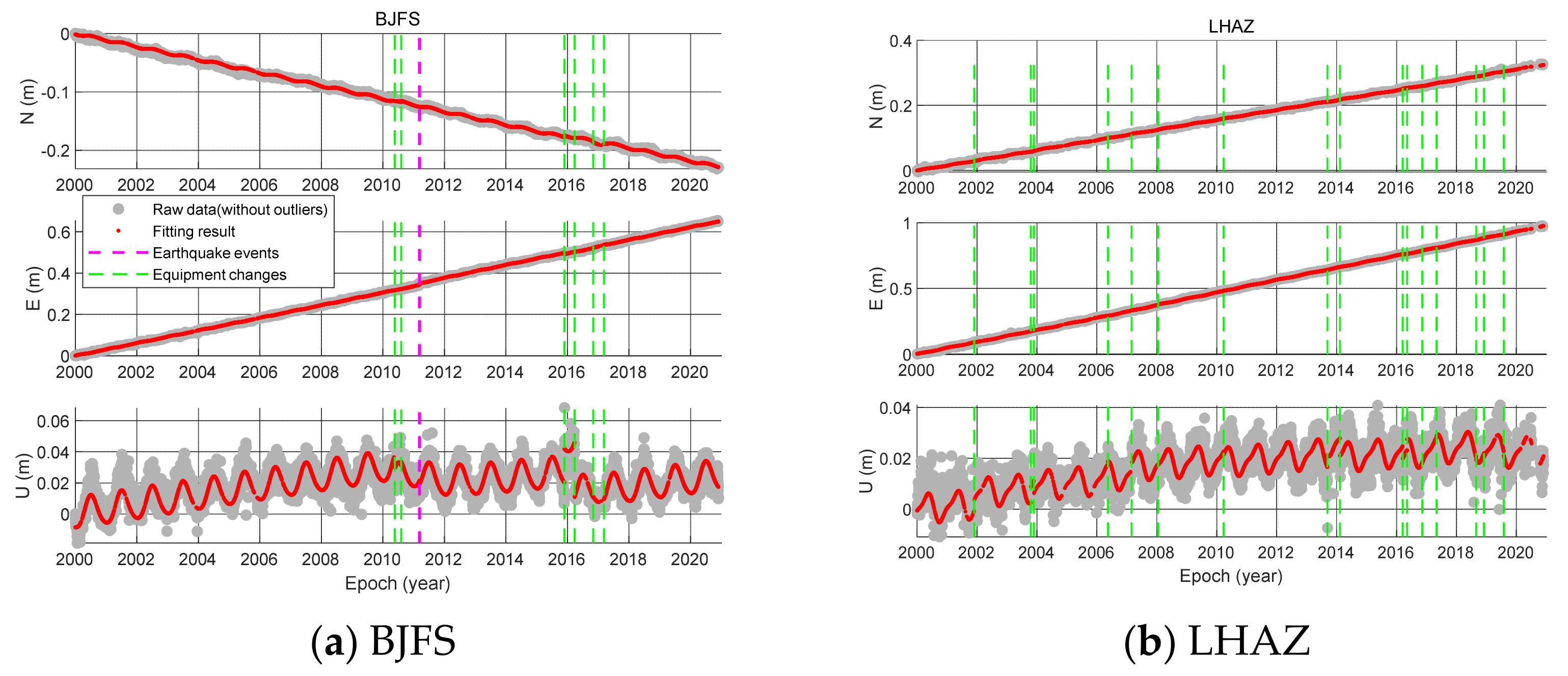
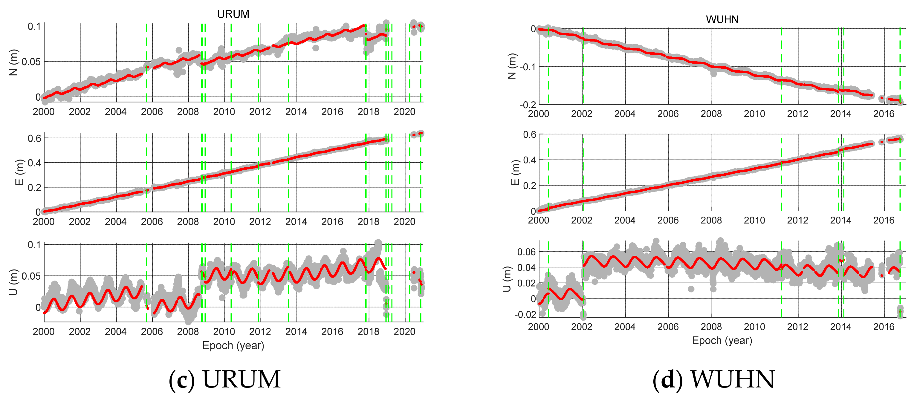
The fitting analysis is carried out based on the high-precision GNSS coordinate time series obtained in Section 2.1. We fully consider the velocity, annual and semi-annual period, offset, (i.e., equipment change and co-seismic deformation) and post-seismic deformation, to obtain the ITRF2014 GNSS velocity field through the robust least square fitting method. Taking BJFS, LHAZ, URUM, and WUHN as examples, Figure 3 shows the GNSS time series fitting process of the example station. In Figure 3, the gray dot is the raw data without very bad values (the horizontal coordinate precision is less than 10 cm, and the vertical precision is less than 20 cm), the red dot is the fitted value, the purple line is the epoch of earthquake, and the green line is the epoch of instrument replacement. It can be seen from the figure that the offsets in the sequence could seriously damage the internal characteristics of the series, which must be accurately detected and corrected. In addition, the seasonal deformation in the vertical direction is more obvious than that in the horizontal direction.

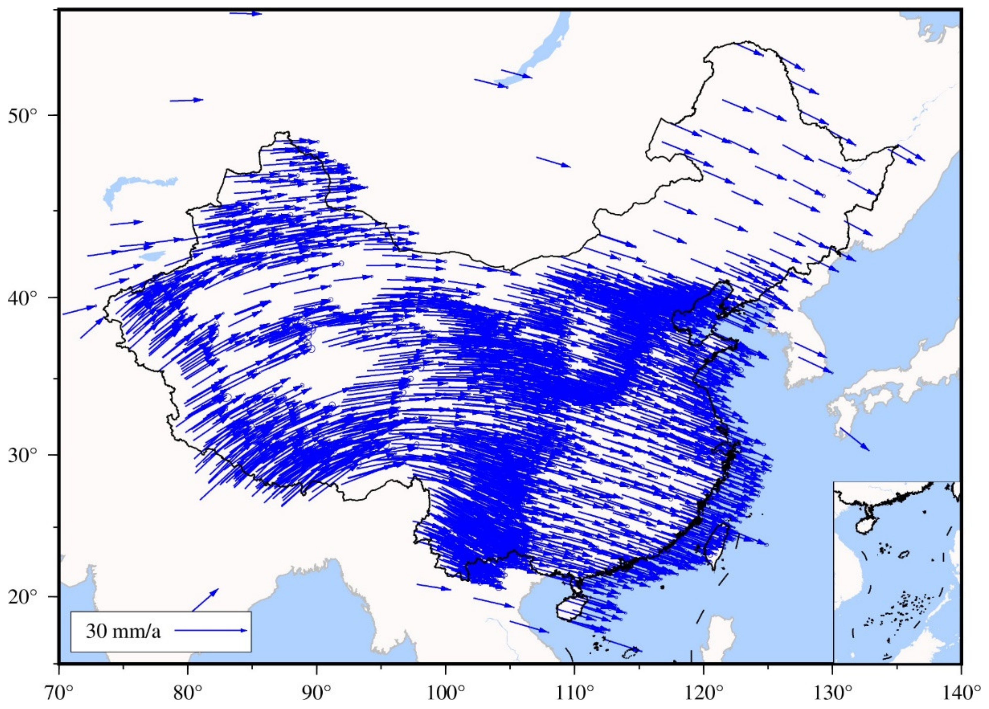
After analysis of the time series for all sites, we can obtain the ITRF2014 GNSS horizontal velocity field of continental China. As shown in Figure 4, there is a clockwise rotation movement from southwest to southeast in continental China, especially in the western region. The velocity field in the eastern region points from northwest to southeast.

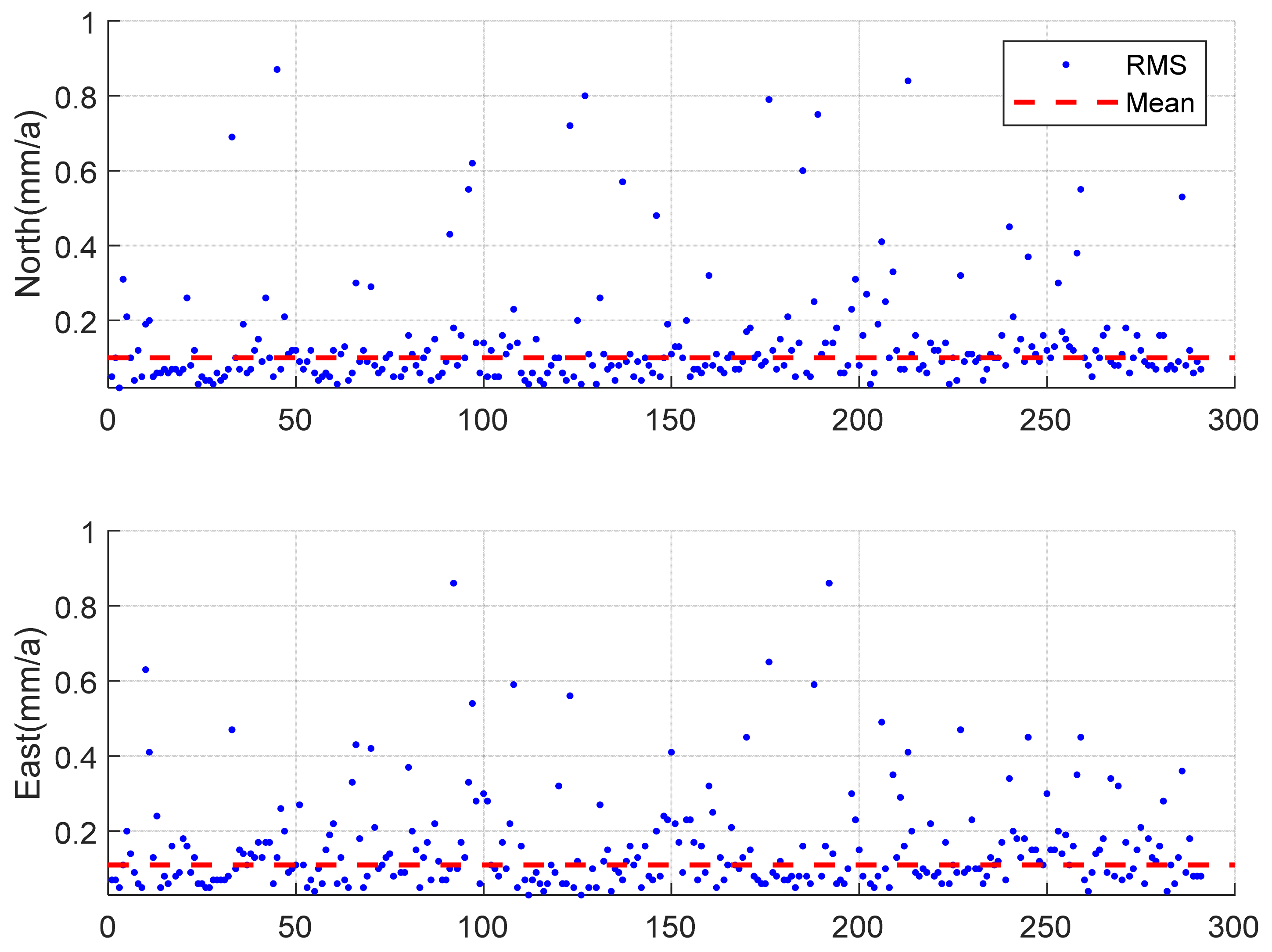
Figure 5 and

Table 1. The comparison of the horizontal velocity field in continental China.

Unit: mm/a	Continental China		East China		West China
	North	East	North	East	North	East
Median of velocity	−9.8	32.1	32.4	−10.7	31.2	5.6
Median of RMS	0.10	0.11	0.09	0.11	0.10	0.12

show the statistical accuracy of the horizontal velocity field in the east and west of continental China. The RMS of GNSS velocity in continental China is less than 1 mm/a as a whole, and the RMS of velocity in the north and east directions are 0.10 mm/a and 0.11 mm/a, respectively. In the east of China, the median velocity in the north and east directions are 32.4 mm/a and −10.7 mm/a, respectively. The median of RMS in the north and east directions are 0.09 mm/a and 0.11 mm/a, respectively. In the west of China, the median velocity in the north and east directions are 31.2 mm/a and 5.6 mm/a, respectively, as for the corresponding RMS values, 0.10 mm/a and 0.12 mm/a can be achieved in the north and east directions.

2.3. GNSS Velocity Field Gridding

The main purpose of velocity field interpolation is to obtain the continuous crustal strain rate field using the discrete GNSS station velocity. The new version of GMT [33] provides the gpsgridder [34] tool function module, which interpolates GNSS strains using Green’s functions for elastic deformation. Specifically, the gpsgridder grids two-dimensional vector data such as GNSS velocities using a coupled model based on two-dimensional elasticity. There are two main parameter adjustments in the gpsgridder method as follows: the first parameter is an appropriate minimum radius factor to prevent the singularity of Green’s function, and another is the value of Poisson’s ratio for interpolation. The degree of coupling can be tuned by adjusting the Poisson’s ratio such as incompressible (1.0), typical elastic (0.5), or even an unphysical value of −1 that removes the elastic coupling of vector interpolation. The interpolation of the two components on the grid of x is u(x) and v(x) [34,35]:

$$\{\begin{array}{l}u\left(\mathit{x}\right)={\sum }_{j=1}^{n}n{a}_{j}q\left(\mathit{x},{\mathit{x}}_j\right)+{ß}_{j}w\left(\mathit{x},{\mathit{x}}_j\right)\\ v\left(\mathit{x}\right)={\sum }_{j=1}^n{a}_{j}w\left(\mathit{x},{\mathit{x}}_j\right)+{ß}_{j}p\left(\mathit{x},{\mathit{x}}_j\right)\end{array}$$

(5)

where the three 2D elastic coupled Green’s functions are given by:

$$\left\{\begin{array}{c}q\left(\mathit{a},\mathit{b}\right)=\left(3-\nu \right)logr+\left(1+\nu \right)\frac{y^2}{r^2}\\ p\left(\mathit{a},\mathit{b}\right)=\left(3-\nu \right)logr+\left(1+\nu \right)\frac{x^2}{r^2}\\ w\left(\mathit{a},\mathit{b}\right)=-\left(1+\nu \right)\frac{xy}{r^2}\end{array}\right.$$

(6)

Here, $r$ is the radial distance between points $\mathit{a}$ and $\mathit{b}$. $x$ and $y$ are the components of that distance. The body forces ${\alpha }_j$ and ${\beta }_j$ are obtained by evaluating the solution at the data locations and inverting the square linear system that results, $\nu$ is Poisson’s ratio.

The Euler vector mentioned above is usually used to describe the long-term rotational motion characteristics of plates. If the Earth is approximated as a regular sphere, the center of mass of the Earth remains unchanged, and the block on the Earth’s surface is regarded as a rigid body. According to Euler’s theorem, the motion of the block on the Earth’s surface can be regarded as the fixed axis rotation passing through the center of the Earth, which satisfies the Equation (7):

$$\mathit{V}=\mathsf{\Omega }\times \mathit{R}$$

(7)

where $\mathit{V}$ is the station velocity in a block, $\mathsf{\Omega }$ is the Euler vector of the plate, and $\mathit{R}$ is the position vector of the station. It can be rewritten into a formula convenient for calculation:

$$\left[\begin{array}{c}{V}_e\\ V_n\end{array}\right]=R\left[\begin{array}{ccc}-cos\lambda sin\phi & -sin\lambda sin\phi & cos\phi \\ sin\lambda & -cos\lambda & 0\end{array}\right]\left[\begin{array}{c}{\mathsf{\Omega }}_x\\ {\mathsf{\Omega }}_y\\ {\mathsf{\Omega }}_z\end{array}\right]$$

(8)

where $V_e$ and $V_n$ are the horizontal velocity of a station; $R$ is the average radius of the Earth, about 6,371,393 m. $\lambda$ and $\phi$ are the geodetic latitude and longitude of the station, ${\mathsf{\Omega }}_x$, ${\mathsf{\Omega }}_y$ and ${\mathsf{\Omega }}_z$ are the three components of the Euler vector.

${\mathsf{\Omega }}_x$, ${\mathsf{\Omega }}_y$ and ${\mathsf{\Omega }}_z$ in the Cartesian coordinate system are expressed as ${\mathsf{\Omega }}_{\lambda }$, ${\mathsf{\Omega }}_{\phi }$ and ${\mathsf{\Omega }}_{\omega }$ in spherical coordinates. Where ${\mathsf{\Omega }}_{\lambda }$ and ${\mathsf{\Omega }}_{\phi }$ are Eulerian latitude and longitude, and ${\mathsf{\Omega }}_{\omega }$ is rotational angular velocity. The corresponding relationship is:

$$\left\{\begin{array}{c}{\mathsf{\Omega }}_x=\omega ·cos{\mathsf{\Omega }}_{\phi }·cos{\mathsf{\Omega }}_{\lambda }\\ {\mathsf{\Omega }}_y=\omega ·cos{\mathsf{\Omega }}_{\phi }·sin{\mathsf{\Omega }}_{\lambda }\\ {\mathsf{\Omega }}_z=\omega ·sin{\mathsf{\Omega }}_{\phi }\end{array}\right.$$

(9)

$$\left\{\begin{array}{l}{\mathsf{\Omega }}_{\lambda }=arctan\left({\mathsf{\Omega }}_y/{\mathsf{\Omega }}_x\right)\\ {\mathsf{\Omega }}_{\phi }=arcsin\left({\mathsf{\Omega }}_z/\omega \right)\\ {\mathsf{\Omega }}_{\omega }=\sqrt{{\mathsf{\Omega }}_x^2+{\mathsf{\Omega }}_y^2+{\mathsf{\Omega }}_z^2}\end{array}\right.$$

(10)

where the value range of $\lambda$ is [−90, 90], and the value range of $\phi$ is [−180, 180].

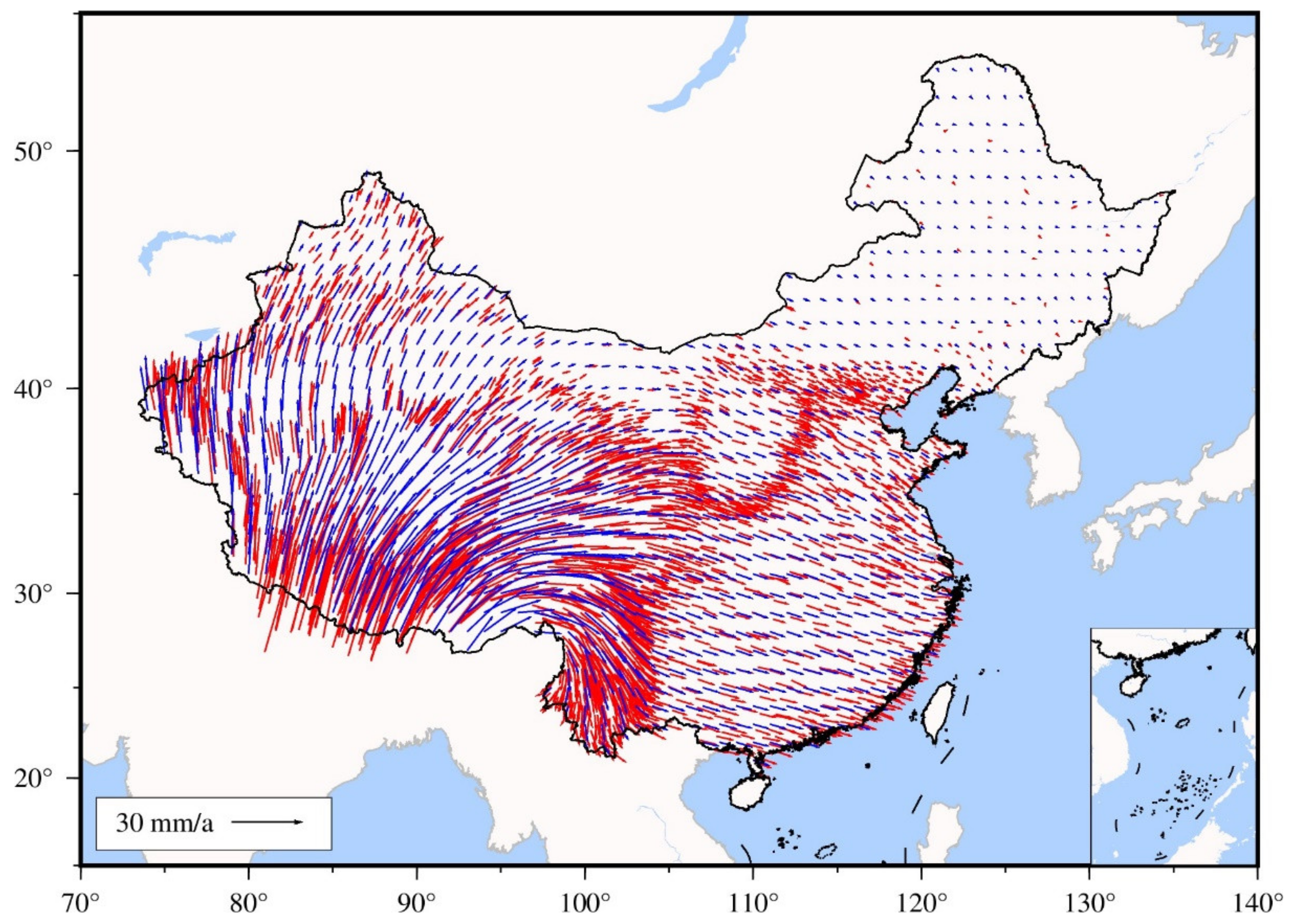
According to Euler parameter transformation, the ITRF2014 velocities are transformed into the velocities under the Eurasian reference frame. Based on the GNSS horizontal velocity field in continental China, we attempt to use the gpsgridder method to interpolate the horizontal grid velocity field in continental China. In the interpolation process, the data outside the research areas and the velocity with an error larger than 1 mm/a are eliminated. In addition, the velocity with an error larger than twice the median error and the ones with a significant deviation between the velocity direction and the overall motion trend is also eliminated.

The gpsgridder method of GMT6 has two main parameter adjustments. One parameter is a minimum radius factor to keep Green’s functions from being singular. After some trial and error, we find that the minimum radius of 16 km performs the best overall fitted result, which also roughly corresponds to the mean spacing of all GNSS sites in the study area [36]. The other parameter is Poisson’s ratio used for the velocity interpolation. We test a range of −1 (fully decoupled), 0.5 (elastic), and 1.0 (incompressible), while different results have little difference. Thus, we use the recommended value of Poisson’s ratio of 0.5 [13,34]. In the experiment, we set the Poisson’s ratio of 0.5 and the minimum radius of 16 km, and finally obtained the horizontal grid velocity field (1° × 1°) of continental China, as shown in Figure 6. The red arrow is raw velocity, and the blue arrow is interpolation velocity.

3. GNSS Crustal Strain Rate

GNSS velocity field can directly reflect the characteristics of crustal movement in the study area under a certain reference frame, and its spatial distribution characteristics will vary with the change of datum. While the crustal strain field is not limited by datum, and it can reflect the dynamic mechanism of crustal deformation. This section estimates the GNSS horizontal crustal strain rate field in continental China using the GNSS horizontal velocity field of more than 2000 sites from the above solution to analyze the characteristics of the current crustal strain rate field in continental China.

3.1. Estimation of Crustal Strain Rate Tensor

Due to the low accuracy of GNSS vertical velocity, the study of GNSS crustal deformation is usually focused on the analysis of horizontal ground strain rate. The parameters of horizontal ground strain rate are estimated by the horizontal gradient of the GNSS velocity field. Based on the infinitesimal strain theory, the discrete GNSS velocity can be expressed as [37]:

$$V_i=U_i+\frac{\partial V_i}{\partial x_j}d{x}_j=U_i+e_{ij}d{x}_j$$

(11)

where $V_i$ is the component of the velocity vector in the direction of $i$, $U_i$ is the velocity component in the direction of the origin position of $i$, $d{x}_j$ is the component in the direction of $j$, $e_{ij}$ is the velocity gradient. According to the theory of tensor analysis, any second-order tensor can be decomposed into the sum of a symmetric tensor and an antisymmetric tensor, which is expressed as:

$$e_{ij}=\frac{e_{ij}+e_{ji}}{2}+\frac{e_{ij}-e_{ji}}{2}={\tau }_{ij}+{\omega }_{ij}$$

(12)

where ${\tau }_{ij}$ is strain tensor, ${\omega }_{ij}$ is rotation tensor. The maximum principal strain tensor ${\tau }_1$ and the minimum principal strain tensor ${\tau }_2$ are expressed as:

$$\left\{\begin{array}{c}{\tau }_1=\frac{1}{2}\left({\tau }_{ii}+{\tau }_{jj}\right)+\frac{1}{2}\sqrt{{\left({\tau }_{ii}-{\tau }_{jj}\right)}^2+4{\tau }_{ij}^2}\\ {\tau }_2=\frac{1}{2}\left({\tau }_{ii}+{\tau }_{jj}\right)-\frac{1}{2}\sqrt{{\left({\tau }_{ii}-{\tau }_{jj}\right)}^2+4{\tau }_{ij}^2}\end{array}\right.$$

(13)

The direction angle $\theta$ of the maximum principal strain tensor ${\tau }_1$ is expressed as:

$$\theta =\frac{1}{2}{\tan }^{-1}\left(\frac{2{\tau }_{ij}}{{\tau }_{ii}-{\tau }_{jj}}\right)$$

(14)

The maximum shear strain tensor ${\gamma }_{max}$ is expressed as:

$${\gamma }_{max}=\frac{1}{2}\sqrt{{\left({\tau }_{ii}-{\tau }_{jj}\right)}^2+4{\tau }_{ij}^2}=\frac{{\tau }_1-{\tau }_2}{2}$$

(15)

The surface expansion tensor $\mathsf{\Delta }$ is expressed as:

$$\mathsf{\Delta }={\tau }_{ii}+{\tau }_{jj}={\tau }_1+{\tau }_2$$

(16)

The second strain invariant $E_2$ is expressed as:

$$E_2=\sqrt[2]{{\tau }_{ii}^2+{\tau }_{jj}^2+2{\tau }_{ij}^2}=\sqrt[2]{{\tau }_1^2+{\tau }_2^2}$$

(17)

3.2. Characteristic Analysis of Crustal Strain

The principal strain rate field of continental China can be estimated using the horizontal grid velocity field (1° × 1°). The overall pattern of tectonic deformation in continental China in the past two decades is shown in Figure 7. The principal strain rate in West China is much higher than that in East China. Among them, the principal strain rate in the west is large, and the strain distribution is complex, indicating that the crustal deformation in this area is intense and the geological tectonic movement is more complex. The high-strain areas in continental China are mainly located in the Qinghai Tibet Plateau and Tianshan Mountains. The principal compressive strain rates of the Himalayas and Tianshan orogenic belts are perpendicular to the orogenic belt trend, and the other principal strain rate is much lower than the principal compressive strain rate, revealing the northward pushing of the Indian plate. In contrast, the total amount of principal strain rates in the east is small. The principal strain rates of several active blocks in the east are less than 5 nstrain/year, and the principal strain rate field has no significant regional distribution characteristics.

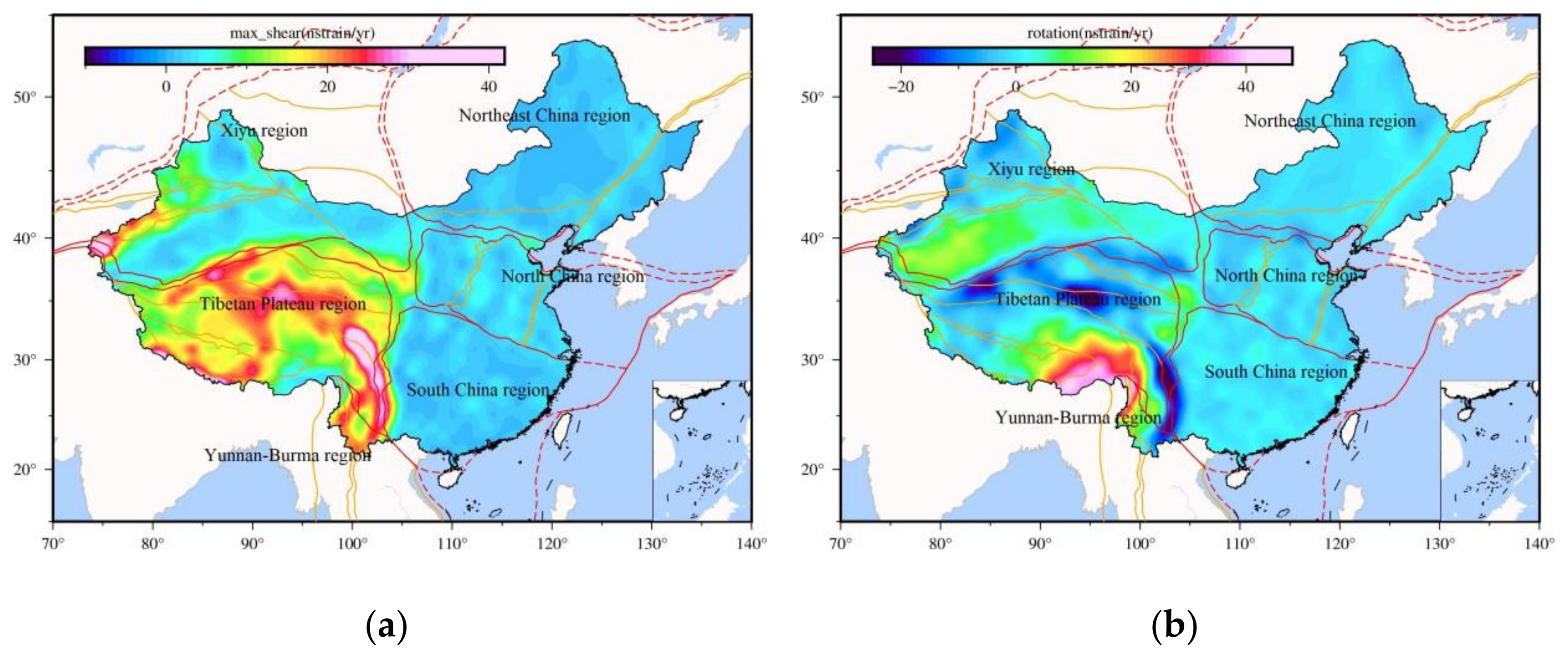
To better reflect the regional crustal deformation characteristics of continental China, the distribution characteristics of other GNSS horizontal strain rate fields in continental China, such as the maximum shear strain rate field (Figure 8a), rotation rate field (Figure 8b), surface expansion rate field (Figure 8c), and the second strain invariant field (Figure 8d) are estimated.

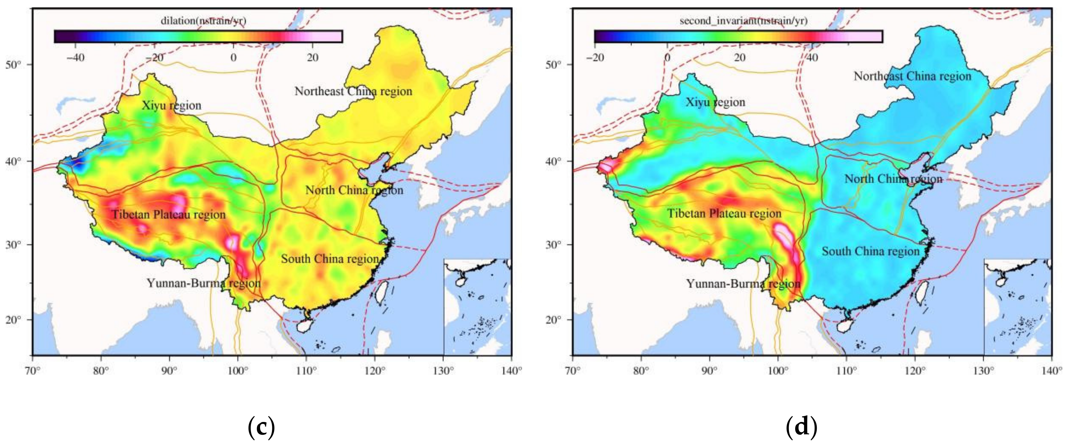
The maximum shear strain rate, rotation rate, surface expansion rate, and the second strain invariant in continental China show regional distribution characteristics similar to the principal strain rate field, that is, the strain degree in the west is much more intense than that in the east. Compared with the strain rate distribution characteristics dominated by block movement in the east, the strain rate field in the western Qinghai Tibet Plateau and its surrounding areas has more intense and complex distribution characteristics. The analysis results are basically consistent with the continuum deformation field of continental China published by Wang et al. 2020 [2]. The difference is that Wang Ming’s results are larger in the western region, so the deformation analysis in the western edge region is more specific. In addition to the maximum shear strain, dilatation rate, and rotation rate, we also add the analysis of the distribution characteristics of the surface expansion and second strain invariant. Therefore, the existing strain field model of the Chinese mainland is further updated and improved.

For the maximum shear strain rate, the maximum shear strain rate in the region is located at the junction of the Anninghe Zemuhe fault zone and the Xiaojiang fault zone on the southeast edge of the Qinghai Tibet Plateau. The distribution of the maximum shear strain rate near the main fault zones in the western region shows intense shear deformation near these fault zones. For the regional rotation rate, the maximum rotation rate in the region is located in the eastern Himalayan tectonic zone, and the position of the minimum rotation rate value coincides with the maximum shear strain rate. For the surface expansion rate, the surface compressibility of the Longmenshan fault zone, the north section of Xiaojiang fault zone, Karakoram fault zone, Himalayan main boundary thrust zone, and South Tianshan fault zone is the most significant, and the surface compressibility near the Himalayan main boundary thrust zone is the largest. The surface expansion rate of the south section of the Xiaojiang fault zone and the north section of the Honghe fault zone is the most significant, and the surface expansion rate near the north section of the Honghe fault zone is the largest. The second strain invariant has the basically same spatial distribution as the maximum shear strain field, indicating that the areas with intense crustal deformation in the Qinghai Tibet Plateau and its surrounding areas are accompanied by significant shear deformation. To sum up, the magnitude of the principal strain rate of the Qinghai Tibet Plateau and its surrounding areas is much larger than that of eastern continental China, and there is a stronger relative crustal movement in the region.

3.3. Relationship between Crustal Deformation and Strong Earthquake

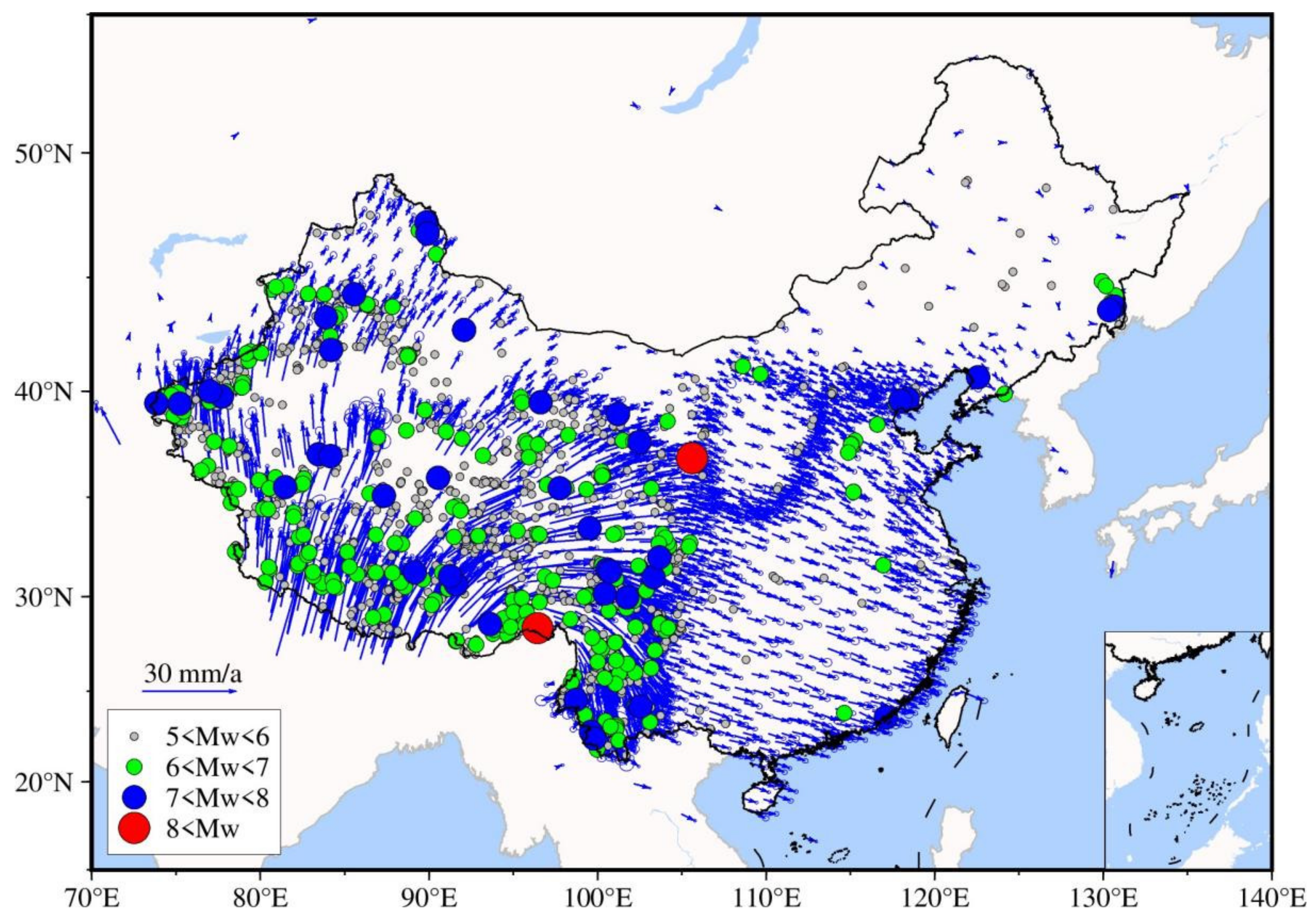
We collect historical earthquake records (Mw ≥ 5) in continental China during the period of 1900 to 2020 (seismic data from https://earthquake.usgs.gov, accessed on 1 May 2022). The characteristics of seismicity in the Chinese mainland show that the frequency of earthquakes is relatively high. The earthquakes above magnitude 8 are all distributed in western China. Most of the magnitude 7 earthquakes were concentrated in the western region, and several magnitude 7 earthquakes occurred in the eastern region. Strong earthquakes are mainly concentrated near faults, active blocks, and block boundary zones in the Chinese mainland.

As can be seen from Figure 9, there is a strong correlation between the spatial location of strong earthquakes and the direction and size of the GNSS horizontal velocity field, that is, strong earthquakes will occur where the magnitude and direction of GNSS velocity change dramatically. For example, the size and direction of the GNSS velocity field in the Tarim, Qinghai Tibet Plateau, and Sichuan Yunnan regions have changed significantly, and these regions are the areas where strong earthquakes occur frequently.

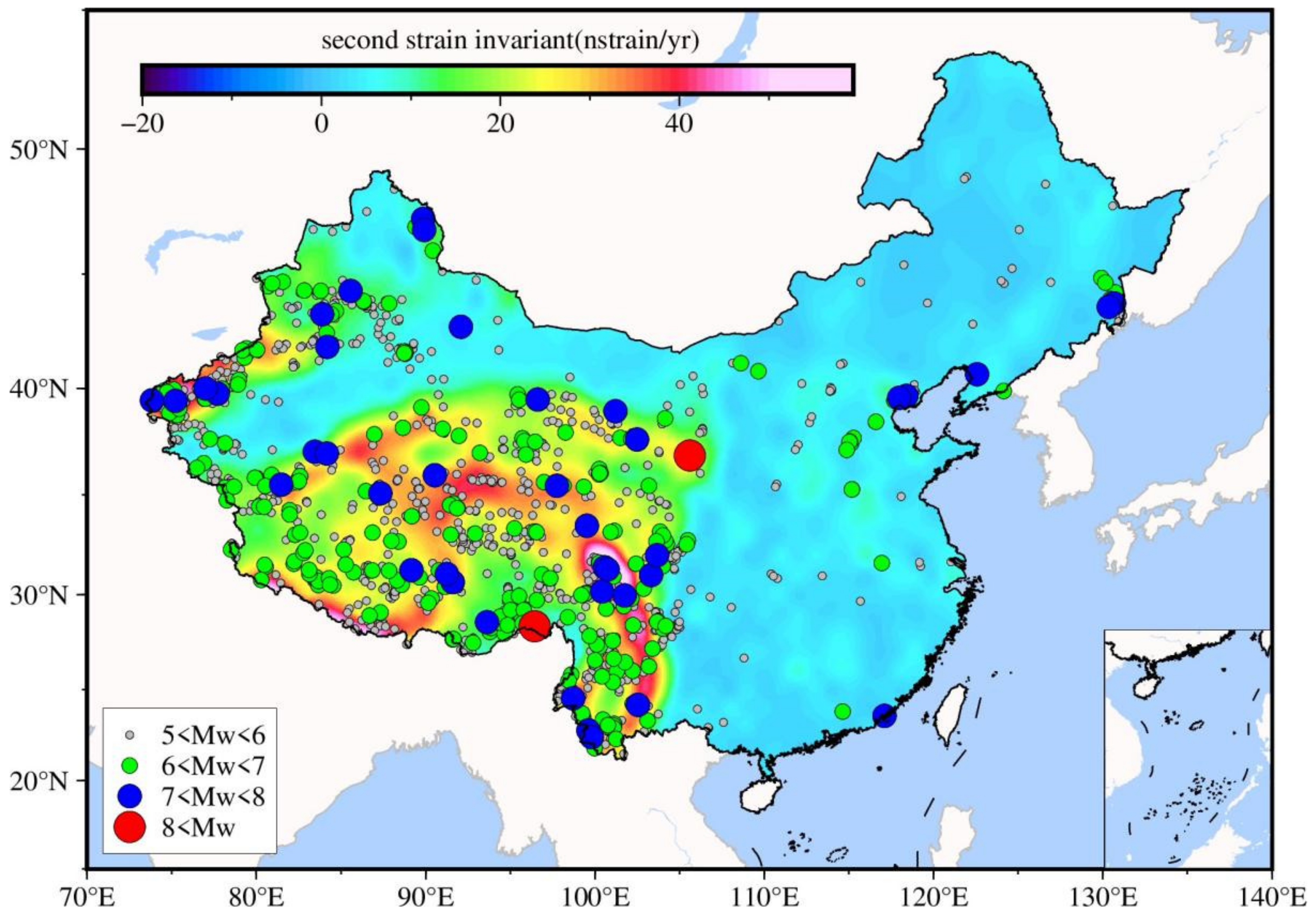
Figure 10 shows the relationship between a strong earthquake and the second strain invariant field in the Chinese mainland. Similarly, we find that there is a strong correlation between the distribution of strong earthquakes and the second strain invariant field, that is, most strong earthquakes are concentrated in yellow and red areas where the second strain invariant is greater than 20 nstrain/year. It can be seen that the second strain rate invariance of the Tianshan, Qinghai, Tibet Plateau, and Sichuan–Yunnan regions is large, and the second strain rate invariance changes greatly. The range of the second strain rate in Sichuan Yunnan, Qinghai Tibet Plateau, and Tianshan region are 5~40, 10~60, and 10~45 nstrain/year respectively. In fact, strong earthquakes occur widely in the Qinghai, Tibet Plateau, Sichuan Yunnan, and Tianshan regions, while there are relatively few strong earthquake activities in other regions. From this, we can infer that the occurrence of strong earthquakes is closely related to the magnitude and change rate of the second strain rate invariant field.

According to the relationship between the above strong earthquake distribution and GNSS velocity field and the second strain invariant field, we can draw the following conclusions. First, strong earthquakes occur when the magnitude and direction of the GNSS velocity field change greatly. The change of velocity field is caused by the mutual compression of crustal structures of different active blocks. The stronger the regional velocity change, the higher the frequency of strong earthquakes. Secondly, strong earthquakes usually occur in areas with large strain rates and large changes in strain rates. All strong earthquakes with Mw ≥ 7 are distributed in the region where the second strain rate invariance is greater than 20 nstrain/year.

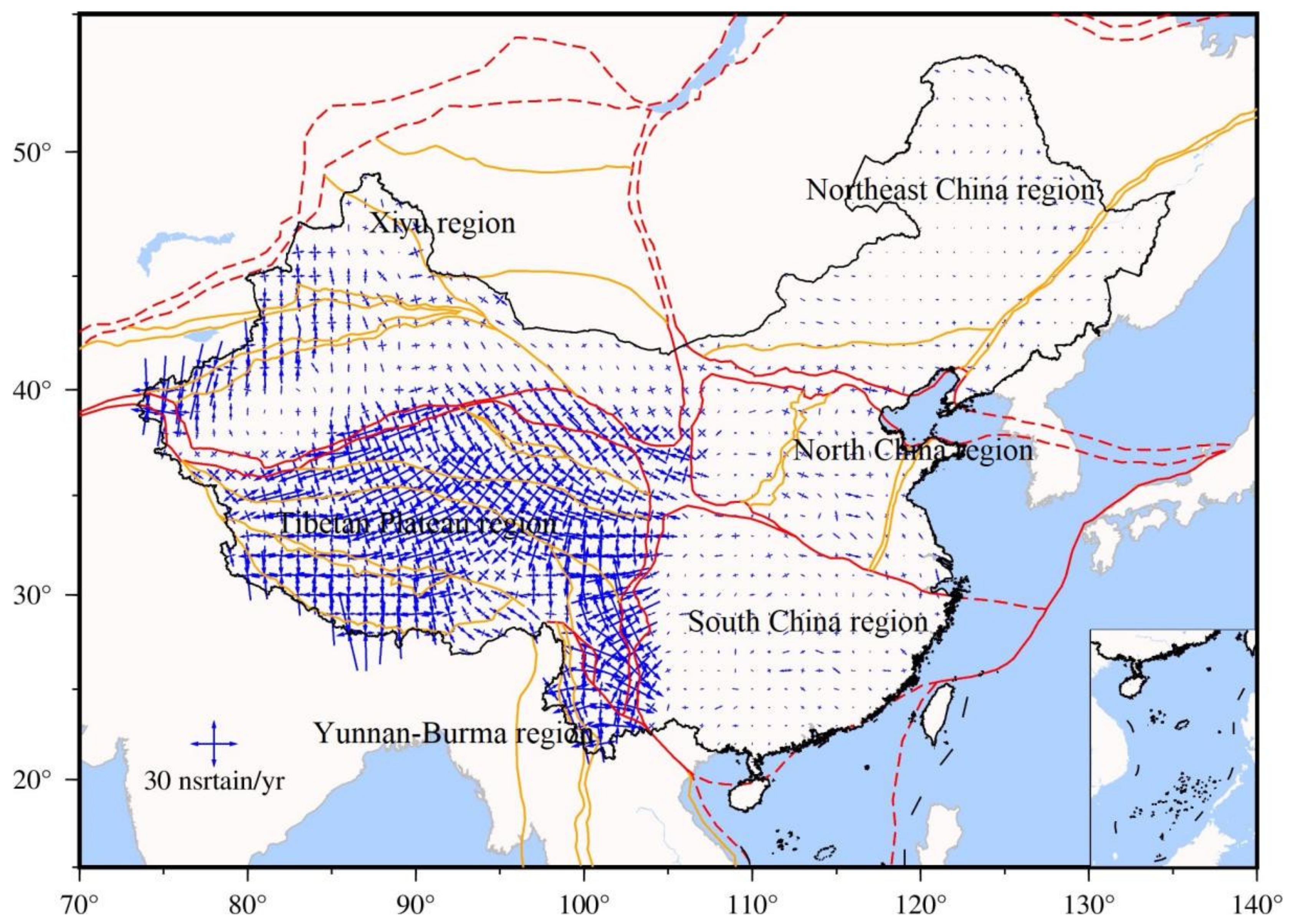
4. Block Division Using GNSS Velocity Field

For a GNSS network with a small area, the HAC method or K-means clustering method can effectively realize block division based on the GNSS velocity field [38,39,40,41,42]. Among them, the K-means algorithm is an unsupervised classification model that is widely used, simple, and effective. However, due to the randomness of the initial point selection of the algorithm, it may lead to wrong classification results. Therefore, we adopt the improved K-means++ [43] algorithm. Generally, the crustal deformation mechanism in a small area is relatively simple, and the block can be divided by the velocity of the station, so the classical clustering method can be used. The deformation mechanism of a large area is relatively complex, so more attributes must be considered to improve the accuracy of block division. In addition, for a GNSS network with a large area, the K-means++ method only considers the size of the GNSS velocity vector and ignores the direction of the velocity vector. Thus, the clustering of the GNSS velocity field based on the K-means++ method maybe not accurately reflect the actual characteristics of the spherical crustal deformation field. It is necessary to improve the clustering analysis of the GNSS velocity field on the Earth’s surface. The rotational motion characteristics of the rigid motion of a block on Earth’s surface can be expressed by the Euler vector. So, for the cluster analysis of the GNSS velocity field with a large area, the Euler vector features of active blocks can be used as additional constraints to further improve the accuracy of block division.

4.1. Improved GNSS Velocity Clustering Method

Without any prior assumptions, we use the improved K-means++ clustering analysis method to divide continental China into blocks with the high-precision GNSS horizontal velocity result. The algorithm of block division using the improved K-means method can be described as follows [44]:

(1)

Select center: randomly select a velocity vector as the initial clustering center. Firstly, calculate the quadratic distance between each station and the current existing cluster center. Then, estimate the probability that each station is selected as the next cluster center. Finally, cycle to select the next cluster center. Repeat the previous step until N cluster centers are selected.

(2)

Start cluster: take N cluster centers as a reference, calculate the distance between the velocity vector of other stations and the reference point one by one, take it as the consideration index of their similarity, and assign the velocity vector of the station to the data cluster where the reference point with the smallest distance is located.

(3)

Iterative cluster: recalculate the cluster center for each data cluster. Repeat steps (2) and (3) until the position of the cluster center does not change.

(4)

Correct cluster: based on the cluster results obtained in step (3) calculate the relative velocity of the station in each cluster block to the corresponding Euler pole. Suppose the station velocity relative to the Euler pole of other blocks is less than its own block, and the difference value exceeds the error limit level. In that case, the station will be reassigned to the block with the minimum velocity. Then, every site will be reassigned to a more appropriate block. In the case of station redistribution, repeat the above steps until the velocity of all stations is no longer redistributed.

The block Euler vector value is estimated according to the least square principle. Rewrite the error equation according to Formula (4) as follows:

$$\mathit{V}=\mathit{B}\widehat{\mathit{X}}-\mathit{L}$$

(18)

where $\mathit{V}$ is the observation correction, $\mathit{B}=R\left[\begin{array}{ccc}-cos\lambda sin\phi & -sin\lambda sin\phi & cos\phi \\ sin\lambda & -cos\lambda & 0\end{array}\right]$, L = $\left[\begin{array}{c}{V}_e\\ V_n\end{array}\right]$, $\widehat{\mathit{X}}=\left[\begin{array}{c}{\mathsf{\Omega }}_x\\ {\mathsf{\Omega }}_y\\ {\mathsf{\Omega }}_z\end{array}\right]$.

4.2. Results of Block Division of Continental China

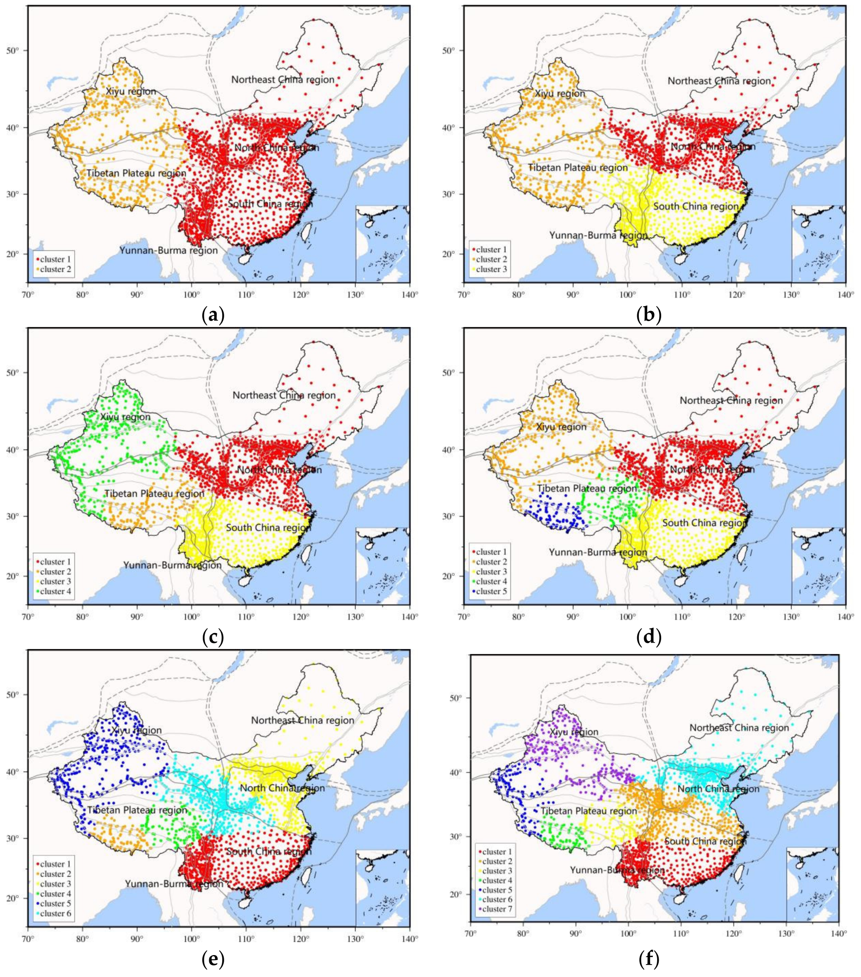
Since the number of blocks divided in the Chinese mainland is unknown, we need to try different cluster numbers with 2–7 to further analyze and discuss the results of active block division. The block division results based on the improved K-means++ cluster analysis method using GNSS horizontal velocity field in continental China are shown in Figure 11. It can be seen from the figure that different block division results are relatively consistent with the existing accurate block division results [45]. More detailed block division results are as follows:

When N = 2, due to the obvious difference in GNSS velocity between the east and the west of continental China, the continent is divided into two large blocks. When N = 3, the east continental block is further divided into two blocks, namely the northeast block and the southeast block. The northeast block contains the existing North China block. When N = 4, the west continental block is further divided into two blocks, namely the Tibet block and Qinghai Tibet block. When N = 5, the Qinghai Tibet block is further divided into two blocks, of which the Alisa block is separated from the north. When N = 6, the junction of five first-class blocks on the mainland is divided into one part, which may be due to the unobvious difference in velocity at the junction. When N = 7, the South China block in the east of the continent is further divided into two sub-blocks.

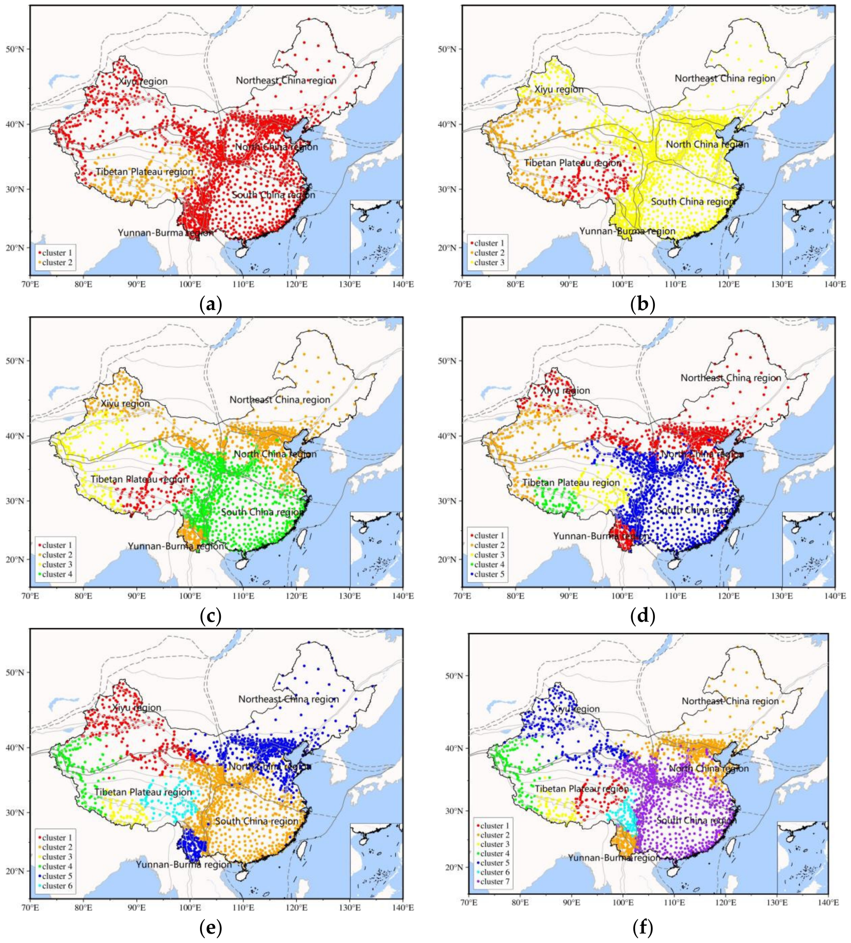
To verify the accuracy and reliability of the improved K-means++ method, Figure 12 gives the results of block division with the K-means++ method. Similarly, we try different cluster numbers with 2–7 to analyze and discuss the results of active block division. Obviously, the division result of these blocks using the K-means++ method is not consistent with the law of crustal activity. For example, in the following different block division results, there is a phenomenon that stations not in the same region are divided into unified blocks. However, in fact, this result is unreasonable. It is because the K-means++ method only considers the GNSS velocity’s size and ignores the direction of the velocity and other attribute information that the GNSS stations in different regions are divided into unified blocks.

The block division results based on the improved K-means++ cluster method using GNSS horizontal velocity in continental China coincide with the existing block [45] and have certain reliability and credibility. With the increase in the number of clusters, especially the west region is divided in more detail. Due to the great difference in crustal activity characteristics between the east and west regions, we will try to divide the east and west regions of continental China, respectively, in future research.

The traditional geological data determination method [45] requires a detailed analysis of hundreds of years of geological data to divide blocks, and the process is complex. In contrast, the improved K-means++ clustering method can obtain accurate block division results only based on the accurate GNSS horizontal velocity field in the past two decades, and it is simpler to use. Compared with the K-means++ method, the improved K-means++ clustering method uses Euler vector features of active blocks to further improve the accuracy of block division, and it takes into account the size and direction attributes of GNSS velocity at the same time. Thus, the improved K-means++ clustering method is more accurate and reliable.

4.3. Refinement of Block Euler Vector Motion

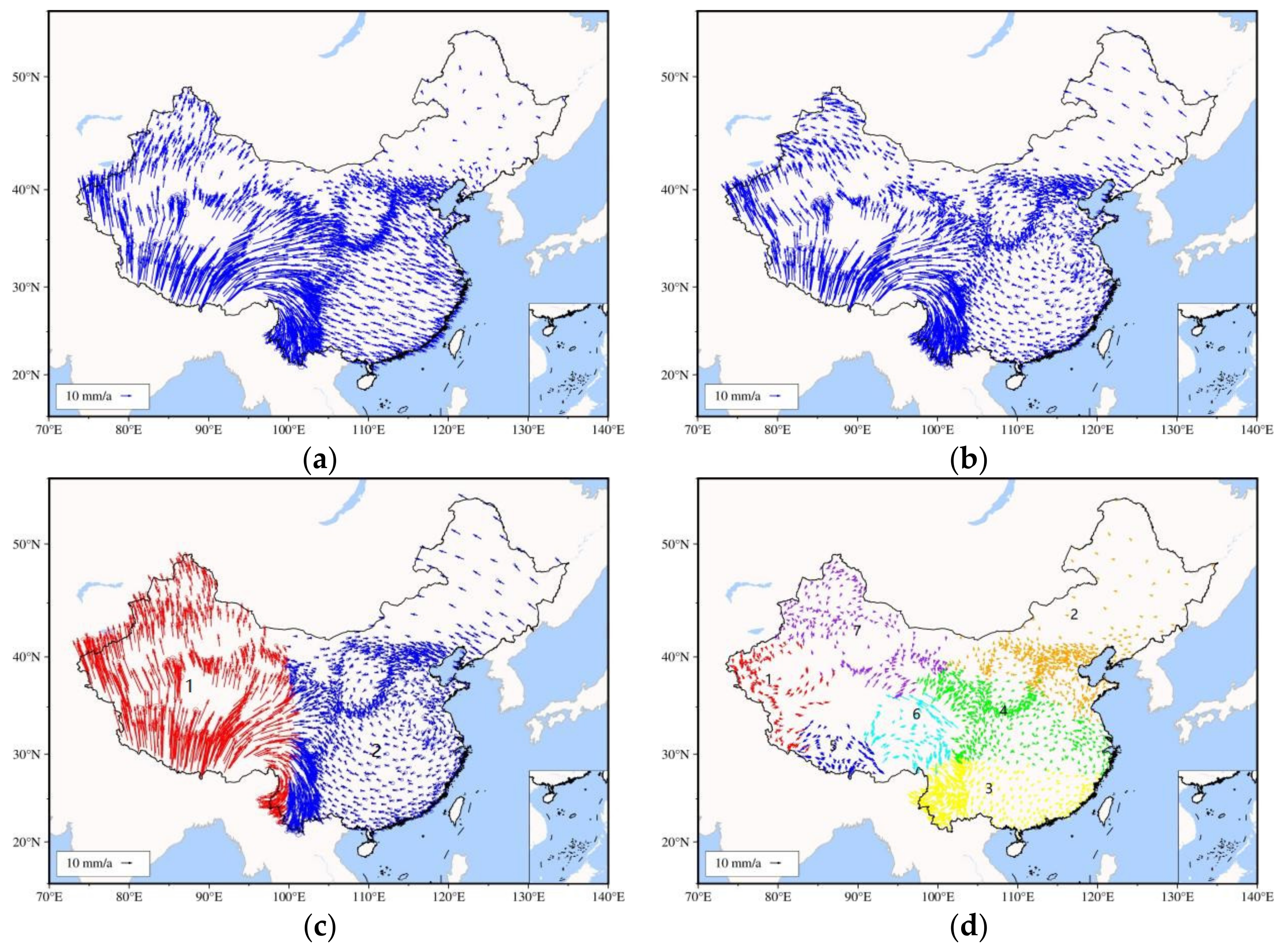
To improve the accuracy of the horizontal relative velocity field model of continental China and describe its local movement characteristics more accurately, we have constructed the relative movement model of the Eurasian plate and the relative motion model of the whole plate based on the Euler vector. Based on the above block division results of GNSS velocity field cluster analysis in continental China, we further construct the relative movement model of blocks in continental China (the number of blocks is 2 and 7, respectively). The specific method is to substitute the horizontal velocity, longitude, and latitude of the station and the Euler parameter value in

Table 2. Euler parameters and accuracy statistics of different block models in continental China.

Block	Index	${\mathsf{\Omega }}_{\mathbf{x}}$	${\mathsf{\Omega }}_{\mathbf{y}}$	${\mathsf{\Omega }}_{\mathbf{z}}$	${\mathsf{\Omega }}_{\mathbf{\omega }}$	Sve	Svn	Msve	Msvn
		10−3 rad/Ma				mm/a
Eurasian	1	0.4121	−2.5744	3.7331	4.5534	5.60	9.65	5.60	9.65
China 1	1	−0.0170	−4.2669	3.4931	5.5144	5.83	8.49	5.83	8.49
China 2	1	−0.9523	−2.0238	5.0876	5.5575	6.51	9.40	5.80	7.37
	2	1.2046	−4.3371	3.6922	5.8218	5.12	5.35
China 7	1	2.1372	−3.6553	3.2059	5.3110	2.45	3.00	2.60	2.65
	2	−0.9841	−1.9506	4.9608	5.4206	0.94	0.88
	3	−2.0908	−0.0258	5.9182	6.2767	3.90	3.01
	4	−0.1701	−3.9485	3.9843	5.6119	1.60	1.87
	5	2.9764	−4.7682	4.6384	7.2876	3.24	3.30
	6	1.5021	−15.6942	−1.2248	15.8134	4.10	4.18
	7	0.4443	−3.4167	3.5738	4.9641	1.90	2.35

into Formula (3), and subtract it from the known velocity to obtain the GNSS relative velocity, as shown in Figure 13.

(1)

Compared with the Eurasian plate, West China is moving towards the northeast as a whole, and East China is moving towards the east, and the relative velocity field is large. The accuracy of the velocity field in the west is lower than that in the east.

(2)

The movement trends of China block 1 and China block 2 are the same. There are apparent regional motion characteristics in the east. The region with the most intense motion is mainly concentrated in the boundary of the Qinghai Tibet active block, and the eastern region takes the Bohai Rim region as the center, showing a reverse time needle vortex motion trend. The southwest region takes the Qinghai Tibet region as the center and rotates clockwise. The northwest region is bounded by the boundary between Junggar and Tianshan Mountains, moving to the southwest and northwest.

(3)

The relative movement model of China block 7 can significantly weaken the movement trend in local areas. Taking 105°E as the boundary, the tectonic movement in West China is more intense. Except for a few stations in the eastern part, the residual velocity of other stations is small. The relative velocity of each sub-block is small and less than 5 mm/a, and the RMS of mean velocity is about 2.6 mm/a. Among them, the relative velocity of Qinghai Tibet and Sichuan Yunnan in the western region is large, which is caused by the violent internal tectonic movement.

Table 2 shows the accuracy of Euler parameters and relative velocities of different block models in continental China. Among the four models, the Euler vector of the Eurasian block is taken from the reference [46]: ${\mathsf{\Omega }}_{\lambda }$ = −99.10°, ${\mathsf{\Omega }}_{\phi }$ = 55.07°, ${\mathsf{\Omega }}_{\omega }$ = 0.261 × 10⁻³°/Ma. The Euler parameters of other different blocks are calculated by LSE based on the station velocity in the block. In order to ensure the accuracy and reliability of the results, iterative least squares are used for calculation, and the triple RMS rule is used to eliminate outliers in each iteration. Euler parameters ${\mathsf{\Omega }}_x$, ${\mathsf{\Omega }}_y$, ${\mathsf{\Omega }}_z$ and ${\mathsf{\Omega }}_{\lambda }$, ${\mathsf{\Omega }}_{\phi }$, ${\mathsf{\Omega }}_{\omega }$ can be converted to each other through Formulas (9) and (10).

It can be seen from Table 2 that the RMS of the four models is: Eurasian plate < China block 1 < China block 2 < China block 7. Among them, the accuracy of the Eurasian plate model is the lowest, and the RMS of relative velocity in the east and north directions are 5.60 and 9.65 mm/a. The models of China block 1 and China block 2 are the same, the accuracy of China block 7 has been significantly improved, and the mean RMS of relative velocity in the east and north directions are 2.60 and 2.65 mm/a. The mean RMS of the horizontal velocity of the first three models is more than 5 mm/a, and the mean RMS of each block in China block 7 is less than 5 mm/a, of which the largest is the 6th sub-block, and the relative RMS in the east and north directions are 4.10 and 4.18 mm/a. It should be noted that the sixth sub-block of China block 7 is located in the Qinghai Tibet Plateau. Its crustal activity is intense, and the local rotation changes significantly, with the rotation rate reaching 15 × 10⁻³ rad/Ma.

5. Conclusions

We used more observations (2260+ sites), longer time (20 years), and updated standard (Repro3) to obtain GNSS velocity field in continental China, and finely described crustal deformation and active block with the gpsgridder and improved K-means++ approaches. The research results show that:

(1)

GNSS reprocessing based on repro3 can obtain a cleaner and more reliable GNSS coordinate time series. The GNSS velocity field in continental China is refined using the nonlinear time series model. The accuracy of the GNSS horizontal velocity field is better than 1.0 mm/a, and the RMS mean of velocity is 0.1 mm/a. Compared with ITRF2014, the interior of continental China presents a clockwise rotation movement from southwest to southeast. It is proven by repeated experiments that the minimum radius is set to 16 and Poisson’s ratio is set to 0.5, when the gpsgridder method is used to interpolate the GNSS horizontal velocity field in continental China.

(2)

By analyzing the crustal strain characteristics of continental China, it can be concluded that the strain in West China is much more intense than that in the east. The total principal strain rate in East China is small, the value of the principal strain rate is less than 5 nstrain/year, and the principal strain rate field has no significant regional distribution characteristics. The high-strain areas in continental China are mainly located in the Qinghai Tibet Plateau and Tianshan Mountains. The principal compressive strain rates of the Himalayas and Tianshan orogenic belts are perpendicular to the orogenic belt trend, and the other principal strain rate is much lower than the principal compressive strain rate, revealing the northward pushing of the Indian plate. In addition, by analyzing the relationship between earthquake distribution and crustal deformation characteristics, it can be concluded that most strong earthquakes in the Chinese mainland occurred on active blocks and their boundary faults with large changes in the GNSS velocity field and strain field.

(3)

The improved K-means++ clustering analysis method divides the active blocks in continental China. The results show that the block results coincide with the existing block division results. As the number of clusters increases, the western region is divided in more detail. When the number of blocks reaches seven, the division results of active blocks in continental China are more in line with the actual situation. Compared with other methods, the improved K-means++ clustering method is simpler, and it uses Euler vector features of active blocks to further improve the accuracy of block division, and it takes into account the size and direction attributes of GNSS velocity at the same time.

(4)

The relative movement model of China block 7 can significantly weaken the movement trend in local areas. Taking 105°E as the boundary, the tectonic movement in West China is more intense. Except for a few sites, the residual velocity of other stations is small in the east. Among the four different block models of continental China, the accuracy of the Eurasian block is the lowest (the RMS of relative velocity in the east and north directions are 5.60 and 9.65 mm/a), followed by China block 1 and China block 2, and the accuracy of continental block 7 is the highest (the RMS mean of relative velocity in the east and north directions are 2.60 and 2.65 mm/a). The RMS of the velocity of each block in the continental block 7 is less than 5 mm/a, of which the largest is the sixth sub-block (the RMS in the east and north directions are 4.10 and 4.18 mm/a, and the rotation rate reaches 15 × 10⁻³ rad/Ma). The results also verify the feasibility of block division based on the GNSS velocity field in continental China.

In general, the emergence and development of GNSS technology in the 1990s significantly promoted the research of tectonic movement and deformation monitoring into a new stage. With over 30 years of research, horizontal tectonic movement and main deformation characteristics in continental China have been clear, and the tectonic deformation in most areas has been accurately quantified. In the future, it is necessary to intensify the continuous GNSS observation further to obtain the three-dimensional tectonic movement information and its evolution characteristics with time. At the same time, it is necessary to strengthen the integration of GNSS and different geodetic technologies, and interdisciplinary research.