Mapping Paddy Rice in Complex Landscapes with Landsat Time Series Data and Superpixel-Based Deep Learning Method

Abstract

The spatial pattern and temporal variation in paddy rice areas captured by remote sensing imagery provide an effective way of performing crop management and developing suitable agricultural policies. However, fragmented and scattered rice paddies due to undulating and varied topography, and the availability and quality of remote sensing images (e.g., frequent cloud coverage) pose significant challenges to accurate long-term rice mapping, especially for traditional pixel and phenological methods in subtropical monsoon regions. This study proposed a superpixel and deep-learning-based time series method to analyze Landsat time series data for paddy rice classification in complex landscape regions. First, a superpixel segmentation map was generated using a dynamic-time-warping-based simple non-iterative clustering algorithm with preprocessed spectral indices (SIs) time series data. Second, the SI images were overlaid onto the superpixel map to construct mean SIs time series for each superpixel. Third, a multivariate long short-term memory full convolution neural network (MLSTM-FCN) classifier was employed to learn time series features of rice paddies to produce accurate paddy rice maps. The method was evaluated using Landsat imagery from 2000 to 2020 in Cengong County, Guizhou Province, China. Results indicate that the superpixel MLSTM-FCN achieved a high performance with an overall accuracy varying from 0.9547 to 0.9721, which presents an 0.17–1.23% improvement compared to the random forest method. This study showed that combining spectral, spatial, and temporal features with deep learning methods can generate accurate paddy rice maps in complex landscape regions.

1. Introduction

As one of the most important staple crops in China, rice provides food for about 65% of Chinese people [1]. Paddy rice agriculture is a crucial component in national and global food security. However, pests and diseases continue to have detrimental effects on rice production [2,3]. In addition, maintaining the rice planting area is a critical challenge for global food security [4]. Accelerating urbanization and the “Grain for Green” project may create continual pressure on the rice planting area [5]. Furthermore, paddy rice agriculture also plays an essential role in water use and climate change. Rice agriculture requires a considerable amount of water [6]. The total water consumption of rice irrigation around the world accounts for about a quarter to one-third of global freshwater usage [7,8]. Rice paddies are an important source of methane emissions, contributing approximately 11% of total anthropogenic methane emissions [9]. Methane emissions from rice paddies significantly influence climate change by accelerating global warming [10]. Consequently, the spatial distribution of paddy rice is valuable information for agriculture management, and understanding and assessing pests and diseases, food security, climate change, and water usage at regional, national, and global scales [11]. Compared to conventional agricultural sample surveys for rice sowing areas, spaceborne remote sensing is recognized as a highly efficient and reliable approach for obtaining timely and accurate paddy rice cultivation areas [8,12].

Spaceborne remote sensing techniques have been used to map paddy rice planting areas for serval decades in Asian countries [13,14,15,16]. The agronomic practice of flooding paddy rice fields and transplanting rice seedlings, followed by a rice growth period, provides a unique reflectance or backscatter temporal profiles and mechanisms to differentiate paddy rice from other vegetations [17,18]. In previous studies, Synthetic Aperture Radar (SAR) images, such as Sentinel-1, RADARSAT, and PALSAR, have been particularly suitable for mapping paddy rice in the cloudy regions since SAR images are less affected by weather conditions, such as cloud and rain [19,20,21,22]. Nevertheless, the acquisition capability of SAR systems is usually not as good as that of optical sensors, and SAR images have not been used for long-term paddy rice mapping [8,23].

Many efforts have been made to map paddy rice using optical remote sensing products using the Moderate-Resolution Imaging Spectroradiometer (MODIS) or Landsat programs [6]. These studies have employed several techniques for temporal classification of spectral reflectance data or spectral indices (SIs), such as the Normalized Difference Vegetation Index (NDVI), the Enhanced Vegetation Index (EVI), the Land Surface Water Index (LSWI), the Normalized Difference Snow Index (NDSI), and others [16,24,25,26,27,28,29,30]. Because of the daily revisit frequency of the MODIS satellite, it has become an important optical data source for phenology-based paddy rice mapping [14,27]. However, paddy rice fields are often patchy and fragmented, and MODIS data are insufficient for mapping paddy rice due to their coarse spatial resolution (i.e., 250 m and 500 m) [6,20]. Compared with MODIS images, Landsat images have a finer spatial resolution, and they have also been widely used in paddy rice mapping [13,26,29,30]. Moreover, the free access to Landsat archive data from the past forty years (i.e., 1972 to the present) offers unique opportunities to document long-term dynamics in paddy rice planting areas. Dong et al. [26] generated the extent of paddy rice cover in northeast China over the past three decades at five-year intervals based on Landsat images, which provided direct evidence for continuously expanding paddy rice planting areas. In general, previous studies have verified that optical remote sensing methods can be used to map the extent of paddy rice cover at the regional scale. A primary complicating factor is acquiring enough cloud-free images in the rice-growing season to capture paddy rice phenology, given frequent and persistent cloud coverage during the rice-growing season as induced by monsoons [15,31]. Therefore, studies are needed to differentiate the paddy rice fields from Landsat time series images with relatively low temporal frequency and irregular data availability.

Dong and Xiao [6] reviewed the evolution of remote-sensing-based paddy rice mapping methods from the 1980s to 2015. Their study emphasized the critical role played by phenological phases in paddy rice mapping. Phenology-based methods can quantitatively recognize the key phenological periods and have been proven to be robust in identifying paddy rice regions [6,18]. The most representative and widely used phenology-based method is the transplanting-based algorithm [25,26,31,32]. This algorithm distinguishes paddy rice based on the relationship between the NDVI (or EVI) and LSWI during the paddy rice transplant phase (i.e., the period of rice plants–water–soil mixing) and specifically whether LSWI values are temporarily close to or greater than NDVI (or EVI) values during this period [25,33]. Recently, machine learning algorithms have been applied to differentiate paddy rice from remote sensing images, such as the ISODATA classifier [34], random forest (RF) classifiers [21,22,35], support vector machines (SVM) [36,37], and deep learning [17,30,38,39,40]. Studies based on deep learning methods have improved performance and shown great promise. For example, Zhang et al. [30] found that a convolutional neural network (CNN) could identify paddy rice in phenological variable images which derived from a time series Landsat-like NDVI with an overall accuracy (OA) of 97%; the accuracy was 6% and 8% greater than the OA of SVM and RF classifiers. However, these studies rely on the reliable and unique phenological variables of different extents of land cover, which remains challenging in complex regions with variable topography, landscape composition, and configuration [16,41,42], such as rice planting areas in South and Southwest China. In such regions, the undulating terrain, non-uniform phenology, and small, irregular, and fragmented rice paddies generally mixed with other croplands lead to difficulties in rice mapping using phenological variables due to the spatial proximity and spectral similarity to other land types [42,43,44]. In addition, the salt-and-pepper effect is another issue in using per-pixel classification for complex landscapes [16].

Identifying paddy rice could be regarded as a multivariate time series (MTS) classification task with two classes: rice and non-rice. With the recent vigorous development of deep learning, ensemble deep learning models have been developed to accommodate the time series classification problem without heavy preprocessing or feature engineering. For example, Karim et al. [45] proposed the multivariate long short-term memory (LSTM) full convolution neural network (FCN) (MLSTM-FCN) classification method. The proposed MLSTM-FCN model was tested on 35 datasets and achieved strong performances with most of them. Therefore, the MLSTM-FCN was employed to identify the paddy rice in the Landsat SIs time series in this study. Due to object-based classification producing better results than per-pixel methods [12], a superpixel segmentation algorithm was employed to generate superpixels as objects.

The goal of this study was to use ensemble deep learning models with Landsat data to map annual paddy rice coverage. This method could generate precise rice paddy maps with 30 m-spatial-resolution images for complex regions. The specific objectives of the study were to (1) evaluate the potential of Landsat time series images for mapping rice paddy in complex regions; (2) compare the performance of the per-pixel-based and superpixel-based MLSTM-FCN classifier and RF classifier in mapping paddy rice with SIs time series; and (3) map the temporal variation in paddy rice using time series Landsat images.

The contribution of this study is two-fold. The first contribution integrates agronomic domain knowledge with deep learning methods to generate accurate paddy rice maps, and this approach could be extended to other crop studies as well. On the other hand, the superpixel approach proposed in this paper could be employed to accommodate various spatial-temporal analytics in agriculture, which offers a baseline for decision making in agriculture management.

2. Materials and Methods

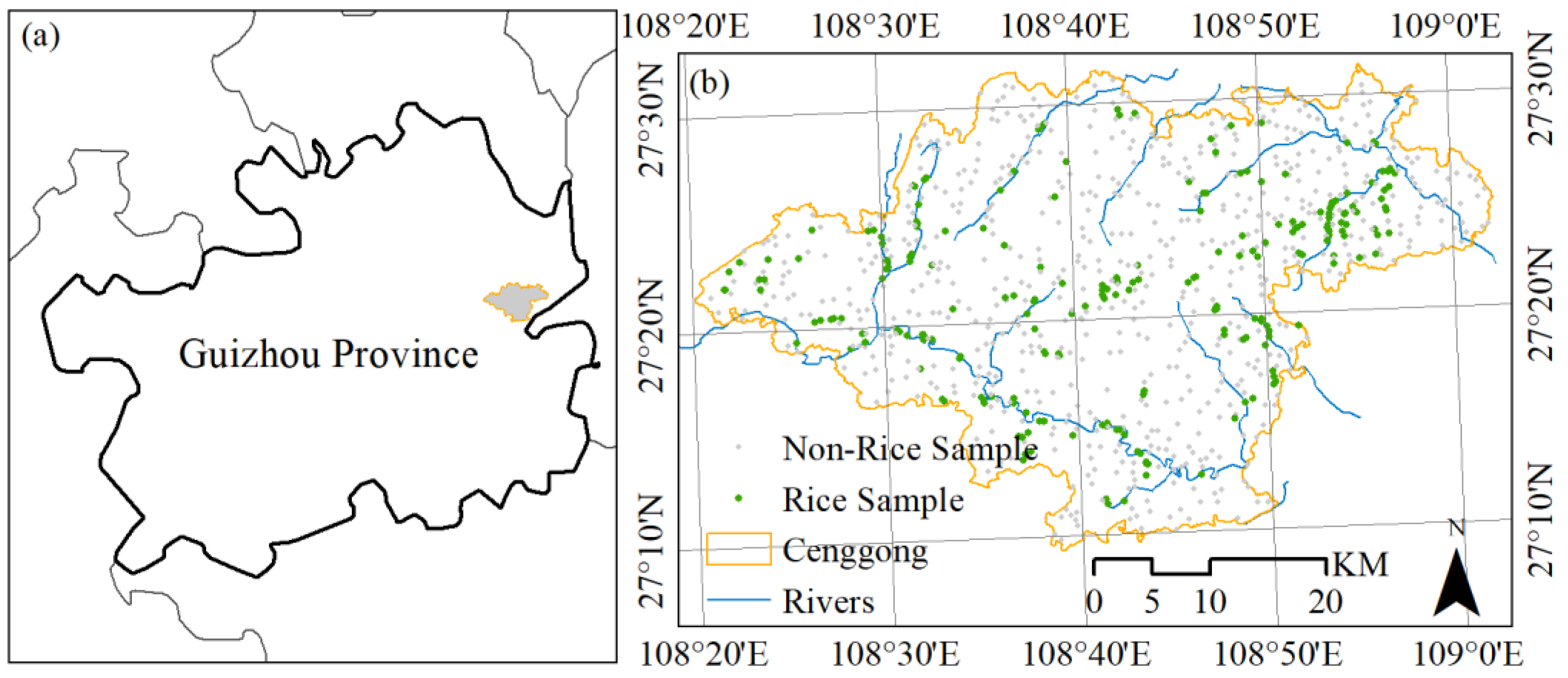
2.1. Study Area

The study area, Cengong County, is located in the eastern part of Guizhou Province, China (longitude 108°20′E to 109°03′E and latitude 27°09′N to 27°32′N) (Figure 1). Cengong has a total area of 1486.5 km², and elevations vary between 330 m and 1359.9 m. The hilly terrain in Cengong typifies a complex landscape. According to a field survey, due to the topography and well-developed roads, paddy rice fields are mainly distributed in the intermountain basins (local name “Bazi”), which are generally fragmented, relatively small, and irregular. The major land cover categories are forest, built-up, water, and cropland, where the cropland includes upland, paddy fields, and abandoned land; because of the topography restriction, the rice fields are usually mixed with other croplands. It has a humid subtropical climate (Köppen Cfa), with distinct seasons and abundant precipitation. The annual average temperature ranges between 15.7 °C and 17.1 °C, and the annual precipitation ranges between 1005.6 mm and 1403.5 mm, which is mainly concentrated in May and June. Cengong County is the only national hybrid rice seed production base in Guizhou Province, and single-cropped rice is the predominant cultivar. The growing season for paddy rice is from May to September.

2.2. Datasets

2.2.1. Time Series Landsat Data

All available Landsat TM, ETM+, and OLI Collection 2 Level 2 products from 2000 to 2020 for Worldwide Reference System-2 (WRS-2) 126/041 with more than 20% clear observations were downloaded from the USGS EROS Science Processing Architecture on Demand Interface (https://espa.cr.usgs.gov/ (accessed on 26 February 2022)), including surface reflectance, brightness temperature (BT), and quality assurance (QA) bands. The QA band can provide the mask of clouds and cloud shadows generated by the CFmask (C version of Fmask) algorithm [46]. The images for Landsat TM, Landsat ETM+, and Landsat OLI were 93, 156, and 63, respectively (Figure 2).

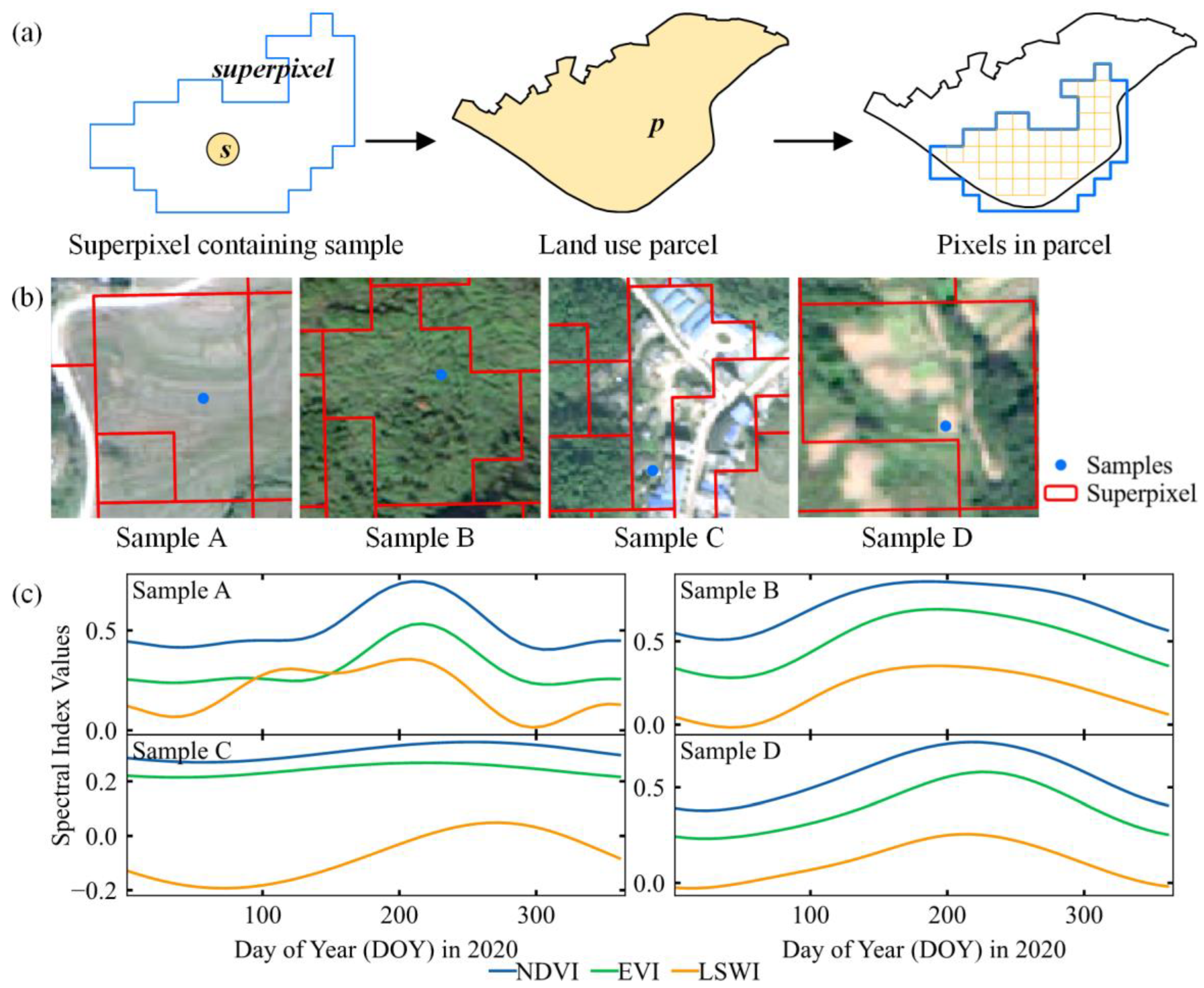
2.2.2. Sample Points

Pure pixels were generated as sample points from the land use map in 2019, the field survey in July 2019, and Tianditu online images [47]. This land use map was provided by the Bureau of Natural Resources of Cengong. The land use map was reclassified to paddy fields, other crops, forests, shrubs, wetlands, built-up, water, and barren. A total of 2500 random sample points were generated in the parcels containing at least six connected Landsat pixels using the Create Random Points tool in ArcGIS Pro 2.8.1 software from ESRI (Redlands, CA, USA). The ground survey was conducted in July 2019 in Cengong County. During the field survey, a handheld data collector (Trimble GeoExplorer 6000, Trimble, Inc. Sunnyvale, CA, USA), which records location with high accuracy, was used to obtain the latitude and longitude of rice-dominated surrounding plots, and a total of 43 points were recorded. The field survey sample points and randomly generated points were merged and further interpreted carefully by using the corresponding Tianditu high-resolution images to exclude the points for which a confident interpretation could not be made.

2.2.3. Agriculture Statistical Data

Agricultural statistics for Cengong were provided by the Bureau of Agriculture and Rural Affairs of Cengong. Statistical data contain estimations of the paddy-rice-sown area from 2004 to 2017. The statistical data for the paddy-rice-sown areas were used to verify the agreement between the government statistics data and our results.

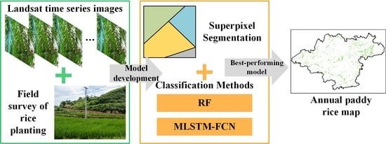
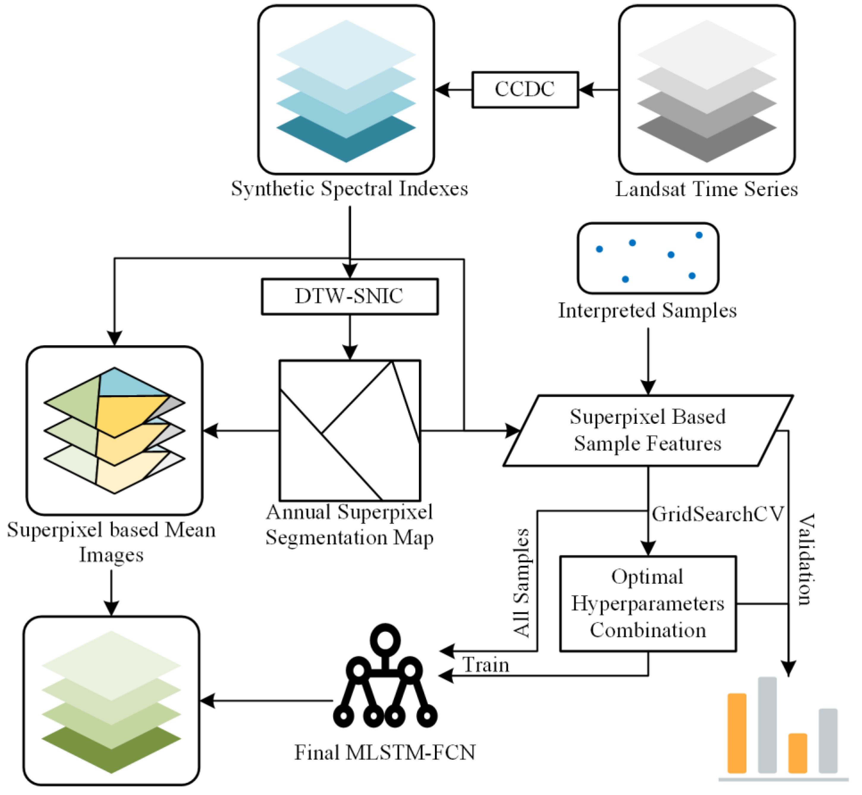
2.3. Proposed Superpixel-Based MLSTM-FCN for Mapping Paddy Rice

Figure 3 shows the flowchart of the superpixel-based MLSTM-FCN for mapping paddy rice. First, the Continuous Change Detection and Classification (CCDC) algorithm was used to synthesize cloud-free Landsat time series, and then SIs time series were created for each year (Section 2.3.1). Next, a superpixel segmentation method was employed to generate annual superpixel maps (Section 2.3.2), and the superpixel-based training/validation dataset was extracted from superpixel maps and SIs time series (Section 2.3.3). Finally, the MLSTM-FCN was used to identify the paddy rice superpixels from the training data generated in the previous section (Section 2.3.4).

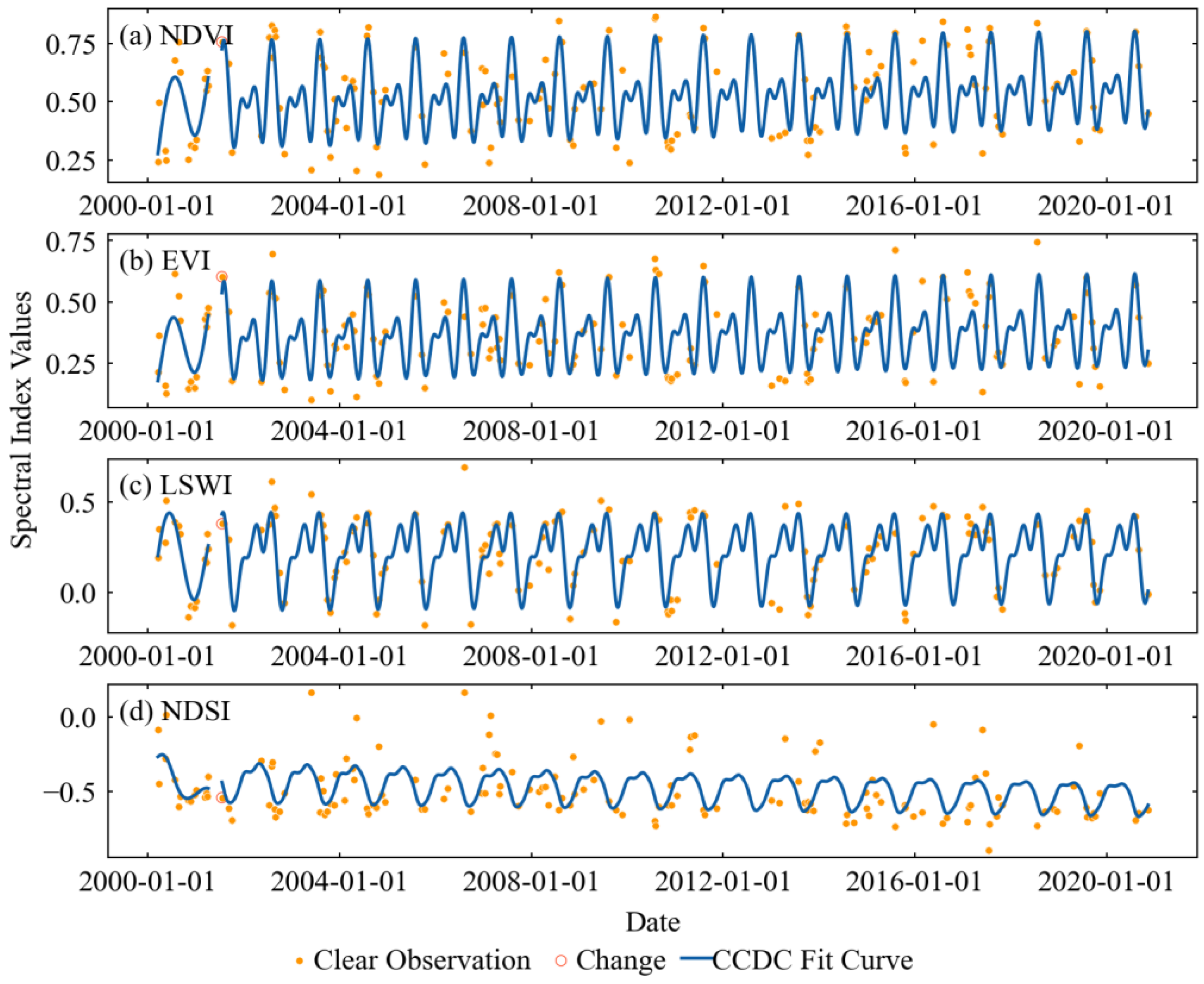
2.3.1. Creating Landsat Spectral Indices Time Series

The CCDC algorithm was employed to generate synthetic Landsat surface reflectance images. The CCDC algorithm is based on the Landsat time series images without (or at least with few) noises such as clouds and cloud shadows, and requires the surface reflectance of Blue, Green, Red, Near-Infrared (NIR), Shortwave Infrared 1 (SWIR1), SWIR2, and the BT of the thermal infrared band as the inputs [48,49]. The clouds and cloud shadows can be screened out by the QA band of Landsat images [46]. For each individual pixel, the CCDC algorithm estimates three sets of Fourier models (e.g., simple (k = 1), advanced (k = 2), and full (k = 3)) according to clear-sky observations, as in Equation (1), and uses the models to detect land cover changes once new Landsat images are collected [50]. If a change is detected, a new time series model will be generated. The CCDC algorithm can also predict Landsat surface reflectance for any desired date based on estimated time series models. The surface reflectance image is synthesized every 8 days to meet the needs of temporal resolution of Landsat images for capturing the paddy rice growth profiles using the CCDC time series models [18,51], which results in 46 synthetic Landsat surface reflectance images per year [48].

$${\widehat{\rho }}_{i,t}=a_{0,i}+c_{1,i}t+{\displaystyle \sum _{k=1}^3(a_{k,i}\cos \frac{2k\pi t}{T}+b_{k,i}\sin \frac{2k\pi t}{T})}$$

(1)

where i is the i-th Landsat band; ${\widehat{\rho }}_{i,t}$ is the predicted surface reflectance for the i-th Landsat band on the Julian date t. $a_{0,i}$, and $c_{1,i}$ are the overall (intercept) and interal-annual change (slope) coefficients for the ith Landsat band; $a_{k,i}$ and $b_{k,i}$ are the intra-annual change coefficients for the i-th Landsat band; k is the temporal frequency of the Fourier component (k = 1, 2, and 3), which is determined by the number of clear-sky observations; and T is the number of days per year (365.25).

Many previous studies have demonstrated that SIs (e.g., NDVI, EVI, LSWI, and NDSI) are useful for paddy rice mapping [25,26,29,30,35,36]. Prior to their input into rice paddy classifiers, the NDVI, EVI, LSWI, and NDSI are computed as follows (Figure 4):

$$\mathrm{NDVI}=\frac{{\rho }_{NIR}-{\rho }_{Red}}{{\rho }_{NIR}+{\rho }_{Red}}$$

(2)

$$\mathrm{EVI}=2.5\times \frac{{\rho }_{NIR}-{\rho }_{Red}}{{\rho }_{NIR}+6{\rho }_{Red}-7.5{\rho }_{Blue}+1}$$

(3)

$$LSWI=\frac{{\rho }_{NIR}-{\rho }_{SWIR}}{{\rho }_{NIR}+{\rho }_{SWIR}}$$

(4)

$$NDSI=\frac{{\rho }_{Green}-{\rho }_{SWIR}}{{\rho }_{Green}+{\rho }_{SWIR}}$$

(5)

where ρ_Blue, ρ_Green, ρ_Red, ρ_NIR, and ρ_SWIR are the surface reflectance from the Blue, Green, Red, NIR, and SWIR1 bands of the synthesized Landsat image, respectively.

2.3.2. Time Series Superpixel Segmentation

Superpixel is a perceptually meaningful cluster of connected similar pixels on images. It captures image redundancy and greatly reduces the complexity of subsequent image processing tasks [52]. In this study, the superpixel was introduced to reduce the salt-and-pepper effect in rice paddy maps [12]. Many approaches have been proposed to generate superpixels, such as Superpixels Extracted via Energy-Driven Sampling (SEEDS) [53], Simple Non-Iterative Clustering (SNIC) [54], and Superpixel Sampling Networks (SSNs) [55]. Among these algorithms, SNIC is faster and requires less computation memory, and is easy to implement at higher dimensions. So, it was modified to generate superpixel maps using the SIs time series.

The original SNIC was designed for RGB images. Several modifications were adopted to apply the SNIC algorithm to time series images. Firstly, since the CIELAB color space is not suitable for time series images, SIs time series were directly input into the SNIC, and a penalty-coefficient-based dynamic time warping (DTW) [56] algorithm was introduced to measure the distance from candidate time series ($t_i$) to the superpixel centroid ($t_k$), as given by Equation (6). Secondly, an adaptive centroid placement method [57] was employed to produce initial centroids according to the information distribution of the images.

$$d_{j,k}=\sqrt{\frac{{\Vert x_i-x_k\Vert }_2^2}{s}+\frac{{\Vert \gamma \_DTW(t_i-t_k)\Vert }_2^2}{m}}$$

(6)

where $x_i$ and $x_k$ are the spatial position of time series $t_i$ and $t_k$, respectively. s and m are the normalizing factors for spatial and time series distances. $\gamma \_DTW$ is the penalty-coefficient-based DTW, which can be written as $\gamma \_DTW=\gamma \times DTW$; the penalty coefficient $\gamma$ is defined as Equation (7).

$$\gamma =1-\frac{l^2}{n_i\times n_k}$$

(7)

where $n_i$ and $n_k$ are the length of time series $t_i$ and $t_k$, respectively; and l is the longest common subsequence (LCS) between $t_i$ and $t_k$.

In this study, considering the size of the paddy rice field in Cengong, the initial superpixel size was set to 5 × 5 (i.e., approximately 150 × 150 m). The connectivity and compactness were set to 4 and 1, respectively. For each year, 46 SIs images were used to produce annual superpixel segmentation maps, and no postprocessing was applied to eliminate small superpixels (see Figure 5b).

2.3.3. Superpixel-Wise Time Series and Sample Data Construction

Pixels within a given superpixel present similar characteristics, which can be represented by the mean feature [58]. In this study, a mean operation was first applied to the pixels within the superpixel, and the mean feature value was assigned to the superpixel as a feature. Finally, four SI (NDVI, EVI, LSWI, and NDSI) time series were constructed for each superpixel.

To ensure the accuracy of samples, the sample points were screened out when land cover changes occurred based on the results of the CCDC algorithm. A total of 235 rice points and 658 non-rice points were collected, and the SIs time series at each sample point were extracted as features of the pixel-wise sample. Additionally, to obtain the superpixel-wise sample features, as is shown in Figure 5a, a superpixel-containing sample s was first overlaid onto the land use map parcel p. Then, the features of the superpixel sample were produced by averaging the SI pixels completely within the superpixel and the parcel p (Figure 5c).

2.3.4. MLSTM-FCN Model for Multivariate Time Series Classification

The MLSTM-FCN was proposed by Karim et al. in 2019 [45]. The MLSTM-FNC augments the full convolution neural network (FCN) module with a long short-term memory (LSTM) module and squeeze-and-excitation blocks [59] to improve the performance. The MLSTM-FCN considers the complex structure of MTS and classifies MTS without heavy preprocessing or feature engineering. Based on the MLSTM-FCN, paddy rice can be classified more accurately and quickly with the consideration of interdependences among different SIs.

In the MLSTM-FCN, feature extractors of the FC block were three temporal convolutional (TC) blocks. Each TC block was followed by a batch normalization (BN) layer with a momentum of 0.99 and an epsilon of 0.001 [60], which was activated by the Rectified Linear Units (ReLUs) [61]. Moreover, the first two TC blocks were succeeded by a squeeze-and-excite block with a reduction ratio r of 16, which was used to recalibrate the input feature maps adaptively [59]. Finally, a global average pooling layer was applied after the final TC block.

Besides the FC block, the MTS was passed through a dimension shuffle layer and conveyed into the LSTM block. The LSTM block contained an LSTM layer followed by a dropout layer, with a dropout rate of 80% to mitigate overfitting. Finally, the results obtained from the FC block and the LSTM block were merged and input into a SoftMax classification layer to produce the final classification result.

2.4. Experiment Design

2.4.1. Methods for Comparison

The pixel-based MLSTM-FCN and RF classifier were used for comparison. RF is an ensemble learning algorithm for classification based on the bagging technique, which is suitable for processing high-dimensional data and prevents overfitting [62].

2.4.2. Model Training and Mapping

The pixel-based (pixel MLSTM-FCN) classifier and superpixel-based classifiers (superpixel MLSTM-FCN and superpixel RF) were trained with pixel-wise and superpixel-wise samples, respectively. The 46 SIs (including the NDVI, EVI, LSWI, and NDSI every 8 days) time series images produced in a year were entered into the MLSTM-FCN classifier and the RF classifier. For the RF classifier, the SI values of each period of the time series were taken as independent features, and important features were selected using SelectFromModel in sklearn according to the importance of the feature.

For tuning the hyperparameters of the MLSTM-FCN and RF, a grid search with cross-validation (GridSearchCV) was employed. According to the specified parameter values, the GridSearchCV generated the best candidates by establishing models with each hyperparameter combination and using 10-fold cross-validation to evaluate each model. The hyperparameter combination with the highest OA was obtained.

Table 1. The search hyperparameters combinations of MLSTM-FCN and RF.

Model	Hyperparameter	Candidate Values
MLSTM-FCN	LSTM hidden size	4, 8, 16, 64, 128
	TC kernel size 1	3, 5, 8
	TC filters 2	8, 16, 32, 64, 128
	epoch	150, 200
RF	n_estimators	[1, 10, 100] 3
	max_depth	[5, 1, 15]

¹ Kernel size of three TC blocks was set to [TC kernel size, 5, 3]. ² Filters of three TC blocks were [filters, 2× filters, filters]. ³ A series number from 1 to 100, at intervals of 10.

shows the hyperparameter combinations used to search for optimal hyperparameter combinations of the classifiers. Then, a final model was trained with all sample data and optimal hyperparameter combination after searching. The other hyperparameters, including learning rate, dropout value, and loss function for the MLSTM-FCN, max_features, min_samples_leaf, and min_samples_split for RF, were set as the default values.

2.4.3. Performance Evaluation

To assess the performance of the paddy rice classifier, 10-fold cross-validation was conducted to evaluate the model established with the optimal hyperparameter combination; the average OA, Producer’s Accuracy (PA), User’s Accuracy (UA), and kappa coefficient of 10 times validation were analyzed. Considering the TP as correctly classified paddy rice samples, TN as the number of accurately identified non-paddy rice samples, FN as paddy rice classified as non-paddy rice, and FP as wrongly classified paddy rice, the performance metrics of classifiers can be defined as Equations (8)–(12).

$$OA=\frac{TP+TN}{TN+TP+FN+FP}$$

(8)

$$PA=\frac{TP}{TP+FN}$$

(9)

$$UA=\frac{TP}{TP+FP}$$

(10)

$$kappa=\frac{OA-p_e}{1-p_e}$$

(11)

$$p_e=\frac{(TP+FN)\times (TP+FP)+(TN+FP)\times (TN+FN)}{{(TP+TN+FP+FN)}^2}$$

(12)

In this study, the CCDC algorithm used to generate synthetic Landsat surface reflectance images was the Matlab procedure (https://github.com/GERSL/CCDC, (accessed on 20 November 2021)). Other data processes were carried out with Python, and the paddy rice classifiers were developed and evaluated using the scikit-learn and PyTorch packages established in Python. The classifiers were trained and executed on a workstation with 2 Intel Xeon E5-2650 processors, NVIDIA GeForce RTX 1080Ti (12 GB), and a memory of 128 GB.

3. Results

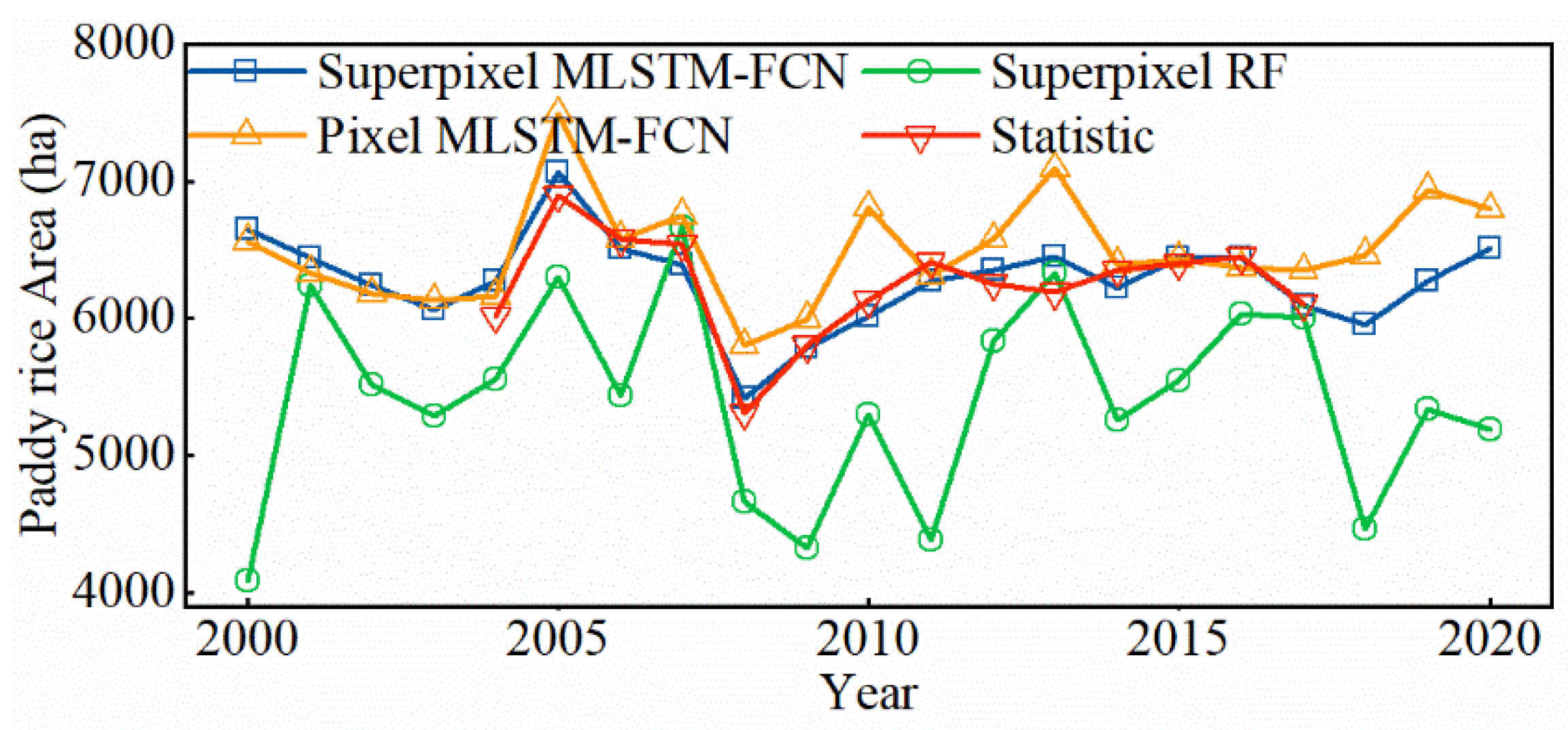
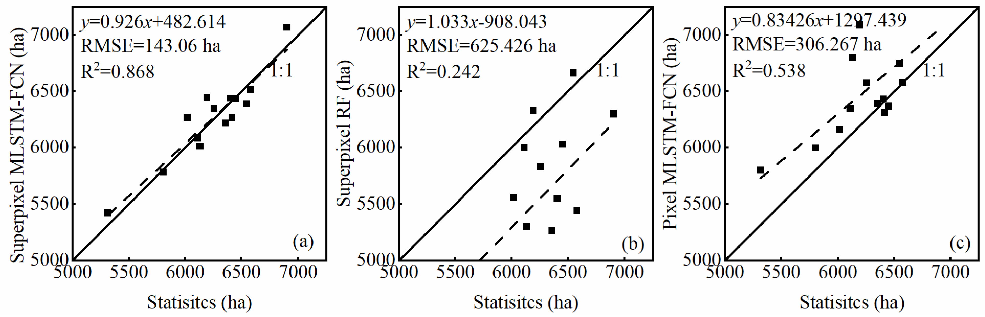
3.1. Performance Evaluation and Comparison with Agriculture Statistical Data

With the validation samples given in Section 2.2.3 and Figure 1, the performance of annual paddy rice classifiers was evaluated, as listed in

Table 2. Overall Accuracy (OA), Producer’s Accuracy (PA), User’s Accuracy (UA), and kappa of the annal paddy rice classifiers. Bold font and underlined values represent the maximum values of evaluation metrics for comparing superpixel MLSTM-FCN with superpixel RF and pixel MLSTM-FCN, respectively.

Year	Pixel MLSTM-FCN				Superpixel MLSTM-FCN				Superpixel RF
	OA	PA	UA	kappa	OA	PA	UA	kappa	OA	PA	UA	kappa
2000	0.9577	0.9259	0.9288	0.8738	0.9640	0.9615	0.9170	0.9124	0.9612	0.9208	0.9436	0.9042
2001	0.9562	0.9219	0.9371	0.8807	0.9552	0.9411	0.9187	0.8950	0.9587	0.9393	0.9222	0.9004
2002	0.9453	0.9130	0.9032	0.8556	0.9547	0.9329	0.9111	0.8887	0.9563	0.9435	0.9125	0.8946
2003	0.9691	0.9549	0.9478	0.8861	0.9712	0.9549	0.9544	0.9333	0.9642	0.9438	0.9356	0.9131
2004	0.9698	0.9656	0.9332	0.8890	0.9674	0.9615	0.9258	0.9201	0.9581	0.9304	0.9275	0.8981
2005	0.9716	0.9551	0.9463	0.9132	0.9701	0.9572	0.9381	0.9254	0.9685	0.9652	0.9321	0.9247
2006	0.9626	0.9484	0.9294	0.9012	0.9668	0.9564	0.9290	0.9180	0.9564	0.9304	0.9249	0.8943
2007	0.9662	0.9716	0.9164	0.8952	0.9617	0.9681	0.9133	0.9109	0.9618	0.9435	0.9261	0.9068
2008	0.9735	0.9624	0.9490	0.9359	0.9710	0.9611	0.9406	0.9294	0.9735	0.9522	0.9589	0.9356
2009	0.9549	0.9327	0.9157	0.8677	0.9609	0.9416	0.9264	0.9049	0.9566	0.9213	0.9286	0.8937
2010	0.9764	0.9600	0.9593	0.9139	0.9701	0.9620	0.9397	0.9285	0.9598	0.9346	0.9274	0.9022
2011	0.9642	0.9449	0.9357	0.9026	0.9721	0.9584	0.9491	0.9332	0.9603	0.9263	0.9369	0.9024
2012	0.9665	0.9656	0.9218	0.9072	0.9680	0.9656	0.9244	0.9214	0.9661	0.9522	0.9345	0.9180
2013	0.9681	0.9476	0.9468	0.9138	0.9667	0.9449	0.9463	0.9210	0.9600	0.9261	0.9371	0.9018
2014	0.9527	0.9238	0.9134	0.8787	0.9582	0.9323	0.9249	0.8977	0.9561	0.9350	0.9203	0.8944
2015	0.9682	0.9403	0.9496	0.9125	0.9655	0.9322	0.9504	0.9149	0.9626	0.9350	0.9368	0.9089
2016	0.9557	0.9360	0.9149	0.8907	0.9626	0.9572	0.9185	0.9101	0.9663	0.9435	0.9408	0.9178
2017	0.9656	0.9355	0.9452	0.8999	0.9577	0.9065	0.9404	0.8917	0.9587	0.9261	0.9318	0.8992
2018	0.9637	0.9394	0.9461	0.9005	0.9638	0.9387	0.9394	0.9117	0.9610	0.9306	0.9403	0.9060
2019	0.9650	0.9393	0.9432	0.9056	0.9636	0.9398	0.9384	0.9123	0.9572	0.9291	0.9254	0.8954
2020	0.9620	0.9234	0.9417	0.8938	0.9652	0.9304	0.9471	0.9129	0.9595	0.9261	0.9360	0.9018
Mean	0.9636	0.9432	0.9345	0.8961	0.9646	0.9478	0.9330	0.9140	0.9611	0.9360	0.9323	0.9054

. The results indicate that the OA, PA, UA, and kappa of the annual paddy rice classifiers differed across the study period. For the superpixel MLSTM-FCN, the OA, PA, UA, and kappa values were 0.9547–0.9721, 0.9065–0.9681, 0.9111–0.9544, and 0.8887–0.9333, respectively. The metric values suggested that most samples in the validation dataset were classified correctly with good consistency. The OA, PA, UA, and kappa were 0.9561–0.9735, 0.9208–0.9652, 0.9125–0.589, and 0.8937–0.9356, respectively, for superpixel RF, and 0.9453–0.9764, 0.9130–0.9716, 0.903–0.9593, and 0.8556–0.9359 for pixel MLSTM-FCN, respectively. Compared with superpixel RF, the OA, PA, and kappa of the superpixel MLSTM-FCN were 0.17–1.23%, 0.19–4.141%, and 0.08–3.41% higher in most of the years since 2000 (at least 15 years). In contrast, UA was 0.44–2.01% higher in approximately half of the years and 0.10–2.37% lower in other years (the higher metrics values are shown in Table 2 in bold font). The OA and UA of the pixel MLSMT-FCN were higher than those of the superpixel MLSMT-FCN in approximately half of the years (around 1–2 years), which suggests that the MLSTM-FCN achieved a very close performance on different datasets. The kappa and PA of the pixel MLSTM-FCN were 0.26–5.33% and 0.05–3.84% lower than those of the superpixel MLSTM-FCN in 19 years (except 2008 and 2017) and 15 years, respectively (the higher metrics values are shown in Table 2 as underlined values). It is noteworthy that all the classifiers used in this study appeared to be reasonably accurate. On average, the superpixel MLSMT-FCN produced slightly higher values of OA (0.9646), PA (0.9478), and kappa (0.9140) than the pixel MLSTM-FCN and superpixel RF and had the lowest value of UA (0.9330).

Moreover, the areas of paddy rice mapped by the superpixel MLSTM-FCN, superpixel RF, and pixel MLSTM-FCN were compared with agricultural statistics on rice-sown areas from 2004 to 2017. Figure 6 shows that the temporal profile of paddy rice areas generated by the superpixel MLSTM-FCN was more consistent with the rice-sown area than the paddy rice areas mapped by the pixel MLSTM-FCN and superpixel RF. During 2004–2017, the relative error in areas between annual paddy rice classification maps and agriculture statistics was 0.20–4.15%, 1.74–31.59%, and 0.07–14.55% for the superpixel MLSMT-FCN, superpixel RF, and pixel MLSTM-FCN, respectively. It is worth noting that the superpixel RF mapped paddy rice areas were underestimated in most years, whereas the pixel-MLSTM-FCN-mapped paddy rice areas were overestimated. The comparison of mapped paddy rice areas by three classifiers and statistical rice-sown areas is depicted in Figure 7. The coefficient of determination ($R^2$) in areas between model-mapped paddy rice and statistics was 0.868, 0.538, and 0.242 for the superpixel MLSTM-FCN, pixel MLSTM-FCN, and pixel MLSTM-FCN, respectively. The root mean square error (RMSE) was 143.060 ha, 306.267 ha, and 625.426 ha for the superpixel MLSTM-FCN, pixel MLSTM-FCN, and pixel MLSTM-FCN, respectively.

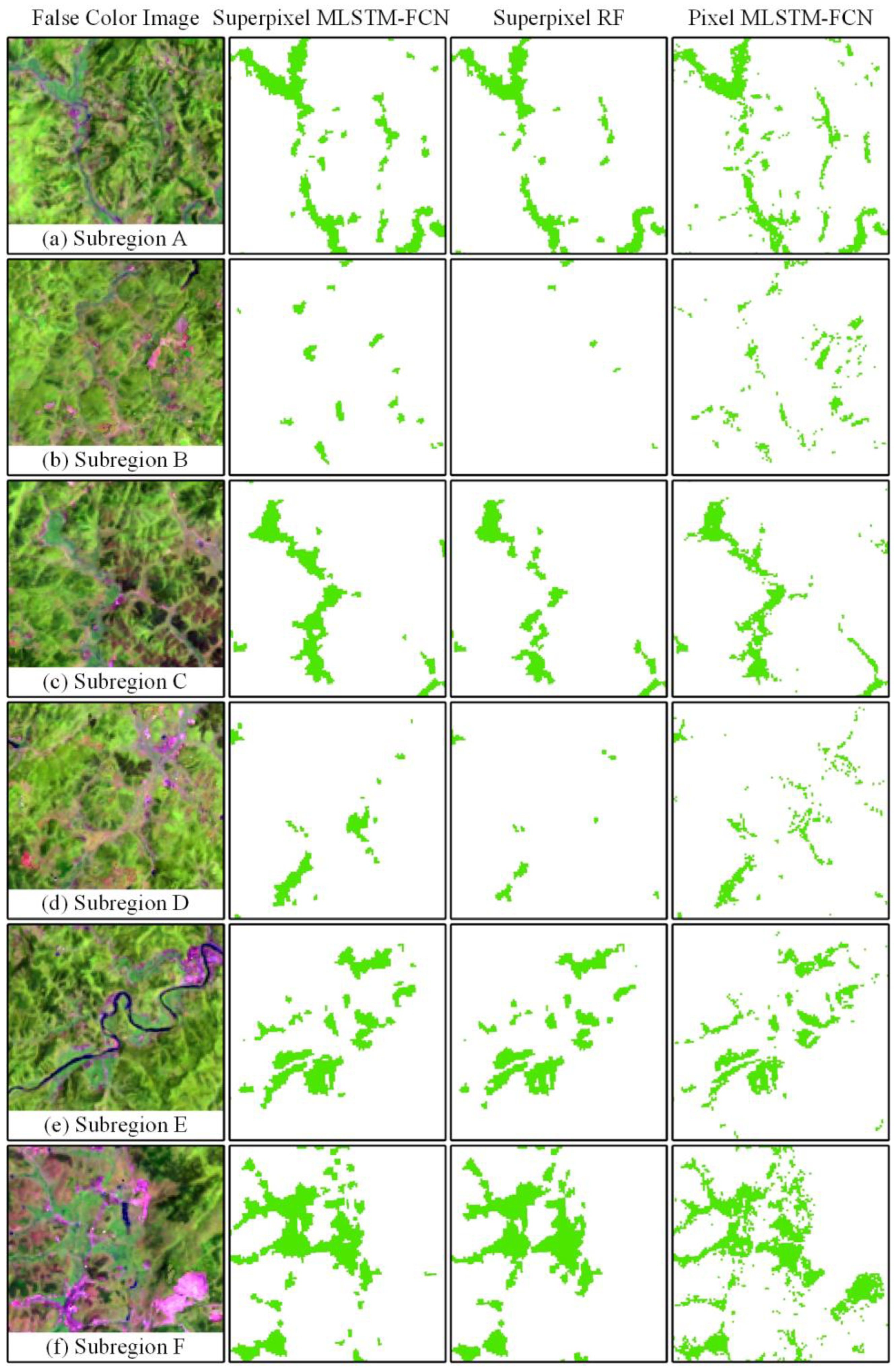
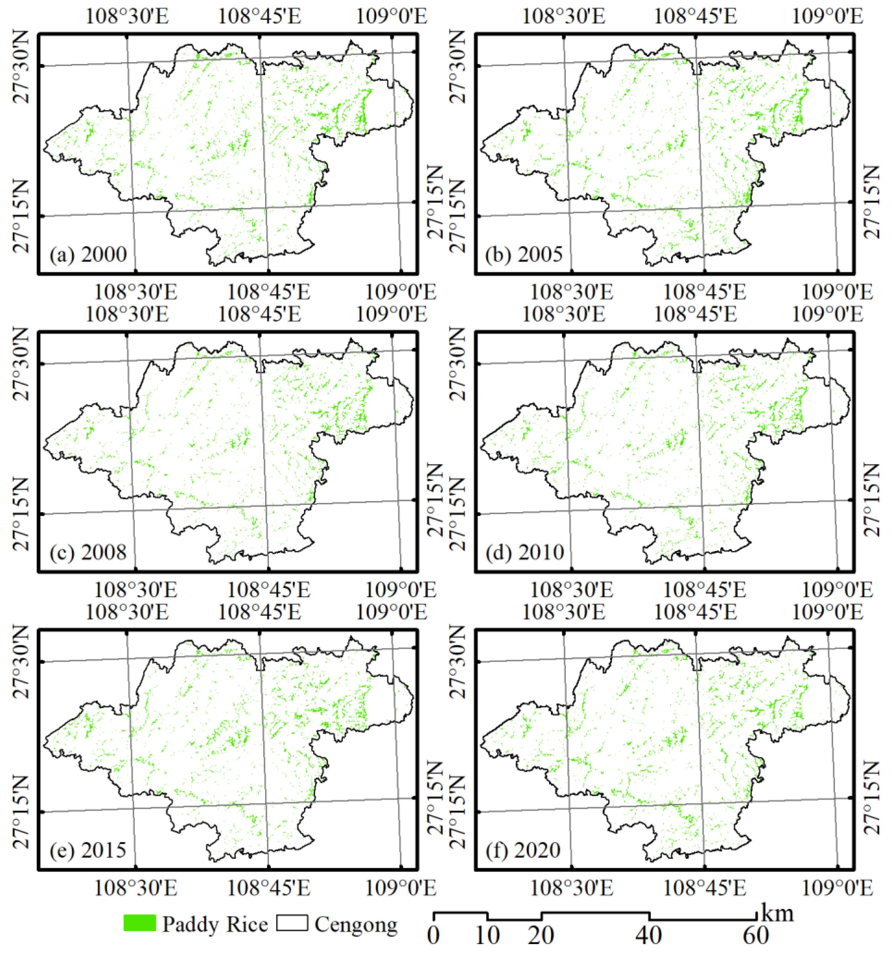
3.2. Visual Assessment of Paddy Rice Mapping Results

The classification maps of the superpixel MLSMT-FCN, superpixel RF, and pixel MLSTM-FCN are shown in Figure 8 to describe the spatial distribution of paddy rice in 2020. The local paddy rice classification results and the false-color image of some representative sites (subregions A–F in Figure 8a) are presented in Figure 9. The classified rice paddies were usually small and scattered. The classified rice paddies of models were mainly distributed in the intermountain basins (locally named “Bazi”) along the rivers, which is shown in the river map in Figure 1b.

Figure 9a–f confirm that the superpixel MLSMT-FCN achieved much higher classification accuracy than the other two methods. The pixel MLSMT-FCN generally identifies more rice paddies, and the superpixel RF classifier identified fewer rice paddies. Rice paddies with larger areas could be identified correctly by all the classifiers that were used in this study (Figure 9a,c,e). The major difference among paddy rice maps generated by three classifiers was the classification of edge pixels (mixed with other land cover types, such as well-developed roads) (Figure 9d) and smaller rice paddy areas (Figure 9b). As shown in Figure 9, the pixel MLSTM-FCN rice map suffered from the salt-and-pepper effect across the region, mainly caused by commission errors. A reduction in commission error was achieved using the superpixel-based classifier as opposed to pixel-based classifiers (Figure 9).

3.3. Interannual Spatial Distribution of Paddy Rice

Since the superpixel MLSMT-FCN yielded more accurate paddy rice maps, annual paddy rice maps from 2000 to 2020 in Cengong were generated with the superpixel MLSMT-FCN (Figure 10). These maps can describe the temporal dynamics of paddy rice distributions. On a temporal scale, the paddy rice area did not exhibit a significant trend but fluctuated during the different years (Figure 10). The sharp fluctuations in paddy rice areas occurred in 2005 and 2008 (Figure 11). From 2000 to 2003, the paddy rice areas in Cengong gradually declined. From 2004 to 2005, the paddy rice areas increased from 6268.95 ha to 7069.95 ha and decreased from 6390.36 ha to 5422.5 ha from 2007 to 2008., The increasing trend in the paddy rice area that had been seen since 2008 fluctuated until 2020, reaching 6514.02 ha. Figure 11 shows that the changed rice paddies were mainly located at boundary pixels of the field or the smaller plots.

4. Discussion

Compared with traditional machine learning algorithms used for mapping paddy rice regions, deep learning time series classifiers can effectively learn salient characteristics and long-term dependencies of time series to provide better performances without onerous preprocessing or feature engineering [63,64]. The superpixel MLSTM-FCN could map annual paddy rice accurately with available Landsat images in complex landscape regions, and its accuracy assessment indicated a better performance than that of superpixel RF. The superpixel RF usually omitted the edge pixels and rice paddies within small areas (Figure 9), which may have been caused by the input features of RF. The input features of RF were the SI values of each period in the time series, which were taken as independent features. Therefore, the RF classifier could capture the temporal correlation of SIs time series. These characteristics are usually used to represent the phenology of paddy rice and have been proven to play a critical role in mapping paddy rice in previous studies [6,14,26]. Consequently, when using traditional machine learning algorithms to map paddy rice, robust feature engineering is required to extract the temporal characteristics as part of the inputs. In addition, the spatial context plays a major role and provides inherent information about the target pixels in remote sensing image classification [30]. The DTW-SINC algorithm was employed to produce superpixel segmentation maps, and mean features were obtained based on superpixel segmentation to describe the spatial feature information of each superpixel. The well-trained MLSMT-FCN with superpixel features was more robust in resisting the salt-and-pepper noise and fragmentation than the pixel MLSTM-FCN, as clearly shown in Figure 9. Therefore, integrating more robust spectral, spatial, and temporal feature extraction into a single model for improving classification accuracy would be worth in-depth research.

Although the superpixel MLSMT-FCN in this study presented satisfactory paddy rice maps, the superpixel LSTM-FCN also exhibited misclassification in paddy rice maps. The synthetic SIs time series images relied on the change detection results from the CCDC algorithm. That algorithm has commission and omission errors in land change detection, especially for land cover types that have higher intra-annual variation, such as agriculture [48,49], and these errors will undermine the time series models used to generate synthetic surface reflectance images and be inherited in the final paddy rice maps. In addition, the misclassification pixels were usually found at the boundaries of the rice paddies, which was also confirmed by previous studies [16]. This finding suggests that using Landsat images with a spatial resolution of 30 m may be insufficient for classifying boundary pixels for small rice paddies. Additionally, land cover with similar spectral and phenological characteristics is often misclassified as paddy rice fields, which leads to noteworthy commission errors. The misclassified land cover mainly includes aquatic plants, such as lotus, abandoned paddies with weeds, and the shadows cast by buildings or topography [12,34,48]. Thus, methods that can combine neighborhood information [65] and high-spatial-resolution satellite images could potentially reduce the misclassification and provide more accurate paddy rice maps in future research.

Based on the spatiotemporal distribution of the annual paddy rice maps in this study, the declining trend from 2000 to 2004 was consistent with the decline in the rice-sown areas in China [66]. The paddy rice areas increased sharply in 2005, and declined severely in 2008, followed by increasing fluctuations until 2020. The possible reasons for the paddy rice area increase in 2005 may be that the government provided a series of special support policies to farmers, such as adopting a reduction in or exemption from agriculture tax and directly subsidizing grain planting while substantially increasing grain purchase prices [67]. In contrast, the increased prices of agricultural inputs (e.g., seeds, fertilizers, and chemicals) reduced farmers’ willingness and confidence to plant crops, resulting in a severe decrease in paddy rice areas in 2008. Since 2008, the Chinese government has implemented a series of policies to promote farmland circulation, which have directly re-inspired the restoration of paddy rice planting.

5. Conclusions

This study proposed a framework that combined superpixel segmentation and deep learning for mapping paddy rice in complex landscape regions with all available Landsat images. Superpixel segmentation and deep learning were combined to extract spectral, spatial, and temporal features of rice paddies. The coupling of deep learning and superpixel segmentation could effectively improve the classification accuracy and reduce the misclassification of the paddy rice map. Compared with county statistics data, the results from using the superpixel MLSTM-FCN were more consistent. The validation results also show that the proposed method had an OA of 0.9547–0.9721, which indicated that the proposed method outperformed pixel-based methods and traditional machine learning algorithms. The dynamics of rice paddies over the last two decades were analyzed, and the policies and the cost of agricultural inputs had greatly affected farmers’ willingness to plant. The resulting maps could provide useful information for policymakers in identifying the dynamics of the paddy rice area, which should be greatly helpful for planning government interventions to promote rice production effectively. The success of this framework verified the necessity of integrating domain knowledge with deep learning techniques for agriculture studies. More research should be conducted to verify the applicability of the proposed method for mapping paddy rice in other complex landscape regions, such as South China. Further, to avoid the irregular availability of remote sensing images, the time series inputs were generated by the CCDC algorithm, which is a heavy computation cost method, and this may limit the applicability of this method in a wider range of regions. Thus, improving the model’s ability to handle the irregular data available without heavy computation is necessary in the future.

References

1. Nie, L.; Peng, S. Rice Production in China. In Rice Production Worldwide; Chauhan, B.S., Jabran, K., Mahajan, G., Eds.; Springer International Publishing: Cham, Germany, 2017; pp. 33–52. ISBN 978-3-319-47514-1. [Google Scholar]
2. Zhang, H.; He, B.; Xing, J.; Lu, M. Spatial and temporal patterns of rice planthopper populations in South and Southwest China. Comput. Electron. Agric. 2022, 194, 106750. [Google Scholar] [CrossRef]
3. Cheng, J. Rice Planthoppers in the Past Half Century in China. In Rice Planthoppers: Ecology, Management, Socio Economics and Policy; Heong, K.L., Cheng, J., Escalada, M.M., Eds.; Zhejiang University Press: Hangzhou, China, 2015; pp. 1–32. ISBN1 978-94-017-9534-0. ISBN2 978-94-017-9535-7. [Google Scholar]
4. Thenkabail, P.S. Remote Sensing of Global Croplands for Food Security; CRC Press: Boca Raton, FL, USA, 2009; ISBN 9781420090109. [Google Scholar]
5. Liu, J.; Kuang, W.; Zhang, Z.; Xu, X.; Qin, Y.; Ning, J.; Zhou, W.; Zhang, S.; Li, R.; Yan, C.; et al. Spatiotemporal characteristics, patterns, and causes of land-use changes in China since the late 1980s. J. Geogr. Sci. 2014, 24, 195–210. [Google Scholar] [CrossRef]
6. Dong, J.; Xiao, X. Evolution of regional to global paddy rice mapping methods: A review. ISPRS J. Photogramm. Remote Sens. 2016, 119, 214–227. [Google Scholar] [CrossRef] [Green Version]
7. Bouman, B.; Humphreys, E.; Tuong, T.P.; Barker, R. Rice and Water. Adv. Agron. 2007, 92, 187–237. [Google Scholar] [CrossRef]
8. Cao, J.; Cai, X.; Tan, J.; Cui, Y.; Xie, H.; Liu, F.; Yang, L.; Luo, Y. Mapping paddy rice using Landsat time series data in the Ganfu Plain irrigation system, Southern China, from 1988−2017. Int. J. Remote Sens. 2021, 42, 1556–1576. [Google Scholar] [CrossRef]
9. Ciais, P.; Bala, G.; Canadell, J.; Chhabra, A.; DeFries, R.; Galloway, J.; Heimann, M.; Jones, C.; le Quéré, C.; Myneni, R.B.; et al. Carbon and Other Biogeochemical Cycles. In Climate Change 2013: The Physical Science Basis. Contribution of Working Group I to the Fifth Assessment Report of IPCC the Intergovernmental Panel on Climate Change; Stocker, T., Plattner, G.-K., Tignor, M., Allen, S., Boschung, J., Nauels, A., Xia, Y., Bex, V., Midgley, P., Eds.; Cambridge University Press: Cambridge, UK, 2014; pp. 465–570. ISBN 9781107057999. [Google Scholar]
10. Chen, C.; van Groenigen, K.J.; Yang, H.; Hungate, B.A.; Yang, B.; Tian, Y.; Chen, J.; Dong, W.; Huang, S.; Deng, A.; et al. Global warming and shifts in cropping systems together reduce China’s rice production. Glob. Food Secur. 2020, 24, 100359. [Google Scholar] [CrossRef]
11. Di Martino, F.; Pedrycz, W.; Sessa, S. Spatiotemporal extended fuzzy C-means clustering algorithm for hotspots detection and prediction. Fuzzy Sets Syst. 2018, 340, 109–126. [Google Scholar] [CrossRef]
12. Xiao, W.; Xu, S.; He, T. Mapping Paddy Rice with Sentinel-1/2 and Phenology-, Object-Based Algorithm—A Implementation in Hangjiahu Plain in China Using GEE Platform. Remote Sens. 2021, 13, 990. [Google Scholar] [CrossRef]
13. Dong, J.; Xiao, X.; Menarguez, M.A.; Zhang, G.; Qin, Y.; Thau, D.; Biradar, C.M.; Moore, B. Mapping paddy rice planting area in northeastern Asia with Landsat 8 images, phenology-based algorithm and Google Earth Engine. Remote Sens. Environ. 2016, 185, 142–154. [Google Scholar] [CrossRef] [PubMed] [Green Version]
14. Xiao, X.; Boles, S.; Frolking, S.; Li, C.; Babu, J.Y.; Salas, W.; Moore, B. Mapping paddy rice agriculture in South and Southeast Asia using multi-temporal MODIS images. Remote Sens. Environ. 2006, 100, 95–113. [Google Scholar] [CrossRef]
15. Nelson, A.; Setiyono, T.; Rala, A.; Quicho, E.; Raviz, J.; Abonete, P.; Maunahan, A.; Garcia, C.; Bhatti, H.; Villano, L.; et al. Towards an Operational SAR-Based Rice Monitoring System in Asia: Examples from 13 Demonstration Sites across Asia in the RIICE Project. Remote Sens. 2014, 6, 10773–10812. [Google Scholar] [CrossRef] [Green Version]
16. Wang, J.; Huang, J.; Zhang, K.; Li, X.; She, B.; Wei, C.; Gao, J.; Song, X. Rice Fields Mapping in Fragmented Area Using Multi-Temporal HJ-1A/B CCD Images. Remote Sens. 2015, 7, 3467–3488. [Google Scholar] [CrossRef] [Green Version]
17. Thorp, K.R.; Drajat, D. Deep machine learning with Sentinel satellite data to map paddy rice production stages across West Java, Indonesia. Remote Sens. Environ. 2021, 265, 112679. [Google Scholar] [CrossRef]
18. Zhu, L.; Liu, X.; Wu, L.; Liu, M.; Lin, Y.; Meng, Y.; Ye, L.; Zhang, Q.; Li, Y. Detection of paddy rice cropping systems in southern China with time series Landsat images and phenology-based algorithms. GIScience Remote Sens. 2021, 58, 733–755. [Google Scholar] [CrossRef]
19. Nguyen, D.B.; Wagner, W. European Rice Cropland Mapping with Sentinel-1 Data: The Mediterranean Region Case Study. Water 2017, 9, 392. [Google Scholar] [CrossRef]
20. Nguyen, D.B.; Gruber, A.; Wagner, W. Mapping rice extent and cropping scheme in the Mekong Delta using Sentinel-1A data. Remote Sens. Lett. 2016, 7, 1209–1218. [Google Scholar] [CrossRef]
21. Bazzi, H.; Baghdadi, N.; El Hajj, M.; Zribi, M.; Minh, D.H.T.; Ndikumana, E.; Courault, D.; Belhouchette, H. Mapping Paddy Rice Using Sentinel-1 SAR Time Series in Camargue, France. Remote Sens. 2019, 11, 887. [Google Scholar] [CrossRef] [Green Version]
22. Torbick, N.; Chowdhury, D.; Salas, W.; Qi, J. Monitoring Rice Agriculture across Myanmar Using Time Series Sentinel-1 Assisted by Landsat-8 and PALSAR-2. Remote Sens. 2017, 9, 119. [Google Scholar] [CrossRef] [Green Version]
23. Yang, S.; Shen, S.; Li, B.; Le Toan, T.; He, W. Rice Mapping and Monitoring Using ENVISAT ASAR Data. IEEE Geosci. Remote Sens. Lett. 2008, 5, 108–112. [Google Scholar] [CrossRef]
24. Boschetti, M.; Busetto, L.; Manfron, G.; Laborte, A.; Asilo, S.; Pazhanivelan, S.; Nelson, A.D. PhenoRice: A method for automatic extraction of spatio-temporal information on rice crops using satellite data time series. Remote Sens. Environ. 2017, 194, 347–365. [Google Scholar] [CrossRef] [Green Version]
25. Xiao, X.; Boles, S.; Liu, J.; Zhuang, D.; Frolking, S.; Li, C.; Salas, W.; Moore, B. Mapping paddy rice agriculture in southern China using multi-temporal MODIS images. Remote Sens. Environ. 2005, 95, 480–492. [Google Scholar] [CrossRef]
26. Dong, J.; Xiao, X.; Kou, W.L.; Qin, Y.; Zhang, G.; Li, L.; Jin, C.; Zhou, Y.; Wang, J.; Biradar, C.M.; et al. Tracking the dynamics of paddy rice planting area in 1986-2010 through time series Landsat images and phenology-based algorithms. Remote Sens. Environ. 2015, 160, 99–113. [Google Scholar] [CrossRef]
27. Zhang, G.; Xiao, X.; Dong, J.; Kou, W.L.; Jin, C.; Qin, Y.; Zhou, Y.; Wang, J.; Menarguez, M.A.; Biradar, C.M. Mapping paddy rice planting areas through time series analysis of MODIS land surface temperature and vegetation index data. ISPRS J. Photogramm. Remote Sens. 2015, 106, 157–171. [Google Scholar] [CrossRef] [PubMed] [Green Version]
28. Shi, J.; Huang, J. Monitoring Spatio-Temporal Distribution of Rice Planting Area in the Yangtze River Delta Region Using MODIS Images. Remote Sens. 2015, 7, 8883–8905. [Google Scholar] [CrossRef] [Green Version]
29. Kontgis, C.; Schneider, A.; Ozdogan, M. Mapping rice paddy extent and intensification in the Vietnamese Mekong River Delta with dense time stacks of Landsat data. Remote Sens. Environ. 2015, 169, 255–269. [Google Scholar] [CrossRef]
30. Zhang, M.; Lin, H.; Wang, G.; Sun, H.; Fu, J. Mapping Paddy Rice Using a Convolutional Neural Network (CNN) with Landsat 8 Datasets in the Dongting Lake Area, China. Remote Sens. 2018, 10, 1840. [Google Scholar] [CrossRef] [Green Version]
31. Qiu, B.; Lu, D.; Tang, Z.; Chen, C.; Zou, F. Automatic and adaptive paddy rice mapping using Landsat images: Case study in Songnen Plain in Northeast China. Sci. Total. Environ. 2017, 598, 581–592. [Google Scholar] [CrossRef] [PubMed]
32. Zhang, G.; Xiao, X.; Biradar, C.M.; Dong, J.; Qin, Y.; Menarguez, M.A.; Zhou, Y.; Zhang, Y.; Jin, C.; Wang, J.; et al. Spatiotemporal patterns of paddy rice croplands in China and India from 2000 to 2015. Sci. Total. Environ. 2017, 579, 82–92. [Google Scholar] [CrossRef]
33. Xiao, X.; Boles, S.; Frolking, S.; Salas, W.; Moore III, B.; Li, C.; He, L.; Zhao, R. Observation of flooding and rice transplanting of paddy rice fields at the site to landscape scales in China using VEGETATION sensor data. Int. J. Remote Sens. 2002, 23, 3009–3022. [Google Scholar] [CrossRef]
34. Nguyen, T.T.H.; Bie, C.A.J.M.D.; Ali, A.; Smaling, E.M.A.; Chu, T.H. Mapping the irrigated rice cropping patterns of the Mekong delta, Vietnam, through hyper-temporal SPOT NDVI image analysis. Int. J. Remote Sens. 2012, 33, 415–434. [Google Scholar] [CrossRef]
35. Zhang, X.; Wu, B.; Ponce-Campos, G.E.; Zhang, M.; Chang, S.; Tian, F. Mapping up-to-date paddy rice extent at 10 M resolution in China through the integration of optical and synthetic aperture radar images. Remote Sens. 2018, 10, 1200. [Google Scholar] [CrossRef] [Green Version]
36. Clauss, K.; Yan, H.; Kuenzer, C. Mapping Paddy Rice in China in 2002, 2005, 2010 and 2014 with MODIS Time Series. Remote Sens. 2016, 8, 434. [Google Scholar] [CrossRef] [Green Version]
37. Park, S.; Im, J.; Park, S.; Yoo, C.; Han, H.; Rhee, J. Classification and Mapping of Paddy Rice by Combining Landsat and SAR Time Series Data. Remote Sens. 2018, 10, 447. [Google Scholar] [CrossRef] [Green Version]
38. Zhao, H.; Chen, Z.; Jiang, H.; Jing, W.; Sun, L.; Feng, M. Evaluation of Three Deep Learning Models for Early Crop Classification Using Sentinel-1A Imagery Time Series—A Case Study in Zhanjiang, China. Remote Sens. 2019, 11, 2673. [Google Scholar] [CrossRef] [Green Version]
39. Ndikumana, E.; Ho Tong Minh, D.; Baghdadi, N.; Courault, D.; Hossard, L. Deep Recurrent Neural Network for Agricultural Classification using multitemporal SAR Sentinel-1 for Camargue, France. Remote Sens. 2018, 10, 1217. [Google Scholar] [CrossRef] [Green Version]
40. Zhou, Y.; Luo, J.; Feng, L.; Yang, Y.; Chen, Y.; Wu, W. Long-short-term-memory-based crop classification using high-resolution optical images and multi-temporal SAR data. GIScience Remote Sens. 2019, 56, 1170–1191. [Google Scholar] [CrossRef]
41. Du, Z.; Yang, J.; Ou, C.; Zhang, T. Smallholder Crop Area Mapped with a Semantic Segmentation Deep Learning Method. Remote Sens. 2019, 11, 888. [Google Scholar] [CrossRef] [Green Version]
42. Zhao, S.; Liu, X.; Ding, C.; Liu, S.; Wu, C.; Wu, L. Mapping Rice Paddies in Complex Landscapes with Convolutional Neural Networks and Phenological Metrics. GIScience Remote Sens. 2020, 57, 37–48. [Google Scholar] [CrossRef]
43. Bargiel, D. A new method for crop classification combining time series of radar images and crop phenology information. Remote Sens. Environ. 2017, 198, 369–383. [Google Scholar] [CrossRef]
44. Chockalingam, J.; Mondal, S. Fractal-Based Pattern Extraction from Time-Series NDVI Data for Feature Identification. IEEE J. Sel. Top. Appl. Earth Obs. Remote Sens. 2017, 10, 5258–5264. [Google Scholar] [CrossRef]
45. Karim, F.; Majumdar, S.; Darabi, H.; Harford, S. Multivariate LSTM-FCNs for time series classification. Neural Netw. 2019, 116, 237–245. [Google Scholar] [CrossRef] [PubMed] [Green Version]
46. Zhu, Z.; Wang, S.; Woodcock, C.E. Improvement and expansion of the Fmask algorithm: Cloud, cloud shadow, and snow detection for Landsats 4–7, 8, and Sentinel 2 images. Remote Sens. Environ. 2015, 159, 269–277. [Google Scholar] [CrossRef]
47. National Geomatics Center of China. National Platform for Common Geospatial Information Services. Available online: https://www.tianditu.gov.cn/ (accessed on 20 October 2021).
48. Zhu, Z.; Woodcock, C.E.; Holden, C.; Yang, Z. Generating synthetic Landsat images based on all available Landsat data: Predicting Landsat surface reflectance at any given time. Remote Sens. Environ. 2015, 162, 67–83. [Google Scholar] [CrossRef]
49. Zhu, Z.; Woodcock, C.E. Continuous change detection and classification of land cover using all available Landsat data. Remote Sens. Environ. 2014, 144, 152–171. [Google Scholar] [CrossRef] [Green Version]
50. Guan, Y.; Zhou, Y.; He, B.; Liu, X.; Zhang, H.; Feng, S. Improving Land Cover Change Detection and Classification with BRDF Correction and Spatial Feature Extraction Using Landsat Time Series: A Case of Urbanization in Tianjin, China. IEEE J. Sel. Top. Appl. Earth Obs. Remote Sens. 2020, 13, 4166–4177. [Google Scholar] [CrossRef]
51. Onojeghuo, A.O.; Blackburn, G.A.; Wang, Q.; Atkinson, P.M.; Kindred, D.; Miao, Y. Rice crop phenology mapping at high spatial and temporal resolution using downscaled MODIS time-series. GIScience Remote Sens. 2018, 55, 659–677. [Google Scholar] [CrossRef] [Green Version]
52. Achanta, R.; Shaji, A.; Smith, K.; Lucchi, A.; Fua, P.; Süsstrunk, S. SLIC superpixels compared to state-of-the-art superpixel methods. IEEE Trans. Pattern Anal. Mach. Intell. 2012, 34, 2274–2282. [Google Scholar] [CrossRef] [Green Version]
53. van den Bergh, M.; Boix, X.; Roig, G.; Capitani, B.D.; van Gool, L. SEEDS: Superpixels Extracted via Energy-Driven Sampling. In Proceedings of the European Conference on Computer Vision, Florence, Italy, 7–13 October 2012; Springer: Berlin, Germany, 2012; pp. 13–26. [Google Scholar]
54. Achanta, R.; Susstrunk, S. Superpixels and Polygons Using Simple Non-iterative Clustering. In Proceedings of the 2017 IEEE Conference on Computer Vision and Pattern Recognition (CVPR), Honolulu, HI, USA, 21–26 July 2017; IEEE: Piscataway, NJ, USA, 2017; pp. 4895–4904, ISBN 978-1-5386-0457-1. [Google Scholar]
55. Jampani, V.; Sun, D.; Liu, M.-Y.; Yang, M.-H.; Kautz, J. Superpixel Sampling Networks. In Computer Vision—ECCV 2018, Proceedings of the Part VII: 15th European Conference, Munich, Germany, 8–14 September 2018; Ferrari, V., Hebert, M., Sminchisescu, C., Weiss, Y., Eds.; Springer: Cham, Switzerland, 2018; pp. 363–380. ISBN 9783030012335. [Google Scholar]
56. Li, H.; Du, T. Multivariate time-series clustering based on component relationship networks. Expert Syst. Appl. 2021, 173, 114649. [Google Scholar] [CrossRef]
57. Bandara Senanayaka, J.; Thilanka Morawaliyadda, D.; Tharuka Senarath, S.; Indika Godaliyadda, R.; Parakrama Ekanayake, M. Adaptive Centroid Placement Based SNIC for Superpixel Segmentation. In Proceedings of the 2020 Moratuwa Engineering Research Conference (MERCon), Moratuwa, Sri Lanka, 28–30 July 2020; IEEE: Piscataway, NJ, USA, 2020; pp. 242–247, ISBN 978-1-7281-9975-7. [Google Scholar]
58. Fang, L.; Li, S.; Duan, W.; Ren, J.; Benediktsson, J.A. Classification of Hyperspectral Images by Exploiting Spectral–Spatial Information of Superpixel via Multiple Kernels. IEEE Trans. Geosci. Remote Sens. 2015, 53, 6663–6674. [Google Scholar] [CrossRef] [Green Version]
59. Hu, J.; Shen, L.; Sun, G. Squeeze-and-Excitation Networks. In Proceedings of the 2018 IEEE/CVF Conference on Computer Vision and Pattern Recognition, Salt Lake City, UT, USA, 18–23 June 2018; IEEE: Piscataway, NJ, USA, 2018. [Google Scholar]
60. Ioffe, S.; Szegedy, C. Batch Normalization: Accelerating Deep Network Training by Reducing Internal Covariate Shift. In Proceedings of the International Conference on Machine Learning, Lille, France, 6–11 July 2015; pp. 448–456. [Google Scholar]
61. Trottier, L.; Giguere, P.; Chaib-draa, B. Parametric Exponential Linear Unit for Deep Convolutional Neural Networks. In Proceedings of the 2017 16th IEEE International Conference on Machine Learning and Applications (ICMLA), Cancun, Mexico, 18–21 December 2017; IEEE: Piscataway, NJ, USA, 2017. [Google Scholar]
62. Breiman, L. Random Forests. Mach. Learn. 2001, 45, 5–32. [Google Scholar] [CrossRef] [Green Version]
63. Karim, F.; Majumdar, S.; Darabi, H.; Chen, S. LSTM Fully Convolutional Networks for Time Series Classification. IEEE Access 2018, 6, 1662–1669. [Google Scholar] [CrossRef]
64. Greff, K.; Srivastava, R.K.; Koutnik, J.; Steunebrink, B.R.; Schmidhuber, J. LSTM: A Search Space Odyssey. IEEE Trans. Neural Netw. Learn. Syst. 2017, 28, 2222–2232. [Google Scholar] [CrossRef] [PubMed] [Green Version]
65. Tan, S.; Chen, L.; Pan, Z.; Xing, J.; Li, Z.; Yuan, Z. Geospatial Contextual Attention Mechanism for Automatic and Fast Airport Detection in SAR Imagery. IEEE Access 2020, 8, 173627–173640. [Google Scholar] [CrossRef]
66. National Bureau of Statistics of China. National Data. Available online: https://data.stats.gov.cn/english/easyquery.htm?cn=E0103 (accessed on 21 December 2020).
67. Xin, L.; Liu, X. Changes of multiple cropping in double cropping rice area of southern China and its policy implications. J. Nat. Resour. 2009, 24, 58–65. [Google Scholar]
Figure 1. Maps of study area and sample points: (a) the yellow scope indicates the study area in Guizhou Province, China; and (b) non-rice and rice represent sample points for training and validating classifiers.
Remotesensing 14 03721 g001
Figure 2. Annual distribution and clear-sky observations of all available Landsat images from 2000 to 2020 in Cengong County (Path/Row: 126/041).
Remotesensing 14 03721 g002
Figure 3. Flowchart of paddy rice mapping in this study. CCDC: Continuous Change Detection and Classification. DTW-SNIC: Dynamic-Time-Warping-based Simple Non-Iterative Clustering. MLSTM-FCN: Multivariate Long Short-Term Memory Full Convolution Neural Network.
Remotesensing 14 03721 g003
Figure 4. Example (longitude: 108.63134233°E, latitude: 27.46887562°N) of CCDC-algorithm-based model fit of (a) NDVI, (b) EVI, (c) LSWI, and (d) NDSI.
Remotesensing 14 03721 g004
Figure 5. Superpixel segmentation map and superpixel-wise time series construction: (a) superpixel-wise sample data construction. (b) The high-resolution true-color image and superpixel segmentation at selected sample points with different land use types. Sample A (rice, longitude: 108.54357776°E, latitude: 27.37971958°N), Sample B (forest, longitude: 108.63321201°E, latitude: 27.27148616°N), Sample C (building, longitude: 108.72232946°E, latitude: 27.37451097°N), and Sample D (other cropland, longitude: 108.92616261°E, latitude: 27.45895508°N). (c) Superpixel-wise temporal profile of NDVI, EVI, and LSWI at four sample points in 2020.
Remotesensing 14 03721 g005
Figure 6. Mapped paddy rice area by three classification models from 2000 to 2020.
Remotesensing 14 03721 g006
Figure 7. Correlations between agricultural statistics and mapped area by (a) superpixel MLSTM-FCN, (b) superpixel RF, and (c) pixel MLSTM-FCN.
Remotesensing 14 03721 g007
Figure 8. Paddy rice mapping results for 2020. (a) Stack of paddy rice maps generated by superpixel MLSTM-FCN (green), superpixel RF (yellow), and pixel MLSTM-FCN (blue). (bd) represent the paddy rice mapping result using (b) superpixel MLSTM-FCN, and (c) pixel MLSTM-FCN, (d) superpixel RF. The red square represents six subregions (subregion A to subregion F) that were used to compare the detailed information created by classifiers.
Remotesensing 14 03721 g008
Figure 9. Local details of paddy rice mapping results of different classifiers in 2020, (af) represent the detailed information at subregion A to subregion F, respectively. False color image was composite by synthetic Landsat surface reflectance image on 28 July 2020 (R: SWIR 1, G: NIR, B: Green).
Remotesensing 14 03721 g009
Figure 10. Paddy rice map generated by superpixel MLSTM-FCN in Cengong during 2000–2020. (a) 2000, (b) 2005, (c) 2008, (d) 2010, (e) 2015, and (f) 2020.
Remotesensing 14 03721 g010
Figure 11. Temporal variation in local detailed paddy rice map at (a) subregion A from 2004 to 2005, (b) subregion A from 2007 to 2008, (c) subregion E from 2004 to 2005, and (d) subregion E from 2007 to 2008.
Remotesensing 14 03721 g011