Abstract
This study implemented a stable Regional Reference Frame in Shanghai, East China (called SHRRF), using seven years of continuous GNSS observations from the Shanghai Continuously Operating Reference System stations (SHCORS) to examine reclaimed coast–land subsidence. A well−distributed core station network suitable for regional applications was derived. The instantaneous station coordinates and seven frame parameters (translations, rotations, and scale) were estimated at each epoch through minimum constraint during the process of aligning SHRRF to the International Terrestrial Reference Frame (ITRF14). The average root mean square error (RMSE) of all stations under SHRRF was within 1.5 mm horizontally and 5 mm vertically for most epochs. Simultaneously, compared with the ITRF14 solutions, the average RMSE for each site at all epochs was reduced by ~30% horizontally and ~10% vertically. A temporal consolidation settlement model of the reclaimed soil under self−weight was established by combining a geotechnical−derived model with high precision permanent GNSS vertical solutions under SHRRF. The model indicates that ~50% of settlements occurred within 3.6 years, with the whole subsidence time being 46 years. SHRRF provides a precise regional reference frame for use in many East China geophysical applications besides reclaimed coast–land settlement including hydrologic loading, microplate motions, and critical structure deformation monitoring.
1. Introduction
With rapid economic development and population growth, the people’s demand for land resources is increasing. The contradiction between limited land resources and people’s needs is becoming more serious, especially in economically developed coastal cities. Shanghai is an important commercial and financial metropolis on the eastern coast of China and has a large population, where land scarcity is also a serious problem. In order to solve the conflict between land supply and demand, the government has continued to backfill land along China’s east coastline since the 1950s [1]. Up to 2008, the accumulated reclaimed area accounted for about 15.8% of the total land area in Shanghai [2]. The government plans to reclaim an additional 1000 km2 of new land in the eastern coastal area (from 121°30′E to 122°10′E; and from 30°45′N to 31°15′N) [3].
Serious land subsidence is the most common geological hazard in the reclaimed area, with the subsidence occasionally exceeding 40% of the entire reclaimed soil layer thickness [2], causing serious property losses and even casualties. Monitoring land subsidence and analyzing the trend of regional surface deformation are the key points to prevent disasters and reduce disaster losses. The Global Navigation Satellite System (GNSS) is a mature technique to monitor the reclaimed land subsidence over the past few decades [4,5,6]. The high precision GNSS technology is a powerful tool for detecting ground displacements and monitoring geological hazards [7,8,9,10].
A well−established reference frame with high accuracy and stability is crucial for monitoring land displacements and structural deformation [11,12]. The International Terrestrial Reference Frame (ITRF) represents the most reliable global reference frame co−rotating with the solid Earth. It is realized through integrating multiple space geodetic techniques to maintain a mm level accuracy by a set of globally distributed core stations [13,14]. However, for regional deformation monitoring and research, the sparse and heterogeneous density of stations makes the ITRF insufficient for detailed study. The regional reference frames with sufficient local coverage provides a complementary service to remedy the geometrical sparsity. Such a regional reference frame is usually aligned to ITRF to maintain high accuracy and stability, and is called the regional realization of ITRF. Presently, many continental−scale and regional−scale geodetic reference frames have been established and aligned to ITRF such as the Stable North America Reference Frame (SNARF and NA12) [15], the European Terrestrial Reference System (ETRS2005 and ETRS2014) [11,16], the Sistema de Referencia Geocéntrico para Las Américas (SIRGAS) [17], the Russian Terrestrial Reference Frame [18], the Stable Puerto Rico and Virgin Islands Reference Frame (SPRVIRF) [19], and the geodetic reference frame in North China (NChina16) [20].
This study aimed to establish a regional reference frame (Regional Reference Frame in Shanghai, East China, hereafter referred to as SHRRF) for the study of reclaimed land subsidence. SHRRF is realized based on observations of the Shanghai Continuously Operating Reference System (SHCORS), which is primarily maintained by the Shanghai Surveying and Mapping Institute. The SHCORS was constructed in 2008, and upgraded in 2011 and 2012. As shown in Figure 1, there are 11 permanent GNSS stations in the SHCORS. Since 2012, station SHJS has been replaced by JSXC, and SSJG has been renamed SJGN.
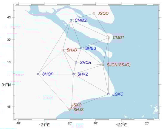
Figure 1.
The station distribution of SHCORS including six core stations (blue squares) and five other stations (red circles). Since 2012, stations SSJG and SHJS have been replaced by SJGN and JSXC, respectively.
2. Methods
The implementation of SHRRF consists of two steps. First, the observations of the regional sub−network and nearby International GNSS Service (IGS) stations were comprehensively analyzed to obtain loosely constrained daily solutions; then, the loose solutions of the regional subnet needed to be merged into the looser solution of the global network. This ad hoc strategy is similar to cluster analysis. Second, the combined loosely constrained daily global solutions were aligned to the ITRF by seven frame parameters (including translations, rotations, and scale) of Helmert transformation through a set of globally distributed core stations. Such an alignment with “minimum constraint” maintains the frame stability while simultaneously preserving the internal solution structure of the regional subnetwork. The details of SHRRF implementation are given in the next sections.
2.1. Data Processing
The 1−HZ observations of the regional sub−network in daily RINEX files from 1 January 2008 to 31 December 2014 corresponding to the GPS weeks from 1460 to 1773 were reprocessed to obtain the daily loosely constrained coordinate solutions by using the GAMIT (V10.6) software package. This sub−network consists of 11 SHCORS and 14 IGS stations in and around China. According to the recommendations by the International Earth Rotation and Reference Systems Service Conventions, the Vienna Mapping Function 1 was used to correct the tropospheric delays and the FES2004 model was used to model the ocean tide loading. The satellite orbits and earth rotation parameters of the IGS final products were adopted in this study [21]. More details of the models and corresponding parameters adopted in the data analysis are listed in Table 1. The regional daily loosely constrained solutions were combined with the loosely constrained global network solutions, which were provided by the University of California, San Diego (ftp://garner.ucsd.edu/pub/hfiles, (accessed on February 2021)) using the GLOBK (V10.6) software package.

Table 1.
The GAMIT analysis parameter and model.
The combined loosely constrained solutions were highly correlated, their relative geometric structure was stable, and they could translate and rotate freely as a whole in the solution space. Therefore, the free solutions were aligned to ITRF14 at each epoch through a set of selected core stations by the seven parameters of Helmert transformation (three translations, three rotations, and one scale). In Helmert transformation, the observation equations were constructed by using the combined loosely constrained solutions to preserve the mutual structure of combined network solutions without internal deformation. The st_filter module of the QOCA (Quasi−observation Combination Analysis) software [22,23] was used in this process. The constant offset, trend, annual and semiannual terms, and others [24] were subtracted from the constrained coordinate time series to obtain the residual time series of each station. Regional filtering was implemented based on principal component analysis [25] on the residual time series of the regional stations, which are located between the −25° and 70° latitude and between the 40° and 160° longitude. Principal components and corresponding spatial eigenvectors were calculated based on the continuous coordinate time series matrix. The first principal components of the north, east, and vertical components were analyzed as the common−mode errors, which were then subtracted from the station coordinates during the time series analysis. The final site coordinates at the reference epoch (2010.0), velocities, and all nonlinear variations of each station were estimated using the filtered coordinate time series.
2.2. Helmert Transformation and Minimum Constraint
Presently, ITRFs are the best terrestrial reference frames to define any site position on the Earth relative to the geometrically defined geo−center and co−rotating with the solid Earth. All regional reference frames must be aligned to ITRF to be mutually compatible [26]. Helmert transformation is a commonly used method to ensure the consistency of the regional reference frame and the ITRFs [27,28]. For the daily coordinate solutions, seven− (or six) parameter transformation is implemented to maintain the internal geometrical structure of the loosely constrained solutions, which is also called the minimum constraint [29,30]. The estimation model is:
where and are the coordinates of ITRF14 and our estimated solutions, respectively [13]. is the design matrix in which only the elements related to selected core stations are non−zero. is the transformation parameter. The least squares solutions of the transformation parameters are:
where is the covariance matrix, which is the inverse of the weighting matrix and is chosen either as the identity matrix (equal weight) or covariance matrix of the estimated coordinate solutions or assigned by the user. In this study, we assigned 10% equal weight and 90% relative weight based on the goodness of fitting of the coordinates after 3–4 iterations for all frame stations. The alignment requests that the network geometrical center coincides with the corresponding geometrical center of the ITRF network, and there is no net rotation between ITRF and our network. For the seven−parameter transformation, it is required that the scale of the network should be the same as that of the ITRF network. Then, the minimum constraints equation is given by:
where is the constraint covariance matrix. When is a non−zero matrix, it allows limited misalignment between our network solutions and the ITRF network. When = 0, the alignment is forced to coincide exactly. In this study, we adopted = 0. Let:
Then, the coordinate solutions , their corresponding covariance , and the residual sum of squares after the network constraint become:
2.3. Core Station Selection
For the realization of the regional reference frame, the selection of core stations is critical for the consistency between the regional reference frame and ITRF as well as the accuracy and stability of the frame. Since the ITRF core stations are sparse at the regional scale and there are not enough ITRF core stations surrounding our regional sub−networks, using only ITRF core stations may not be optimal to establish the regional reference frame. Therefore, many regional reference frames improve the accuracy and stability of the regional reference frame by adding high−precision and stable local stations to the core network. For example, NA12 has been realized by a selected 30−station core subset [15]. In this section, we attempted to seek the optimum regional reference frame core station network based on the accuracy and consistency of the solutions. Since the ITRF adopts a piecewise linear (position + velocity) model, the deviation of the actual position of a station over time from its reference model is an important indicator to determine whether it can be used as a core station. Generally, the selection of core stations must satisfy the criteria listed in Table 2 [14,20].
Table 2.
The criteria for the reference core station selection.
We selected reference core stations through the following steps. First, all 51 ITRF14 core stations, as shown in Figure 2 (denoted as blue squares and black circles), were selected as the core stations to perform frame alignment, and their initial coordinates and velocities were taken from ITRF14. Second, based on the results of the first step, according to the criteria listed in Table 2, 14 ITRF14 core stations (denoted as black circles in Figure 2) did not meet the criteria and were excluded to avoid poor performance. Third, considering the heterogeneous density of the selected ITRF14 core stations, we added nine well−behaved stable IGS stations (denoted as red asterisks in Figure 2) in and around China, which met all the criteria of core stations in Table 2. Finally, six SHCORS stations (blue squares, Figure 1) were selected to join the core stations of SHRRF, the results of which are discussed in Section 3.
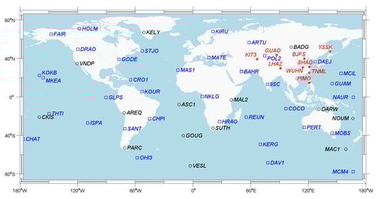
Figure 2.
The core station distribution of SHRRF including 37 ITRF14 core stations (blue square) and nine IGS stations (red asterisk). The black circles mark the 14 abandoned ITRF14 core stations.
3. Stability Analysis of SHRRF
To evaluate the stability of SHRRF, we analyzed the consistency between SHRRF and ITRF14 on the time series of the origin and scale parameters as well as the accuracy of the SHCORS station’s daily solutions.
3.1. Origin and Scale Temporal Behavior
Since the loosely constrained GNSS solutions have large rotational uncertainties, the stability of SHRRF is mainly reflected in the temporal behavior of the origin translations and scale between the different frames [12]. In this section, we analyzed the time series of the origin translations and the scale factor to evaluate the stability of SHRRF, which are shown in Figure 3.
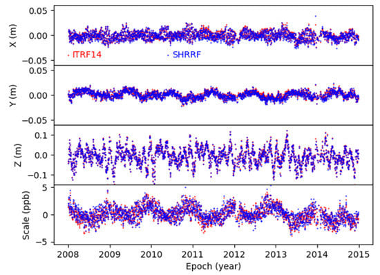
Figure 3.
The temporal variation in the origin translations and scale between SHRRF and ITRF14. The red and blue dots represent the solutions of ITRF14 and SHRRF, respectively.
As shown in Figure 3, under ITRF14, the average standard deviation of the origin translation time series in the X-, Y-, and Z- directions was 0.02, 0.01, and 0.1 m, respectively. The average standard deviation of the scale factor was 4 ppb. The difference between the time series of the transformation parameters under SHRRF and ITRF14 was not significant, meaning that SHRRF performed as well as the most reliable global reference frame co−rotating with the solid Earth. The time series of the origin translations in the Y−direction and the scale factor under ITRF14 and SHRRF showed obvious seasonal signals. This may be due to the “network effect”, which refers to the alignment, implying that the estimation of all seven parameters is highly dependent on the accuracy of the core stations [30,31]. As a consequence, the obvious periodic signal implies the existence of the loading effect, which is not completely modeled out. Further studies are necessary to determine a remedy for the “network effect”.
In summary, there was no significant trend or scatter in all of the origin and scale time series under SHRRF and ITRF14. Since the densification of the SHRRF core stations did not change the temporal behavior of origin and scale, the consistency between SHRRF and ITRF14 was verified.
3.2. The RMSE of SHCORS Instantaneous Solutions
In addition to the Helmert transformation parameters, the root mean square error (RMSE) time series of SHCORS instantaneous solutions are also important factors for SHRRF stability assessment. To evaluate the accuracy of the SHCORS station coordinate under SHRRF, we estimated the average RMSE from the daily solution using the minimum constraints for all of the SHCORS stations at each epoch (denoted as ERMSE) and the average value of RMSE for each site over all epochs (denoted as SRMSE), as follows:
where i and j are indices of the sequence number of epochs and the SHCORS stations, respectively; and n and m are the total number of daily epochs and sites, respectively.
The time series of ERMSE are shown in Figure 4, where the upper, middle, and lower panels show the results of the east, north, and up components, respectively. The differences between ITRF14 and SHRRF were obvious. Most of the ERMSE solutions under SHRRF differed by 1.5 mm in the east and north directions, while the solutions under ITRF14 differed between 1 and 2 mm. Although the ERMSE in the up direction under SHRRF and ITRF14 appeared quite close, with almost 97% of solutions differing by less than 5 mm, the superiority of SHRRF was clear.
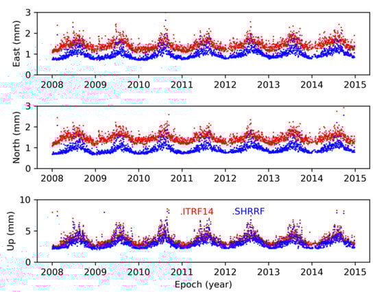
Figure 4.
The distribution plot showing the time series of ERMSE of SHCORS. The ERMSE time series of the SHCORS instantaneous solutions under SHRRF and ITRF14 are shown by blue and red dots, respectively.
Figure 5 shows the SRMSE of all the SHCORS stations calculated by Equation (9). As we can see from the figure, the SRMSE of all sites under SHRRF was significantly reduced in the horizontal direction, by at least 30%, compared to the results under ITRF14. Although the difference in the vertical directions was not large, most of the sites still improved by nearly 10%. This indicates that adding regional stations to the core station network can significantly improve the accuracy in the horizontal direction rather than the vertical direction, which may be affected by more local factors such as the human activities, regional groundwater, and surface water quality migration, etc.
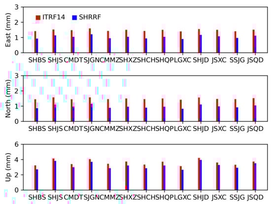
Figure 5.
Bar plots showing the SRMSE of the SHCORS stations. The SRMSE under SHRRF and ITRF14 are indicated by blue bar and red bar, respectively.
4. Applications
4.1. Velocity of SHCORS
Earlier studies have shown that the velocity estimated from a time series shorter than three years was easily affected by the seasonal terms and exhibited a large deviation [32,33]. Therefore, in this section, we only discuss the velocity of nine stations (that is, we excluded JSQD, CMDT, SJGN, and JSXC), the effective continuous observation time spans of which were less than three years. The coordinates, velocity, and nonlinear variations at the reference epoch (2011.0) under SHRRF were calculated through time series analysis. The model of time series analysis is listed as follows:
where is the station coordinates at the reference epoch . represents the station velocity. denotes the amplitude of the seasonal terms. is the amplitude of box function starting from and ending at . denotes the amplitude of post−seismic deformation. is the functional post−seismic deformation model. represents the remaining nonlinear variations.
The blue arrows in Figure 6a represent the horizontal velocity of nine SHCORS stations derived from the coordinate time series under ITRF14, and the red arrows represent the horizontal velocity under SHRRF. The seven−year observations indicate that these nine SHCORS stations moved toward the southeast direction at an average horizontal velocity of 33.6 mm/year. Here, the horizontal velocity is the vector sum of the average velocities in the east and north directions, which was 31.7 and 11.1 mm/year, respectively. The blue arrows in Figure 6b represent the horizontal velocity difference between ITRF14 and SHRRF, which was less than 0.5 mm/year in most cases except for at stations SHJD and SHXZ. SHJD showed the largest differences, reaching 1.1 mm/year.
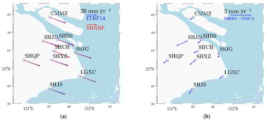
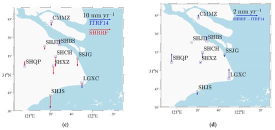
Figure 6.
The spatial distribution and differences of the SHCORS station velocities between SHRRF and ITRF14. (a,b) represents the horizontal velocity, while (c,d) represents the vertical velocity.
The blue and red arrows in Figure 6c indicate the vertical velocities of SHCORS stations under ITRF14 and SHRRF, respectively. Most of the stations are located in the settlement area except for SHBS and SHQP. The station with the largest settlement velocity was SHJS, which reached −6.2 mm/year (under SHRRF) and −5.8 mm/year under ITRF14. The blue arrows in Figure 6d represent the vertical velocity difference between ITRF14 and SHRRF; most were smaller than 0.5 mm/year, except for SHQP and LGXC. The greater vertical velocity difference between SHQP and LGXC may be related to the local groundwater recharge and reclaimed land subsidence.
4.2. Reclaimed Coast−Land Subsidence Study
From 1956 to 2005, 1014 km2 of land was reclaimed in Shanghai to solve the problem of land resource exhaustion [34,35]. The reclaimed area is covered with artificial filling soil, which is very soft, with high water content, large pore ratio, and low strength. Therefore, for a long period after reclamation, the self−weight consolidation of the artificial filling soil or the secondary compression of the silt under the reclaimed soil caused serious surface settlement.
The frequent occurrence of serious land subsidence in the reclaimed area has attracted the attention of many scholars. In order to assess the stability and capacity of building foundations in the reclaimed area, Yang et al. carried out a centrifugal test to study the consolidation phase of the reclaimed soil under self−weight in the east coast of Shanghai [36]. The centrifuge tests used a reduced scale model to recreate the stress conditions that would exist in an actual situation to help solve complex geotechnical problems.
Through these centrifuge tests, a geotechnical empirical model was established. The geotechnical centrifuge model describes the relationship between the cumulative subsidence and the consolidation time (11). This model is a reduced scale numerical model, which can help us to improve our understanding of the basic mechanisms of the reclaimed land deformation, and can be verified by real displacement monitoring data [34].
where indicates the cumulative subsidence assumed at infinite time. k and λ present the model parameters, which are mainly affected by the physical and mechanical properties of the reclaimed soil; and is the cumulative subsidence at the consolidation time .
4.2.1. GNSS Monitoring Network
In order to validate the centrifuge model, a GNSS monitoring network was established in the study area (Figure 7) including one continuously operating reference station LGXC (blue dot) and three semi−permanent (SP) stations SP0018, SP0050, and SPdd21 (red dots). The yellow, red, and blue lines in Figure 7a represent three dams built in 1949, 1983, and 2000, respectively. LGXC is a core station of the SHRRF, located between the 1949 dam and the 1983 dam. SP0018 is located in area A, which was reclaimed before 2000. SP0050 is located in area B, which was reclaimed between 2000 and 2005. SPdd21 is located in the newest reclamation area (area C), which was built between 2006 and 2010. From 13 April 2016 to 15 November 2018, the SP station made 29 observations, with each observation lasting no less than two hours.
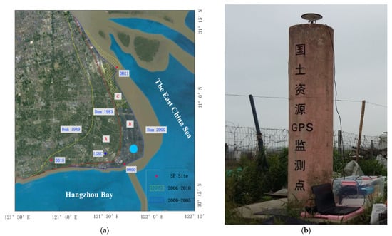
Figure 7.
Photographs depicting the distribution of the GNSS monitoring network in the reclaimed area. (a) shows the distribution of monitoring sites, and (b) is an image of the SP0018 site.
4.2.2. Consolidation Settlement Model under Self−weight
In this section, we used the observations of LGXC to prove the centrifuge model listed in Section 4.2.1 (Equation (11)) and understand the subsidence evolutions of the reclaimed area. The data processing method is described in Section 2. The coordinate solutions of LGXC in the east, north, and up directions relative to different reference frames are exhibited in Figure 8. The constant offset, trend, annual and semiannual terms were subtracted from the time series. We can see that the precision and stability of LGXC relative to SHRRF were better than that of ITRF14.
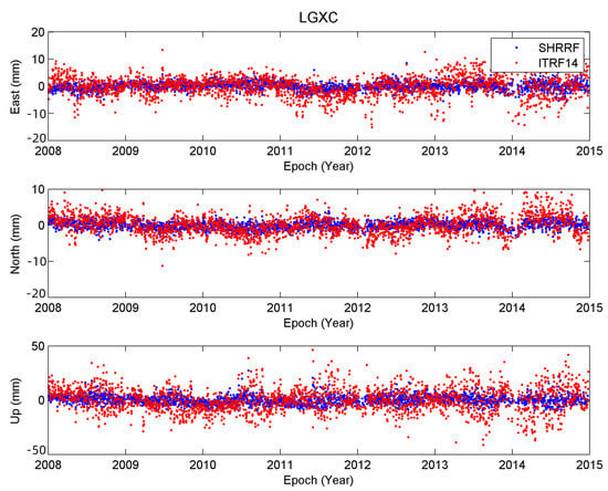
Figure 8.
Distribution plot showing coordinate residual time series of LGXC relative to ITRF14 (blue) and SHRRF (red).
Based on the Levenberg–Marquardt (LM) algorithm, the parameters k and λ in Equation (11) were estimated by using the vertical time series of LGXC. The LM algorithm is an improved algorithm of least squares, which is a nonlinear regression analysis between the Newton iterative method and gradient descent method. The LM algorithm was proposed by K. Levenberg in 1944 [37,38] and verified again by D. W. Marquardt in 1963 [38]. In order for the regularization equation of the LM algorithm to converge quickly in parameter estimation and reduce the computational complexity, we introduced a damping factor in the iteration process.
In this study, only the influence of the gravity of the backfill soil itself was considered; other loads such as the role of the building loading, underground water pumping, etc. were ignored. In addition to this, the deviations of the parameters for different stations in the study area were also ignored. Simultaneously, a time delay factor () was introduced to the model, which indicates the starting time for the consolidation phase of different reclaimed areas. The consolidation settlement model under self−weight for the reclaimed soil in east Shanghai is shown in Equation (12).
4.2.3. Verification of the Consolidation Settlement Model
As shown in Figure 9, the semi−permanent stations SP0018, SP0050, and SPdd21 were used to verify the self−weight consolidation settlement model. The upper panel shows the modeling result of the LGXC station through the LM method. The blue dots are the coordinate solutions of LGXC in the up directions under SHRRF. The red line is the cumulative settlement simulated by the consolidation settlement model from 2008 to 2014, which reached almost 16 mm.
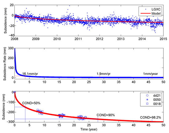
Figure 9.
The distribution plots showing the consolidation settlement model under self−weight.
The middle panel exhibits the change in the subsidence rate over time. The same as that found by Yang et al. in the laboratory through a centrifugation experiment [36], the settlement of the alluvial deposit creep of the reclamation fill could be distinguished into three phases: the quick, primary, and slow consolidation phases. In the quick and primary consolidation phases, the subsidence rate was greater than 16.1 mm/year, and between 16.1 and 1 mm/year, respectively. When the subsidence velocity was lower than 1.9 mm/year, it entered the slow consolidation phase.
The red line in the lower panel represents the change in the cumulative subsidence over time, which is extended by the red line in the upper panel. The blue squares, asterisks, and circles represent the vertical time series of the semi−permanent stations SP0018, SP0050, and SPdd21, respectively. In the quick consolidation phase, soil settled fast and 50% of the subsidence took place during the first 3.6 years. A total of 90% of the total subsidence was completed during the primary consolidation phase, which took about 28.4 years. After 46.4 years, when the subsidence velocity was lower than 1 mm/year, we can assume that the subsidence has basically ceased.
As shown in the lower panel of Figure 9, all three SP observations fit the model well. Stations SP0018 and SP0050 of reclamation areas A and B, respectively, are currently at the end of the primary consolidation phase and can be expected to enter the slow consolidation phase within four years after the last observation (2018.8). Excluding the effects of loading other than that of self−weight, the total subsidence in these areas will not exceed 20 mm before the subsidence ceases (basically, the subsidence velocity is less than 1 mm/year). At present, the consolidation degree of area C is only 56%, which is still in the primary consolidation phase, and the subsidence rate is relatively high, up to 22 mm/year. It is expected that after 18 years (2018.8), it will enter the slow consolidation phase, and the total settlement will exceed 100 mm. In order to compare the difference between the observations and the consolidation settlement model under different frames, we calculated the standard deviation between the SP stations’ observed values and simulated values of the model under ITRF14 and SHRRF. As shown in Table 3, the deviations of all of the SP stations under ITRF14 were greater than SHRRF. All of the standard deviations associated with SHRRF were less than 10 mm, while the maximum standard deviation under the ITRF14 framework reached 30.8 mm (0050).
Table 3.
The standard deviations between the SP stations’ observed values and the consolidation settlement model under different frames.
5. Conclusions
In this work, the stable regional densified reference frame in Shanghai, East China (SHRRF) was implemented with the following objectives: to monitor the current situation of land subsidence in reclamation areas; characterize and gain insights of the present and future evolution of reclaimed coast–land subsidence; and provide a basis for regional disaster prevention and urban planning.
SHRRF was aligned to ITRF14 by seven frame parameters of transformation through a set of well−distributed core stations, in order to preserve the frame stability and the internal solution structure of the regional sub−network. The core station network includes 37 well−distributed ITRF14 frame stations, nine IGS stations in and around China, and six SHCORS stations. SHRRF provides a precise regional reference frame. The consistency of the origin and scale parameters of the time series between SHRRF and ITRF14 proves the stability of SHRRF. The comparison results of the RMSE time series and the average RMSE for all of the local stations under different frameworks illustrate the superiority of SHHRF, indicating that a millimeter−accuracy position time series could be easily obtained underlying this regional frame.
Based on the high precision permanent GNSS vertical solutions under SHRRF and a geotechnical centrifuge model, a temporal consolidation settlement model of the reclaimed soil, under self−weight in East China, was established. The well−fitted settlement model indicates that the total subsidence of the reclaimed soil should require more than 46 years. Approximately 50% of the subsidence should occur in about 4 years, with 90% of the total subsidence basically occurring within 29 years. Area C of the study area was determined to be the most dangerous region; thus, it will require stricter monitoring, and the public facilities and infrastructure should be carefully laid out in this area.
Finally, the consolidation settlement model established in this work mainly considered the effect of the reclaimed soil self−weight. If other loading factors are taken into account such as building loads and variation of water mass, it would be expected for the consolidation process to potentially be shorter and the total settlement to be greater. In future research, we plan to integrate various influential loading factors to build a consolidation settlement model, which is more adaptable for coast–land regional planning, safety maintenance, and disaster prevention.
Author Contributions
Conceptualization and methodology, D.D.; Software, D.D. and Y.P.; Formal analysis, C.Z.; Investigation, Y.P. and C.Z.; Resources, W.C. and Y.P.; Data curation, Y.P.; Writing—original draft preparation, Y.P.; Writing—review and editing, Y.P. and W.C.; Visualization, C.Z.; Validation, D.D. and W.C.; Project administration, W.C.; Funding acquisition, W.C. All authors have read and agreed to the published version of the manuscript.
Funding
This work was sponsored by the National Natural Science Foundation of China (No. 41771475); the Social Development Project of Science, Technology Innovation Action Plan of Shanghai (No. 20dz1207107); the Fund of Director of Key Laboratory of Geographic Information Science (Ministry of Education), the East China Normal University (No. KLGIS2017C01); the Fundamental Research Funds for the Central University (No. 40500−20104−222235); and Research Funds of East China Normal University (No. 40500-20104-222460).
Acknowledgments
We are grateful to the Shanghai Surveying and Mapping Institute for providing the GNSS observations.
Conflicts of Interest
The authors declare no conflict of interest.
References
- Yu, L.; Yang, T.; Zhao, Q.; Liu, M.; Pepe, A. The 2015–2016 Ground Displacements of the Shanghai Coastal Area Inferred from a Combined COSMO−SkyMed/Sentinel−1 DInSAR Analysis. Remote Sens. 2017, 9, 1194. [Google Scholar] [CrossRef]
- Shen, S.L. Geological environmental character of Lin Gang New City and its influences to the construction. Shanghai Geol. 2008, 105, 24–28. (In Chinese) [Google Scholar]
- Xu, J.J.; Chen, Y. Research on reclamation of Nanhui Dongtan Based on RS and GIS. Shanghai Land Resources 2011, 32, 18–22. (In Chinese) [Google Scholar]
- Tosi, L.; Teatini, P.; Carbognin, L.; Frankenfield, J. A new project to monitor land subsidence in the northern Venice coastland (Italy). Environ. Geol. 2007, 52, 889–898. [Google Scholar] [CrossRef]
- Cenni, N.; Viti, M.; Baldi, P.; Mantovani, E.; Vannucchi, A. Present vertical movements in Central and Northern Italy from GPS data: Possible role of natural and anthropogenic causes. J. Geodyn. 2013, 71, 74–85. [Google Scholar] [CrossRef]
- Avsar, N.B.; Jin, S.G.; Kutoglu, H.; Gürbüz, G. Vertical Land Motion Along the Black Sea Coast from Satellite Altimetry, Tide Gauges and GPS. Adv. Space Res. 2017, 60, 2871–2881. [Google Scholar] [CrossRef]
- Floris, M.; Fontana, A.; Tessari, G.; Mulè, M. Subsidence Zonation Through Satellite Interferometry in Coastal Plain Environments of NE Italy: A Possible Tool for Geological and Geomorphological Mapping in Urban Areas. Remote Sens. 2019, 11, 165. [Google Scholar] [CrossRef]
- Blackwell, E.; Shirzaei, M.; Ojha, C.; Werth, S. Tracking California’s sinking coast from space: Implications for relative sea−level rise. Sci. Adv. 2020, 6, eaba4551. [Google Scholar] [CrossRef]
- Zhou, X.; Wang, G.; Wang, K.; Liu, H.; Lyu, H.; Turco, M.J. Rates of Natural Subsidence along the Texas Coast Derived from GPS and Tide Gauge Measurements (1904–2020). J. Surv. Eng. 2021, 147, 04021020. [Google Scholar] [CrossRef]
- Haley, M.; Ahmed, M.; Gebremichael, E.; Murgulet, D.; Starek, M. Land Subsidence in the Texas Coastal Bend: Locations, Rates, Triggers, and Consequences. Remote Sens. 2022, 14, 192. [Google Scholar] [CrossRef]
- Bosy, J. Global, Regional and National Geodetic Reference Frames for Geodesy and Geodynamics. Pure Appl. Geophys. 2014, 171, 783–808. [Google Scholar] [CrossRef]
- Altamimi, Z.; Boucher, C.; Sillard, P. Terrestrial reference frame requirements within GGOS perspective. J. Geodyn. 2005, 40, 363–374. [Google Scholar] [CrossRef]
- Altamimi, Z.; Collilieux, X.; Legrand, J.; Garayt, B.; Boucher, C.; Sillard, P. ITRF2005: A new release of the International Terrestrial Reference Frame based on time series of station positions and Earth Orientation Parameters. J. Geophys. Res. Solid Earth 2007, 112, B09401. [Google Scholar] [CrossRef]
- Rebischung, P.; Griffiths, J.; Ray, J.; Schmid, R. IGS08: The IGS realization of ITRF2008. GPS Solut. 2012, 16, 483–494. [Google Scholar] [CrossRef]
- Blewitt, G.; Kreemer, C.; Hammond, W.; Goldfarb, J.M. Terrestrial Reference Frame NA12 for crustal deformation studies in North America. J. Geodyn. 2013, 72, 11–24. [Google Scholar] [CrossRef]
- Altamimi, Z.; Boucher, C.; Sillard, P. New trends for the realization of the international terrestrial reference system. Adv. Space Res. 2002, 30, 175–184. [Google Scholar] [CrossRef]
- Sanchez, L.; Drewes, H. Crustal deformation and surface kinematics after the 2010 earthquakes in Latin America. J. Geodyn. 2016, 102, 1–23. [Google Scholar] [CrossRef]
- Mazurova, E.M.; Sergei, K.; Aleksandr, K. Development of a terrestrial reference frame in the Russian Federation. Stud. Geophys. Geod. 2017, 61, 616–638. [Google Scholar] [CrossRef]
- Wang, G.; Kearns, T.J.; Yu, J.B.; Saenz, G. A stable reference frame for landslide monitoring using GPS in the Puerto Rico and Virgin Islands region. Landslides 2014, 11, 119–129. [Google Scholar] [CrossRef]
- Wang, G.; Bao, Y.; Gan, W.; Geng, J.; Xiao, G.; Shen, S.L. NChina16: A stable geodetic reference frame for geological hazard studies in North China. J. Geodyn. 2018, 115, 10–22. [Google Scholar] [CrossRef]
- Bertiger, W.; Desai, S.D.; Haines, B.; Harvey, N. Single receiver phase ambiguity resolution with GPS data. J. Geod. 2010, 84, 327–337. [Google Scholar] [CrossRef]
- Dong, D.; Fang, P.; Bock, Y.; Cheng, M.K. Anatomy of apparent seasonal variations from GNSS derived site position time series. J. Geophys. Res. 2002, 107, 9–16. [Google Scholar]
- Nikolaidis, R. Observation of Geodetic and Seismic Deformation with the Global Positioning System. Ph.D. Thesis, University of Calif, San Diego, CA, USA, 2002. [Google Scholar]
- Montillet, J.P.; Bos, M.S. Geodetic Time Series Analysis in Earth Sciences; Springer Geophysics: Berlin/Heidelberg, Germany, 2019; pp. 30–35. [Google Scholar]
- Dong, D.; Fang, P.; Bock, Y.; Webb, F.H. Spatiotemporal filtering using principal component analysis and Karhunen−Loeve expansion approaches for regional GPS network analysis. J. Geophys. Res. Solid Earth 2006, 111, B03405. [Google Scholar] [CrossRef]
- Dong, D.; Yunck, T.; Heflin, M. Origin of the International Terrestrial Reference Frame. J. Geophys. Res. Solid Earth 2007, 108, 2200. [Google Scholar] [CrossRef]
- Altamimi, Z.; Collilieux, X.; Métivier, L. ITRF2008: An improved solution of the international terrestrial reference frame. J. Geod. 2011, 85, 457–473. [Google Scholar] [CrossRef]
- Altamimi, Z.; Rebischung, P.; Métivier, L.; Collilieux, X. ITRF2014: A new release of the International Terrestrial Reference Frame modeling nonlinear station motions. J. Geophys. Res. Solid Earth 2016, 8, 6109–6131. [Google Scholar] [CrossRef]
- Sillard, P.; Boucher, C. A review of algebraic constraints in terrestrial reference frame datum definition. J. Geod. 2001, 75, 63–73. [Google Scholar] [CrossRef]
- Collilieux, X.; Dam, T.V.; Ray, J.; Coulot, D.; Métivier, L.; Altamimi, Z. Strategies to mitigate aliasing of loading signals while estimating GPS frame parameters. J. Geod. 2012, 86, 1–14. [Google Scholar] [CrossRef]
- Blewitt, G.; Lavallée, D. Effect of annual signals on geodetic velocity. J. Geophys. Res. Solid Earth 2010, 107, ETG 9-1–ETG 9-11. [Google Scholar] [CrossRef]
- Bennett, R.A.; Hreinsdottir, S. Constraints on vertical crustal motion for long baselines in the central Mediterranean region using continuous GPS. Earth Planet. Sci. Lett. 2007, 257, 419–434. [Google Scholar] [CrossRef]
- Klos, A.; Olivares, G.; Teferle, F.N.; Hunegnaw, A.; Bogusz, J. On the combined effect of periodic signals and colored noise on velocity uncertainties. GPS Solut. 2018, 22, 1. [Google Scholar] [CrossRef]
- Zhao, Q.; Pepe, A.; Gao, W.; Zhong, L. A DInSAR Investigation of the Ground Settlement Time Evolution of Ocean−Reclaimed Lands in Shanghai. IEEE J. Sel. Top. Appl. Earth Obs. Remote Sens. 2015, 8, 1763–1781. [Google Scholar] [CrossRef]
- Ding, J.Z.; Zhao, Q.; Tang, M.C.; Calò, F.; Zamparelli, V.; Falabella, F.; Liu, M.; Pepe, A. On the Characterization and Forecasting of Ground Displacements of Ocean−Reclaimed Lands. Remote Sens. 2020, 12, 2971. [Google Scholar] [CrossRef]
- Yang, P.; Tang, Y.Q.; Zhou, N.Q. Consolidation settlement of Shanghai dredger fill under self−weight using centrifuge modeling test. Cent. South Univ. Technol. 2008, 39, 862–866. (In Chinese) [Google Scholar]
- Levenberg, K. A Method for the Solution of Certain Problems in Least Squares. Int. J. Numer. Method Biomed Eng. 1944, 2, 164–168. [Google Scholar]
- Marquardt, D.W. An Algorithm for Least−Squares Estimation of Nonlinear Parameters. J. Soc. Ind. Appl. Math. 1963, 11, 431–441. [Google Scholar] [CrossRef]
Publisher’s Note: MDPI stays neutral with regard to jurisdictional claims in published maps and institutional affiliations. |
© 2022 by the authors. Licensee MDPI, Basel, Switzerland. This article is an open access article distributed under the terms and conditions of the Creative Commons Attribution (CC BY) license (https://creativecommons.org/licenses/by/4.0/).