Abstract
Due to the conservation of global angular momentum, polar motion (PM) is dominated by global mass redistributions and relative motions in the atmosphere, oceans and land water at seasonal time scales. Thus, accurately measured PM data can be used to validate the general circulation models (GCMs) for the atmosphere, oceans and land water. This study aims to analyze geophysical excitations and observed excitations obtained from PM observations from both the harmonic and wavelet analysis perspectives, in order to refine our understanding of the geophysical excitation of PM. The geophysical excitations are derived from two sets of GCMs and a monthly gravity model combining satellite gravity data and some GCM outputs using the PM theory for an Earth model with frequency-dependent responses, while the observed excitation is obtained from the PM data using the frequency-domain Liouville’s equation. Our results show that wavelet analysis can reveal the time-varying nature of all excitations and identify when changes happen and how strong they are, while harmonic analysis can only show the average amplitudes and phases. In particular, the monthly gravity model can correct the mismodeled GCM outputs, while the Earth’s frequency-dependent responses provide us with a better understanding of atmosphere–ocean–land water–solid Earth interactions.
1. Introduction
The Earth Orientation Parameters (EOPs), namely nutation, polar motion (PM) and changes in universal time ΔUT1, are essential in the coordinate transformations between the geocentric celestial reference frame (GCRF) and the international terrestrial reference frame (ITRF) [1].
While nutation can be accurately modeled by the IAU2000A nutation model, real-time PM and ΔUT1 are not available, mainly due to delays in collecting and processing global data sets, and therefore accurate and efficient prediction of EOPs is urgently needed for a number of real-time practical applications, such as precise positioning, satellite navigation and satellite orbit determination [1,2,3,4,5,6]. However, why is it necessary to investigate the geophysical excitations of PM and ΔUT1? The reasons are listed below:
- PM and ΔUT1 are dominated by mass redistributions and relative motions in the atmosphere, oceans and land water (due to conservation of angular momentum) from subdaily to seasonal time scales and beyond;
- The general circulation models (GCMs) of the atmosphere, ocean and hydrology, developed by different institutes, can provide forecast products, including mass redistributions and motions in the atmosphere, oceans and land water (see below and Section 3 for more details about GCM products);
- Predictions of PM and ΔUT1 can be improved using forecasts of atmospheric, oceanic and hydrological excitations if they agree well with the existing PM and ΔUT1 observations;
- Relying on accurately measured EOP data, the quality of GCM outputs can be also checked and improved.
Relying on accurately measured EOP data, the quality of GCM outputs can be also checked and improved.
According to the above reasons, it is of great significance to study atmospheric, oceanic and hydrological excitations (respectively denoted as AE, OE and HE) of PM and ΔUT1. This study focuses only on the excitations of seasonal PMs, which are dominated by mass redistributions and relative motions in the atmosphere, oceans and land water [3,7,8,9,10,11,12].
Based on the GCMs of the atmosphere developed by different institutes, a number of studies explored the contributions of atmospheric wind and pressure fluctuations to the annual component of PM and showed that it is mainly due to the annual appearance of a high-atmospheric-pressure system over Siberia every winter [7,8,9,10,11,12,13,14,15,16]. These studies also proved that although the agreement between observations and atmospheric excitation is rather good for the prograde annual amplitude, the agreements for other seasonal terms (such as the semi-annual and ter-annual wobbles) are poor. Therefore, there must be some other processes contributing to the excitations of seasonal wobbles.
With the development of GCMs for oceans and land water, many studies have shown that including nontidal oceanic excitation besides the atmospheric one can bring better agreement with the observed excitation [12,17,18,19,20,21,22,23]. Additional studies also proved that the contributions of hydrological processes (soil moisture and snow load) should not be ignored in exciting the annual and semiannual wobbles, though there are large errors in the hydrological models [24,25,26,27,28].
More recently, self-consistent atmospheric, oceanic and hydrological excitations derived from GCM outputs, such as the ESMGFZ effective angular momentum (EAM) products, became available and improved their agreement with the observations significantly [29]. However, large discrepancies still exist between the modeled and observed PM excitations [30,31,32], partly due to the fact that the conservation of global mass is violated when combining these GCM outputs [32,33].
While most previous studies on the seasonal PM excitation rely on harmonic analyses, a few also used wavelet analyses to reveal the inharmonic nature of the seasonal PM excitations. Using the normal Morlet wavelet transform analysis, Liu et al. [34] showed that atmospheric pressure and oceanic currents play the most significant and stable role in exciting annual PM. Chao et al. [35] analyzed PM excitation for the period 1900–2012 using wavelet analysis, found an ~8-year quasi-periodic signal and proved the existence of the ~26-year Markowitz wobble. Besides PM excitation, Luo et al. [36] also applied wavelet analysis to the excitation of length-of-day (LOD) variations and found that consideration of wavelet-based inharmonic excitation can achieve a better match with the observed LOD time series.
Satellite Laser Ranging (SLR) is a method to measure the distance to satellites by using very short laser pulses; it has been used to monitor changes in the degree-2 zonal harmonics C20 for more than four decades [37,38,39] and has been extended to estimates of other low-degree harmonics in recent years [40,41]. The 2002 launch of the Gravity Recovery and Climate Experiment (GRACE) twin satellites made available several time series of geopotential coefficients [42,43,44,45,46,47,48,49], which can provide information for surficial mass redistributions with much higher spatial resolution. Therefore, SLR and GRACE provide us with a much better understanding of mass redistributions on the global scale and matter-term excitations meeting the conservation of global mass. Notable discrepancies are found between GCM-based and SLR/GRACE-based PM excitations [32,33,50].
Despite the advantages of GRACE data over the period for which it is available, there are also some significant defects in the GRACE-based excitations. Due to the longitudinal striped errors of traditional GRACE spherical harmonic products, additional corrections (destriping and smoothing) are required to reveal valuable signals [51,52,53]. While mass redistributions derived by different researchers can differ from each other with the different GRACE data processing strategies adopted, destriping would cause distortions of signals of interest, while smoothing would attenuate them (signal leakages) [52,53]. These problems make the GRACE-based results not quite reliable. The newly released Mascon products are free of the longitudinal striped errors but also contain some problems. As pointed out by Chen et al. [33], atmospheric, oceanic and hydrological model outputs (used to generate the RL06 AOD1B) violate the conservation of global mass, so a sea-level mass term is introduced to conserve the mass; however, only the ocean model outputs are used to produce the RL06 GAB (namely, parts of oceanic contributions are not modeled). In addition, as with traditional GRACE spherical harmonic products, there are notable differences among Mascon products released by different institutes (more details can be found in [33]). Thus, further improvements are needed for GRACE products.
Chen et al. [33] developed a multiple-data-combined monthly gravity model set LDCmgm90 (available at https://doi.org/10.6084/m9.figshare.7874384.v4 (accessed on 20 January 2022)) by assimilating various versions of GRACE (including Mascon products), SLR monthly gravity data [38,39,40,41] and outputs from different global atmospheric, oceanic and hydrological circulation models, by using the least difference combination (LDC) method proposed by Chen et al. [32,54]. The LDC is a method developed in the frequency domain and can adequately address both the magnitude and phase aspects simultaneously when combining different data, even for the trends and very-low frequency components of data (more details can be found in [54]). Therefore, the LDCmgm90 data set can provide more reliable data trends and seasonal signals and has no stripes, as seen in most GRACE data, and it was shown to have better performance in explaining atmospheric, oceanic and hydrological long-term and seasonal time-scale mass redistributions compared with most meteorological models and time-varying gravity products, including Mascon solutions (see [32,33,55,56] for validations of LDCmgm90 from different aspects).
On the other hand, Chen et al. [57] developed a new PM excitation theory for an Earth model with the effects of mantle anelasticity, quasi-fluid rheology, dynamic ocean tides and ocean pole tides, and they showed that the geophysical excitations of PM are frequency-dependent (see Appendix B). Chen et al. [32,54] and Ding and Chao [58] validated the frequency-dependent response model and showed that using the new theory can improve the agreement between geophysical and observed excitations. Chen et al. [33] also provided the improved global angular momentum data LDCgam (https://doi.org/10.13140/RG.2.2.28698.49604, (accessed on 20 January 2022)), corresponding to LDCmgm90 and using the PM excitation theory with frequency-dependent responses.
While harmonic analysis and PM theory with constant responses are the de facto standards in PM excitation studies, in this research, we aim to refine our understanding of geophysical excitations and the observed PM, relying on both GCM-based and satellite gravimetry-based excitations, from both harmonic and inharmonic approaches, and using both PM theories with constant and frequency-dependent responses. This study will show that the PM theory with frequency-dependent responses and some inharmonic analyses (such as wavelet analysis) are more suitable for PM excitation studies.
2. Materials and Methods
2.1. Data
Various data sets are needed in order to study the seasonal excitations of PM, and they are collectively listed in Table 1 and described in the following subsections. Only the data sets numbered with Arabian numbers in the following subsections are adopted by this study, although many other sets of data/models are mentioned below to describe them.

Table 1.
Data sets adopted by this study.
2.1.1. Polar Motion and Observed Excitation
ITRF2020 is the latest realization of the International Terrestrial Reference System based on completely reprocessed time series of station positions and EOPs provided by the Technique Centers of Very Long Baseline Interferometry (VLBI), Global Navigation Satellite System (GNSS), SLR and Doppler Orbitography and Radio-Positioning Integrated by Satellite instrument (DORIS), as well as local ties at colocation sites [59].
PM reflects the time-dependent coordinates of the Earth’s reference axis (currently the celestial intermediate pole) with respect to the ITRF. The coordinate x is measured along the 0° (Greenwich) meridian, while the coordinate y is measured along the 90°W meridian. As a part of the ITRF2020 solutions, the ITRF2020 PM time series (available at https://itrf.ign.fr/ftp/pub/itrf/itrf2020/ITRF2020_EOP-F1.DAT; accessed on 18 April 2022) is certainly the best choice. Thus, we have the following.
- 1.
- PM from the ITRF2020 files. PM can be described as p(t) = x(t) − iy(t), where x and y are daily-sampled in milli-arcsecond (mas). The observed excitation can be obtained from PM data by using Equation (A3). See Figure 1a for plots of time series of PM and Figure 1b for plots of time series of observed excitation.
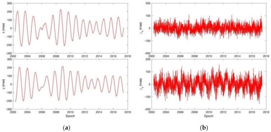 Figure 1. Time series for the observed PM and the geodetic excitation. (a) The x- and y-components of PM; (b) the x- and y-components of the geodetic excitation derived from the observed PM using Equation (A3).
2.1.2. General Circulation Models and Angular Momentum Data
Various GCMs of the atmosphere, ocean and hydrology were developed by different institutes. Those to be used in this study are briefly described below.
- The NCEP/NCAR (National Centers for Environmental Prediction/National Center for Atmospheric Research) atmosphere model is based on the conservation of mass, energy and moisture, with the conservation of momentum replaced by the vorticity and divergence equations, which takes advantage of the spectral technique in the horizontal and eliminates the difficulties associated with the spectral representation of vector quantities on a sphere [60,61].
- The ECCO (Estimating the Circulation and Climate of the Ocean) ocean model run at JPL is based on the MIT-GCM (Massachusetts Institute of Technology General Circulation Model) and driven by the surface wind stress, heat and freshwater fluxes (but no surface pressure) from the NCEP reanalysis, and thus the ECCO ocean model is consistent with the NCEP atmosphere model [62].
- The ECMWF (European Centre for Medium-Range Weather Forecasts) atmosphere model is based on equations similar or equivalent to those used by NCEP, but adopts different diagnostic equations that give the static relation between different model parameters. The NCEP model uses the vertical velocity equation obtained from the continuity equation discretized in the vertical, while the ECWMF model uses the gas law providing the relation between pressure, density and temperature [63].
- The Max Planck Institute Ocean Model (MPIOM) includes an embedded dynamic/thermodynamic sea ice model with a viscous–plastic rheology and a bottom boundary layer scheme for the flow across steep topography, under the hydrostatic and Boussinesq assumptions [64]. The version used here is forced by both surface wind stress and pressure derived from ECMWF.
- The Land Surface Discharge Model (LSDM) simulates the global vertical and lateral water transport and storage on land surfaces and provides large-scale continental water mass transport processes and storage compartments (soil moisture, snow, rivers and lakes, runoff, drainage) [65,66]. The adopted version is also forced by precipitation, evaporation and temperature derived from ECMWF.
Relying on these GCMs and taking into account the self-consistencies among them, we decide to use the GCM-derived angular momenta as grouped below (see Figure 2).
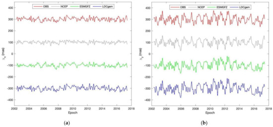
Figure 2.
Time series of observed and geophysical excitations. (a) x-components; (b) y-components. The means, trends and high-frequency components (higher than 6 cycles per year) are removed for all series. These series are shifted vertically for better visibility.
- 2.
- NCEP AE [16,67] + ECCO OE [62] (hereafter NCEP for short). The AE data derived from the NCEP/NCAR reanalysis (available at http://files.aer.com/aerweb/AAM/ (accessed on 20 January 2022)) are used in this study. The OE data from the ECCO kf80i run are adopted, as the kf80i run has assimilated sea surface height data and removed the tidal contamination present in previous versions of the ECCO data (see [62] for details; available at https://isdc.gfz-potsdam.de/ggfc-oceans/oam/ (accessed on 20 January 2022)). Since the ECCO model is not forced by atmospheric surface pressure from the NCEP reanalysis, it is usual to assume the inverted barometer (IB) model to account for the effects of atmospheric pressure over the oceans when using the ECCO ocean model. The IB model is a realistic approximation of the oceans’ response to surface pressure variations at seasonal time scales [68].
- 3.
- ESMGFZ AE + OE + HE + SLE (sea-level excitation) [69] (hereafter ESMGFZ for short). The Earth System Modelling group at Deutsches GeoForschungsZentrum (ESMGFZ) provides 3-h-sampled data for AE and OE, as well as daily-sampled HE and SLE. The AE is derived from the European Centre for Medium-Range Weather Forecasts (ECMWF) model, the OE is obtained from the Max Planck Institute for Meteorology Ocean Model (MPIOM) and the HE is calculated according to the Land Surface Discharge Model (LSDM). The additional product SLE is introduced to conserve global mass. These data are collectively termed ESMGFZ data sets and can be downloaded at http://rz-vm115.gfz-potsdam.de:8080/repository (accessed on 20 January 2022).
These geophysical excitations are to be compared with the excitations derived from the observed PM and LDCmgm90.
2.1.3. LDCmgm90 and LDCgam Data
LDCmgm90 is a monthly gravity model set derived from various GRACE/SLR monthly gravity + various GCM outputs + EOP measurement constraints using the LDC method. The LDCmgm90, complete from degree and order 2 to 90, has the same functions as the GRACE monthly gravity model sets as released by different institutes, such as the Center for Space Research (CSR), Deutsches GeoForschungsZentrum (GFZ), Jet Propulsion Laboratory (JPL) and Graz University of Technology (TUG), but with improved performance compared to traditional GRACE monthly gravity data (see [32,33] for more details).
The GRACE monthly gravity products (termed GSM) are usually released together with the GRACE AOD1B products, which provide a model-based data set (including GAA, GAB, GAC and GAD) that describes the time variations of the gravity potential at satellite altitudes that are caused by nontidal mass redistributions in the atmosphere and oceans [70]. While the GAA product refers to the monthly nontidal atmospheric mass anomalies simulated by the operational run of the atmosphere model ECMWF, the GAB describes monthly nontidal oceanic mass anomalies simulated by the operational run of the (unconstrained) ocean model MPIOM. The GAC is the sum of GAA and GAB, and the GAD can be regarded as a revised version of GAC with nontidal atmospheric and oceanic mass anomalies only over ocean areas. GSM is simply the gravity residual after GAA and GAB are removed from the GRACE observations. The AOD1B products are released by ESMGFZ and adopted by all teams that release GRACE data. The latest versions of these data are RL06 ones (RL06 means release 06).
By analyzing the round-trip distances between the ground and Starlette, Ajisai, Stella, LAGEOS-1 and LAGEOS-2 satellites, the Center for Space Research (CSR) of the University of Texas (UT) at Austin provides low-degree monthly Stokes coefficients (available at http://download.csr.utexas.edu/pub/slr/degree_5/ (accessed on 20 January 2022)). There is a clear improvement in the estimates starting in early 2012, when the sixth satellite (LARES) becomes available. The SLR can provide low-degree zonal harmonics, such as C20 and C30, with higher reliability than the low-altitude GRACE satellites do [37,38,39,40,41].
As with the monthly GRACE gravity models, the LDCmgm90 data set also has five components, namely the GSM, GAA, GAB, GAC and GAD products. However, unlike common GRACE solutions, destriping correction is not used in processing LDCmgm90 solutions, which do not contain stripe errors. The LDCmgm90 GSM data set provides Stokes coefficients for degree/order 2~90. Plots of the LDCmgm90 low-degree Stokes coefficients, compared with the GRACE/SLR solutions provided by the above-mentioned institutes, are given in Figure 3, from which the advantages of LDCmgm90 are apparent.
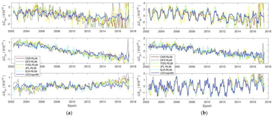
Figure 3.
Stokes coefficients C20, C21 and S21 from different sources (from [33] with the authors’ permission). (a) GSM data for 163 months (no interpolation applied); (b) GSM + GAA + GAB data with cubic spline interpolations for better displays of seasonal cycles. The means of all series are removed. Reproduced with permission from Wei Chen, Scientific Data; published by Springer Nature, 2019.
Relying on Equations (A10)–(A12) in Appendix C, one can obtain the matter-term excitations from the LDCmgm90 degree-2 Stokes coefficients. Further, we adopt the corresponding motion terms derived from the LDC method [32]. Thus, we have the data set:
- 4.
- LDCgam AE + OE + HE. Here, HE is not strictly hydrological but contains some small yet non-negligible effects, such as cryospheric changes.
The LDCgam data used in this study are available at https://doi.org/10.13140/RG.2.2.28698.49604 (accessed on 20 January 2022).
2.2. Method
2.2.1. Harmonic Analysis
Harmonic analysis is a mathematical method for describing and analyzing signals of a periodically recurrent nature. If a function f(t) is single-valued and continuous except for a finite number of discontinuities of the first kind, and has only a finite number of extremums in a period (namely the Dirichlet conditions), it can be represented in the form of an integration
or expanded in the form of the sum of an infinite number of exponential sums, which is more suitable for numerical calculations.
For the case of PM excitation, the expression may be written as [3]
where and are the amplitude and phase angle of the component with angular frequency , and the subscripts p and r denote prograde and retrograde, respectively. In the context of this study, σ can be biennial, annual or semi-annual frequency.
2.2.2. Wavelet Analysis
If the term exp(−iσt) is replaced by a wavelet function in Equation (1), we then obtain the wavelet transformation [71]
where a and τ are timescale and time translate, respectively, while is the conjugate of . The wavelet transform can be viewed as the sum over all time of the signal multiplied by scaled, shifted versions of , and thus each wavelet coefficient is a function of scale and position.
While the base function is unique for harmonic analysis, there are a large number of wavelets (grouped as wavelet families) that one can choose. Wavelet families vary in terms of several important properties [71]:
- Support of the wavelet in time and frequency and rate of decay.
- Symmetry or antisymmetry of the wavelet. The perfect reconstruction filters for symmetric or antisymmetric wavelets have a linear phase.
- Number of vanishing moments. Wavelets with large vanishing moments result in sparse representations for signals.
- Regularity of the wavelet. The adoption of smoother wavelets can provide sharper frequency resolution and lead to faster convergence in iterative algorithms for wavelet constructions.
- Existence of a scaling function.
The only compactly supported, orthogonal and symmetric wavelet is the Haar wavelet, or the Daubechies wavelet of order 1, db1 (thus, Haar has a linear phase). No other compactly supported, orthogonal wavelet can be symmetric. However, there are some wavelets (such as the Symlets and Coiflets) that are nearly symmetric, meaning that their phases are almost linear. In particular, the Coeflets are compactly supported, orthogonal wavelets with the highest number of vanishing moments for both wavelet and scaling functions for a given support width, though there are no analytical expressions for the Coeflets. Thus, the Coeflets are very suitable for the current case, which deals with quasi-periodic seasonal excitations of PM. The Coeflet wavelet of order 5, coif5, is adopted in this study since it has the largest support width (see Figure 4 for the coef5 wavelet function) in the Coeflet family. Other symmetric or nearly symmetric wavelets (such as the Mexician hat wavelet) can also be used, leading to slightly different results that will not alter our conclusions. Further, for the purpose of illustrating the weakness of the (de facto standard) harmonic analysis, it is better to compare the selected time series of harmonic frequency components with the wavelet-based quasi-periodic time series with corresponding scales (rather than the wavelet time–frequency spectrum; also note that the wavelet scale is analogous to the harmonic period), as will be shown in Section 3.
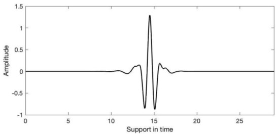
Figure 4.
The coif5 wavelet function.
3. Results
Due to the quasi-periodic seasonal heating from the Sun, caused by the Earth’s orbit around the Sun and the Earth’s axial tilt relative to the ecliptic plane, the atmosphere and oceans exhibit rather strong changes at seasonal frequencies. Here, we focus mainly on the quasi-biennial, annual and semi-annual ones.
On the basis of the theory presented in the Appendix A, Appendix B and Appendix C and the method and data described in Section 2, we have obtained the harmonic and inharmonic PM excitations for the quasi-biennial, annual and semi-annual periods, which are illustrated in the following subsections.
3.1. Seasonal Excitations
3.1.1. Quasi-Biennial Components
The quasi-biennial oscillation (QBO) is a quasi-periodic oscillation of the equatorial zonal wind between easterlies and westerlies in the tropical stratosphere with variable amplitude and period (the mean period is ~28 months) [72]. The QBO would cause quasi-biennial fluctuations in AAM and thus can excite a quasi-biennial PM.
The quasi-biennial PM excitations for all four data sets obtained from both harmonic and wavelet analyses are displayed in Figure 5.
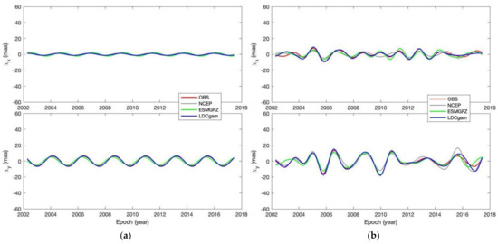
Figure 5.
Quasi-biennial PM excitations. (a) Harmonic fitting according to Equation (2); (b) wavelet analyses based on the coif5 wavelet, as shown in Figure 4.
3.1.2. Annual Components
As the most significant seasonal signal, annual components dominate the changes in almost all the layers of the atmosphere and oceans.
The annual PM excitations for all four data sets obtained from both harmonic and wavelet analyses are displayed in Figure 6.
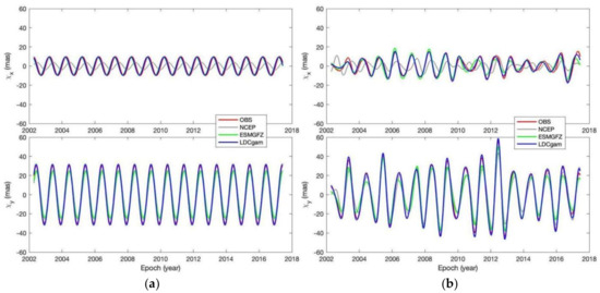
Figure 6.
Annual PM excitations. (a) Harmonic fitting according to Equation (2); (b) wavelet analyses based on the coif5 wavelet, as shown in Figure 4.
3.1.3. Semi-Annual Components
The semi-annual PM excitations are in fact higher harmonics of the annual ones, while, if a harmonic has a frequency that is an integer multiple of the fundamental frequency, it belongs to higher harmonics of the fundamental harmonic.
The semi-annual PM excitations for all four data sets obtained from both harmonic and wavelet analyses are displayed in Figure 7.
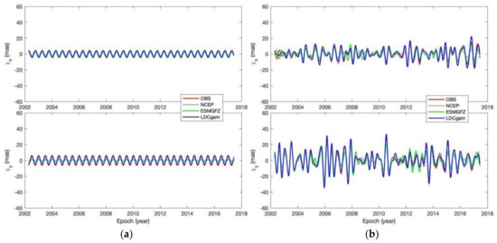
Figure 7.
Semi-annual PM excitations. (a) Harmonic fitting according to Equation (2); (b) wavelet analyses based on the coif5 wavelet, as shown in Figure 4.
3.2. Unexplained Excitations
If we view the PM excitations derived from the NCEP, ESMGFZ and LDCgam data sets as the explained parts, then their differences with respect to the observed excitation are the parts unexplained by these data sets with geophysical significance.
The unexplained excitations corresponding to the NCEP, ESMGFZ and LDCgam data sets are displayed in Figure 8, while their statistics are listed in Table 2.
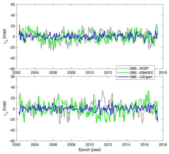
Figure 8.
The x- and y-components of unexplained polar motion excitations for the NCEP, ESMGFZ and LDCgam data sets, respectively.
Table 2.
Statistics of relevant time series (Unit: mas).
4. Discussion
From the harmonic and inharmonic quasi-biennial, annual and semi-annual components of PM excitations, as shown in Figure 5, Figure 6 and Figure 7, one can find that harmonic analysis tends to underestimate the amplitudes of fluctuations as its results represent the overall averages of the time series, while wavelet analysis can extract their changes in both amplitudes and periods. Therefore, the discrepancies between the observed PM excitation and modeled PM excitations, respectively from NCEP, ESMGFZ and LDCgam, are more evident in the results of wavelet analysis than in those of harmonic analysis, which is due to the fact that wavelet analysis is more suitable for analyzing nonstationary signals. The three components are further discussed below.
For the quasi-biennial components, Figure 5 shows that, in general, ESMGFZ and LDCgam can explain the observed quasi-biennial PM excitation better than NCEP does. In particular, Figure 5b illustrates notable changes in both amplitude and period for this component, which agrees with the nature of QBO [72]. In addition, wavelet analysis reveals that the x-component of QBO is relatively weak when the y-component is strong (for the period ~2006–2012), and vice versa (for the period ~2012–2016).
For the annual components, Figure 6 shows that, compared to the observed PM excitations, LDCgam agrees the best with the observation, while the NCEP data sets have notable phase discrepancies in the x-components, implying that the mass redistributions and relative motions are not well modeled around the meridian 0°E–180°E (more ocean, less land) compared to the 90°E–90°W (more land, less ocean) for the NCEP data sets. Moreover, while the amplitudes of these annual signals change markedly with time, the periods do not exhibit notable changes compared to the quasi-biennial one.
For the semi-annual components, Figure 7 shows that the phases are better modeled by all NCEP, ESMGFZ and LDCgam data sets than in the case of the annual components; however, the amplitudes determined by harmonic and wavelet analyses differ significantly from each other. The large discrepancy may indicate that the semi-annual component is highly nonstationary and thus highly non-harmonic, or substantial noises mix into this component when using wavelet analysis, which needs to be confirmed in further studies.
As for the unexplained components, both Figure 8 and Table 2 show that LDCgam has the best performance, mainly due to the following: (1) the LDCgam matter and motion terms are optimized by the LDC method; (2) the more advanced frequency-dependent PM excitation theory is used by the LDCgam data set, while the NCEP and ESMGFZ data sets adopt the traditional PM theory, which assumes that the Earth has a constant response to forcings with various frequencies (see Appendix B for more details).
5. Conclusions
This study aims to refine our understanding of the geophysical excitation of PM by applying harmonic and wavelet analyses to two GCM data sets and one combined solution, LDCgam. While GCM outputs are helpful to improve PM forecasts, we obtain the following findings.
- Mass redistributions and relative motions are not well modeled around the meridian 0°E–180°E (more ocean, less land) compared to the 90°E–90°W (more land, less ocean) for the NCEP data sets, especially at the annual frequency. Thus, further improvements are needed for the GCMs of NCEP data sets.
- Inclusion of monthly gravity data will lead to better geophysical excitations, such as the LDCgam. Thus, GCMs may need to adjust their parameters to minimize the differences between their outputs and monthly gravity data.
- The quasi-biennial and perhaps the semi-annual PM excitations are more nonstationary than annual ones, which implies that notable errors would be introduced if one applied harmonic analysis to them, and more advanced mathematical methods other than harmonic analysis are needed for better description of atmospheric, oceanic and hydrological dynamics.
- The LDCgam excitations, with Earth’s frequency-dependent responses considered, generally agree better with observed PM excitations than NCEP and ESMGFZ excitations, both using the traditional PM theory with the constant response assumption adopted. This might imply that consideration of the Earth’s frequency-dependent responses can improve our understanding of atmosphere–ocean–land water–solid Earth interactions, as the solid Earth is a complex body with both anelasticity and viscoelasticity.
These may be viewed as the highlights of this study.
Author Contributions
Conceptualization, H.L. and Y.Z.; methodology, Y.Z. and J.R.; software, Y.Z. and J.L.; validation, J.R.; formal analysis, H.L. and Y.Z.; investigation, H.L. and Y.Z.; resources, J.L.; data curation, H.L. and Y.Z.; writing—original draft preparation, H.L. and Y.Z.; writing—review and editing, J.R.; visualization, J.L.; supervision, J.R.; project administration, H.L. and Y.Z.; funding acquisition, H.L. and Y.Z. All authors have read and agreed to the published version of the manuscript.
Funding
This research was funded by the Hubei Provincial Natural Science Foundation of China, grant number 2021CFB515, and the National Natural Science Foundation of China, grant numbers 41874025 and 41474022. The APC was funded by the Natural Science Foundation of Hubei, grant number 2021CFB515.
Data Availability Statement
The ITRF2020 EOP is available at https://itrf.ign.fr/ftp/pub/itrf/itrf2020/ITRF2020_EOP-F1.DAT (accessed on 18 April 2022), and the NCEP, ECCO and ESMGFZ data are, respectively, available at http://files.aer.com/aerweb/AAM/, https://ecco-group.org/geodetic-variables.htm and http://rz-vm115.gfz-potsdam.de:8080/repository (accessed on 20 January 2022). The LDCmgm90 model and LDCgam data are, respectively, available at https://doi.org/10.6084/m9.figshare.7874384.v4 and https://doi.org/10.13140/RG.2.2.28698.49604 (accessed on 20 January 2022).
Acknowledgments
Wei Chen, at the School of Geodesy and Geomatics of Wuhan University, is highly appreciated for the insightful discussions and generous help in using the PM excitation theory with frequency-dependent responses of the Earth. We also thank the ITRF2020, NCEP/NCAR, ECCO and ESMGFZ teams, as well as Wei Chen, for making their data/models publicly available.
Conflicts of Interest
The authors declare no conflict of interest. The funders had no role in the design of the study; in the collection, analyses or interpretation of data; in the writing of the manuscript or in the decision to publish the results.
Appendix A
The Liouville equation for polar motion and the observed excitation are discussed below.
The linearized Liouville equation, derived from the conservation of angular momentum for a rotationally stratified Earth, is usually adopted to study polar motion excitations and can be written as [3,11,13,57,73]
where
is the complex Chandler frequency, p = x − iy are the coordinates of the CIP measured in the ITRS and χ = χ1 + iχ2 are the effective excitation functions (often called excitations for short).
Applying the Fourier Transformation (FT) to Equation (A1), one can obtain the excitation derived from polar motion observations via [32]
which is often called the geodetic (or observed) excitation. The geophysical excitations are usually compared with the observed excitation to quantify the contributions of certain geophysical processes to polar motion excitations.
Appendix B
The geophysical excitations of PM for Earth models with constant and frequency-dependent responses, respectively, are discussed below.
Given mass redistributions (evident as time-dependent products of inertia c(t)) and relative motions (evident as variable relative angular momenta h(t)) within the Earth system, another kind of excitation can also be derived by [3,8,57,74]
which is usually termed the geophysical excitation (here, Ω is the mean rotation rate of the Earth).
For an Earth model with the constant response assumption (namely, the Love numbers and thus PM transfer functions are constants), the traditional PM excitation theory gives TNL ≈ 1.61, TL ≈ 1.11 [3,11].
For an Earth model with frequency-dependent responses due to the effects of mantle anelasticity, quasi-fluid rheology, dynamic ocean tides and ocean pole tides, it is more suitable to evaluate the geophysical excitation in the frequency domain:
where the load and nonload polar motion transfer functions TL and TNL describe the responses of the stratified and deformable Earth and can be expressed as [57]
where the factor KD describes the elastic/anelastic (and possible loading) deformations; the factor KCMC describes core–mantle coupling/decoupling; the core–mantle coupling ratio η takes the value 1 for complete coupling and 0 for complete decoupling; δ equals 1 or 0, depending on whether the concerned terms load the Earth or not; k, k′ and ks are, respectively, the (degree 2 order 1) body-tide, load and secular Love numbers.
Using the consistent estimates of the fundamental Earth parameters in [57,75], A = 8.0085964 × 1037 kg m2, C = 8.0349010 × 1037 kg m2 and TL and TNL, respectively, take the values 1.141987 − 0.000056i and 1.660573 + 0.000044i for the weekly band, but 1.147018 + 0.000725i and 1.799738 + 0.009668i for the Chandler band. The imaginary parts of TL and TNL simply reflect the effects of mantle anelasticity and dissipative oceanic dynamics. More details about the frequency-dependent PM transfer functions can be found in Figure 7 and Table 6 of Chen et al. [57]. It is worth mentioning that relying on the 3-D displacement field measured by GPS and gravity variations from superconducting gravimeter records, Ding and Chao [58] determined the complex Love numbers at the Chandler band and provided an independent confirmation that the theory of the Earth’s frequency-dependent responses as presented by [57] is reliable.
Appendix C
The methods of deriving geophysical excitations from GCMs and LDCmgm90/GRACE/SLR data are discussed below.
By numerical integration of gridded data of the average temporal mass densities ρ and horizontal wind/current velocities (u, v) of the atmosphere, ocean and continental water from GCMs for the atmosphere, ocean and hydrology, the excitations for the matter and motion terms can be determined by [12,13,16,67]
and
For GRACE, SLR and LDCmgm90 degree-2 tesseral potential coefficients, mass redistributions c can be derived by [3,32]
as these potential coefficients reflect not only mass redistributions but also the associated loading deformations of the Earth (see [3] for a detailed discussion). In Equation (A10), M and a are, respectively, the mass and mean equatorial radius of the Earth.
Chen et al. [32,75] showed that the mean equatorial principal moment of inertia can be written as
where A20 = (4,841,694.6 ± 0.2) × 10−10 is the degree-2 zonal potential coefficient in the Earth’s principal axes system [75,76], and e = (C − A)/A is the dynamic ellipticity of the Earth.
Inserting Equations (A10) and (A11) into Equation (A8) and noting TL = (1 + k′) TNL, the matter-term excitation for GRACE or SLR can be written in a form related only to TNL and the potential coefficients [32]
where CS(f) is the Fourier Transformation of ΔC21(t) + iΔS21(t). One advantage of using Equation (A12) is that we can calculate the matter-term excitations directly from observed time-variable potential coefficients; another and more important advantage is that we can avoid using the Earth’s mass M or principal moment of inertia A, which still suffer from large uncertainties due to the poorly determined gravitational constant G [75,77].
References
- Petit, G.; Luzum, B. IERS Conventions (2010); IERS Technical Notes 36; Verlag des Bundesamts für Kartographie und Geodäsie: Frankfurt, Germany, 2010; ISBN 3-89888-989-6. [Google Scholar]
- Ratcliff, J.T.; Gross, R.S. Combinations of Earth Orientation Measurements: SPACE2008, COMB2008, and POLE2008; JPL Publ. 10-4; Jet Propulsion Laboratory: Pasadena, CA, USA, 2010; pp. 1–27.
- Gross, R.S. Earth rotation variations—Long period. In Treatise on Geophysics, 2nd ed.; Schubert, G., Ed.; Elsevier: New York, NY, USA, 2015; Volume 3, pp. 215–261. [Google Scholar]
- Ray, J. Precision and Accuracy of GNSS Positions; Lecture Presented at School of Geodesy and Geomatics; Wuhan University: Wuhan, China, 2015. [Google Scholar]
- Ray, J. Precision, accuracy, and consistency of GNSS products. In Encyclopedia of Geodesy; Grafarend, E.W., Ed.; Springer International: Cham, Switzerland, 2016. [Google Scholar] [CrossRef]
- Ray, J.; Rebischung, P.; Griffiths, J. IGS polar motion measurement accuracy. Geod. Geodyn. 2017, 8, 413–420. [Google Scholar] [CrossRef]
- Munk, W.H.; MacDonald, J.G.F. The Rotation of the Earth; Cambridge University Press: Cambridge, UK, 1960. [Google Scholar]
- Lambeck, K. The Earth’s Variable Rotation: Geophysical Causes and Consequences; Cambridge University Press: Cambridge, UK, 1980. [Google Scholar]
- Wahr, J.M. The effects of the atmosphere and oceans on the Earth’s wobble—I. Theory. Geophys. J. R. Astron. Soc. 1982, 70, 349–372. [Google Scholar] [CrossRef]
- Wahr, J.M. The effects of the atmosphere and oceans on the Earth’s wobble—II. Results. Geophys. J. R. Astron. Soc. 1983, 74, 451–487. [Google Scholar]
- Eubanks, T.M. Variations in the orientation of the Earth. In Contributions of Space Geodesy to Geodynamics: Earth Dynamics; Smith, D.E., Turcotte, D.L., Eds.; Geodynamics Series; American Geophysical Union: Washington, DC, USA, 1993; Volume 24, pp. 1–54. [Google Scholar]
- Gross, R.S.; Fukumori, I.; Menemenlis, D. Atmospheric and oceanic excitation of the Earth’s wobbles during 1980–2000. J. Geophys. Res. 2003, 108, 2370. [Google Scholar] [CrossRef]
- Barnes, R.T.H.; Hide, R.; White, A.A.; Wilson, C.A. Atmospheric angular momentum fluctuations, length-of-day changes and polar motion. Proc. R. Soc. Lond. Ser. A 1983, 387, 31–73. [Google Scholar] [CrossRef]
- Chao, B.F.; Au, A.Y. Atmospheric excitation of the Earth’s annual wobble: 1980–1988. J. Geophys. Res. 1991, 96, 6577–6582. [Google Scholar] [CrossRef]
- King, N.E.; Agnew, D.C. How large is the retrograde annual wobble? Geophys. Res. Lett. 1991, 18, 1735–1738. [Google Scholar] [CrossRef]
- Zhou, Y.H.; Salstein, D.A.; Chen, J.L. Revised atmospheric excitation function series related to Earth’s variable rotation under consideration of surface topography. J. Geophys. Res. 2006, 111, D12108. [Google Scholar] [CrossRef]
- Brzezinski, A.; Nastula, J.; Kolaczek, B.; Ponte, R.M. Oceanic excitation of polar motion from intraseasonal to decadal periods. In A Window on the Future of Geodesy; IAG, Symposia; Sanso, F., Ed.; Springer: Berlin/Heidelberg, Germany, 2005; Volume 128, pp. 591–596. [Google Scholar]
- Furuya, M.; Hamano, Y. Effect of the Pacific Ocean on the Earth’s seasonal wobble inferred from National Center for Environmental Prediction ocean analysis data. J. Geophys. Res. 1998, 103, 10131–10140. [Google Scholar] [CrossRef]
- Ponte, R.M.; Stammer, D.; Marshall, J. Oceanic signals in observed motions of the Earth’s pole of rotation. Nature 1998, 391, 476–479. [Google Scholar] [CrossRef]
- Ponte, R.M.; Stammer, D. Role of ocean currents and bottom pressure variability on seasonal polar motion. J. Geophys. Res. 1999, 104, 23393–23409. [Google Scholar] [CrossRef]
- Ponte, R.M.; Ali, A.H. Rapid ocean signals in polar motion and length of day. Geophys. Res. Lett. 2002, 29, 1711. [Google Scholar] [CrossRef]
- Johnson, T.J.; Wilson, C.R.; Chao, B.F. Oceanic angular momentum variability estimated from the Parallel Ocean Climate Model, 1988–1998. J. Geophys. Res. 1999, 104, 25183–25195. [Google Scholar] [CrossRef]
- Wunsch, J. Oceanic influence on the annual polar motion. J. Geodyn. 2000, 30, 389–399. [Google Scholar] [CrossRef]
- Chao, B.F.; O’Connor, W.P. Global surface-water-induced seasonal variations in the Earth’s rotation and gravitational field. Geophys. J. Int. 1988, 94, 263–270. [Google Scholar] [CrossRef]
- Kuehne, J.; Wilson, C.R. Terrestrial water storage and polar motion. J. Geophys. Res. 1991, 96, 4337–4345. [Google Scholar] [CrossRef]
- Wunsch, J. Oceanic and soil moisture contributions to seasonal polar motion. J. Geodyn. 2002, 33, 269–280. [Google Scholar] [CrossRef]
- Nastula, J.; Kolaczek, B. Analysis of hydrological excitation of polar motion. In Forcing of Polar Motion in the Chandler Frequency Band: A Contribution to Understanding Interannual Climate Change; Plag, H.P., Chao, B.F., Gross, R.S., van Dam, T., Eds.; Cahiers du Centre Européen de Géodynamique et de Séismologie: Luxembourg, 2005; Volume 24, pp. 149–154. [Google Scholar]
- Chen, J.L.; Wilson, C.R. Hydrological excitations of polar motion, 1993–2002. Geophys. J. Int. 2005, 160, 833–839. [Google Scholar] [CrossRef]
- Dobslaw, H.; Dill, R.; Grötzsch, A.; Brzezinski, A.; Thomas, M. Seasonal polar motion excitation from numerical models of atmosphere, ocean, and continental hydrosphere. J. Geophys. Res. 2010, 115, B10406. [Google Scholar] [CrossRef]
- Göttl, F.; Schmidt, M.; Seitz, F.; Bloßfeld, M. Separation of atmospheric, oceanic and hydrological polar motion excitation mechanisms based on a combination of geometric and gravimetric space observations. J. Geod. 2015, 89, 377–390. [Google Scholar] [CrossRef]
- Göttl, F.; Schmidt, M.; Seitz, F. Mass-related excitation of polar motion: An assessment of the new RL06 GRACE gravity field models. Earth Planets Space 2018, 70, 195. [Google Scholar] [CrossRef]
- Chen, W.; Li, J.C.; Ray, J.; Cheng, M.K. Improved geophysical excitations constrained by polar motion observations and GRACE/SLR time-dependent gravity. Geod. Geodyn. 2017, 8, 377–388. [Google Scholar] [CrossRef]
- Chen, W.; Luo, J.; Ray, J.; Yu, N.; Li, J.C. Multiple-data-based monthly geopotential model set LDCmgm90. Sci. Data 2019, 6, 228. [Google Scholar] [CrossRef] [PubMed]
- Liu, L.; Hsu, H.; Grafarend, E.W. Normal Morlet wavelet transform and its application to the Earth’s polar motion. J. Geophys. Res. 2007, 112, B08401. [Google Scholar] [CrossRef]
- Chao, B.F.; Chung, W.; Shih, Z.; Hsieh, Y. Earth’s rotation variations: A wavelet analysis. Terra Nova 2014, 26, 260–264. [Google Scholar] [CrossRef]
- Luo, J.; Chen, W.; Ray, J.; Li, J.C. Excitations of length-of-day seasonal variations: Analyses of harmonic and inharmonic fluctuations. Geod. Geodyn. 2020, 11, 64–71. [Google Scholar] [CrossRef]
- Cheng, M.K.; Tapley, B.D. Variations in the Earth’s oblateness during the past 28 years. J. Geophys. Res. 2004, 109, B09402. [Google Scholar] [CrossRef]
- Cheng, M.K.; Tapley, B.D.; Ries, J.C. Deceleration in the Earth’s oblateness. J. Geophys. Res. Solid Earth 2013, 118, 740–747. [Google Scholar] [CrossRef]
- Loomis, B.D.; Rachlin, K.E.; Luthcke, S.B. Improved Earth oblateness rate reveals increased ice sheet losses and mass-driven sea level rise. Geophys. Res. Lett. 2019, 46, 6910–6917. [Google Scholar] [CrossRef]
- Cheng, M.K.; Ries, J.C.; Tapley, B.D. Variations of the Earth’s figure axis from satellite laser ranging and GRACE. J. Geophys. Res. 2011, 116, B01409. [Google Scholar] [CrossRef]
- Loomis, B.D.; Rachlin, K.E.; Wiese, D.N.; Landerer, F.W.; Luthcke, S.B. Replacing GRACE/GRACE-FO C30 with satellite laser ranging: Impacts on Antarctic Ice Sheet mass change. Geophys. Res. Lett. 2020, 47, e2019GL085488. [Google Scholar] [CrossRef]
- Taplay, B.D.; Bettadpur, S.; Ries, J.C.; Thompson, P.F.; Watkins, M.M. GRACE measurements of mass variability in the Earth system. Science 2004, 305, 503–505. [Google Scholar] [CrossRef] [PubMed]
- Bettadpur, S. UTCSR Level-2 Processing Standards Document for Level-2 Product Release 0006; Report No. GRACE 327–742; Center for Space Research: Austin, TX, USA, 2018. [Google Scholar]
- Dahle, C.; Flechtner, F.; Murböck, M.; Michalak, G.; Neumayer, H.; Abrykosov, O.; Reinhold, A.; König, R. GFZ Level-2 Processing Standards Document for Level-2 Product Release 0006; Report No. STR18/04-data; Deutsches Geo Forschungs Zentrum: Potsdam, Germany, 2018. [Google Scholar]
- Yuan, D. JPL Level-2 Processing Standards Document for Level-2 Product Release 06; Report No. GRACE 327–744; Jet Propulsion Laboratory: Pasadena, CA, USA, 2018.
- Mayer-Gürr, T.; Behzadpour, S.; Kvas, A.; Ellmer, M.; Klinger, B.; Strasser, S.; Zehentner, N. ITSG-Grace 2018-Monthly, Daily and Static Gravity Field Solutions from GRACE. Available online: https://dataservices.gfz-potsdam.de/icgem/showshort.php?id=escidoc:3600910 (accessed on 20 January 2022).
- Watkins, M.M.; Wiese, D.N.; Yuan, D.N.; Boening, C.; Landerer, F.W. Improved methods for observing Earth’s time variable mass distribution with GRACE using spherical cap mascons. J. Geophys. Res. Solid Earth 2015, 120, 2648–2671. [Google Scholar] [CrossRef]
- Wiese, D.N.; Landerer, F.W.; Watkins, M.M. Quantifying and reducing leakage errors in the JPL RL05M GRACE mascon solution. Water Resour. Res. 2016, 52, 7490–7502. [Google Scholar] [CrossRef]
- Save, H.; Bettadpur, S.; Tapley, B.D. High resolution CSR GRACE RL05 mascons. J. Geophys. Res. Solid Earth 2016, 121, 7547–7569. [Google Scholar] [CrossRef]
- Brzeziński, A.; Nastula, J.; Kołaczek, B. Seasonal excitation of polar motion estimated from recent geophysical models and observations. J. Geodyn. 2009, 48, 235–240. [Google Scholar] [CrossRef]
- Swenson, S.; Wahr, J. Post-processing removal of correlated errors in GRACE data. Geophys. Res. Lett. 2006, 33, L08402. [Google Scholar] [CrossRef]
- Kusche, J. Approximate decorrelation and non-isotropic smoothing of time-variable GRACE-type gravity field models. J. Geod. 2007, 81, 733–749. [Google Scholar] [CrossRef]
- Guo, J.Y.; Duan, X.J.; Shum, C.K. Non-isotropic Gaussian smoothing and leakage reduction for determining mass changes over land and ocean using GRACE data. Geophys. J. Int. 2010, 181, 290–302. [Google Scholar] [CrossRef]
- Chen, W.; Ray, J.; Shen, W.B.; Huang, C.L. Polar motion excitations for an Earth model with frequency-dependent responses:2 Numerical tests of the meteorological excitations. J. Geophys. Res. Solid Earth 2013, 118, 4995–5007. [Google Scholar] [CrossRef]
- Göttl, F.; Groh, A.; Schmidt, M.; Schröder, L.; Seitz, F. The influence of Antarctic ice loss on polar motion: An assessment based on GRACE and multi-mission satellite altimetry. Earth Planets Space 2021, 73, 99. [Google Scholar] [CrossRef]
- Luo, J.; Chen, W.; Ray, J.; van Dam, T.; Li, J.C. A Loading Correction Model for GPS Measurements Derived from Multiple-Data Combined Monthly Gravity. Remote Sens. 2021, 13, 4408. [Google Scholar] [CrossRef]
- Chen, W.; Ray, J.; Li, J.C.; Huang, C.L.; Shen, W. Polar motion excitations for an Earth model with frequency-dependent responses: 1. A refined theory with insight into the Earth’s rheology and core-mantle coupling. J. Geophys. Res. Solid Earth 2013, 118, 4975–4994. [Google Scholar] [CrossRef]
- Ding, H.; Chao, B.F. Solid pole tide in global GPS and superconducting gravimeter observations: Signal retrieval and inference for mantle anelasticity. Earth Plan. Sci. Lett. 2017, 459, 244–251. [Google Scholar] [CrossRef]
- Altamimi, Z. The ITRF2020 Solutions for Earth Orientation Parameters. Available online: https://itrf.ign.fr/ftp/pub/itrf/itrf2020/ITRF2020_EOP-F1.DAT (accessed on 24 April 2022).
- Bourke, W. A multi-level spectral model. I. Formulation and hemispheric integrations. Mon. Wea. Rev. 1974, 102, 687–701. [Google Scholar] [CrossRef]
- Machenhauer, B.; Rasmussen, E. On the Integration of the Spectral Hydrodynamical Equations by a Transform Method; Report No. 3; Institute for Theoretical Meteorology, University of Copenhagen: Copenhagen, Denmark, 1972. [Google Scholar]
- Gross, R.S. An improved empirical model for the effect of long period ocean tides on polar motion. J. Geod. 2009, 83, 635–644. [Google Scholar] [CrossRef]
- Owens, R.G.; Hewson, T.D. ECMWF Forecast User Guide. 2018. Available online: https://confluence.ecmwf.int/display/FUG/Forecast+User+Guide (accessed on 12 January 2022).
- Jungclaus, J.H.; Fischer, N.; Haak, H.; Lohmann, K.; Marotzke, J.; Matei, D.; Mikolajewicz, U.; Notz, D.; von Storch, J.S. Characteristics of the ocean simulations in the Max Planck Institute Ocean Model (MPIOM) the ocean component of the MPI-Earth system model. J. Adv. Model Earth Syst. 2013, 5, 422–446. [Google Scholar] [CrossRef]
- Dill, R. Hydrological Model LSDM for Operational Earth Rotation and Gravity Field Variations; Scientific Technical Report STR08/09; Deutsches Geo Forschungs Zentrum: Potsdam, Germany, 2008. [Google Scholar]
- Dill, R.; Dobslaw, H. Numerical simulations of global-scale high-resolution hydrological crustal deformations. J. Geophys. Res. Solid Earth 2013, 118, 5008–5017. [Google Scholar] [CrossRef]
- Salstein, D.A.; Kann, D.M.; Miller, A.J.; Rosen, R.D. The subbureau for atmospheric angular momentum of the International Earth Rotation Service (IERS): A meteorological data center with geodetic applications. Bull. Am. Meteorol. Soc. 1993, 74, 67–80. [Google Scholar] [CrossRef][Green Version]
- Wunsch, C.; Stammer, D. Atmospheric loading and the oceanic “inverted barometer” effect. Rev. Geophys. 1997, 35, 79–107. [Google Scholar] [CrossRef]
- Dobslaw, H.; Bergmann-Wolf, I.; Dill, R.; Forootan, E.; Klemann, V.; Kusche, J.; Sasgen, I. The updated ESA Earth System Model for future gravity mission simulation studies. J. Geod. 2015, 89, 505–513. [Google Scholar] [CrossRef]
- Dobslaw, H.; Bergmann-Wolf, I.; Dill, R.; Poropat, L.; Thomas, M.; Dahle, C.; Esselborn, S.; König, R.; Flechtne, F. A new high-resolution model of non-tidal atmosphere and ocean mass variability for de-aliasing of satellite gravity observations: AOD1B RL06. Geophys. J. Int. 2017, 211, 263–269. [Google Scholar] [CrossRef]
- Daubechies, I. Ten Lectures on Wavelets; Cambridge University Press: Cambridge, UK, 1992. [Google Scholar]
- Baldwin, M.P.; Gray, L.J.; Dunkerton, T.J.; Hamilton, K.; Haynes, P.H.; Randel, W.J.; Holton, J.R.; Alexander, M.J.; Hirota, I.; Horinouchi, T.; et al. The quasi-biennial oscillation. Rev. Geophys. 2001, 39, 179–229. [Google Scholar] [CrossRef]
- Brzeziński, A.; Capitaine, N. The use of the precise observations of the celestial ephemeris pole in the analysis of geophysical excitation of earth rotation. J. Geophys. Res. 1993, 98, 6667–6675. [Google Scholar] [CrossRef]
- Dickman, S.R. Evaluation of “effective angular momentum function” formulations with respect to core-mantle coupling. J. Geophys. Res. 2003, 108, 2150. [Google Scholar] [CrossRef]
- Chen, W.; Li, J.C.; Ray, J.; Shen, W.B.; Huang, C.L. Consistent estimates of the dynamical figure parameters of the Earth. J. Geod. 2015, 89, 179–188. [Google Scholar] [CrossRef]
- Heiskanen, W.A.; Moritz, H. Physical Geodesy; W.H. Freeman: San Francisco, CA, USA, 1967. [Google Scholar]
- Groten, E. Fundamental parameters and current (2004) best estimates of the parameters of common relevance to astronomy, geodesy, and geodynamic. J. Geod. 2004, 77, 724–797. [Google Scholar] [CrossRef]
Publisher’s Note: MDPI stays neutral with regard to jurisdictional claims in published maps and institutional affiliations. |
© 2022 by the authors. Licensee MDPI, Basel, Switzerland. This article is an open access article distributed under the terms and conditions of the Creative Commons Attribution (CC BY) license (https://creativecommons.org/licenses/by/4.0/).