Abstract
Seagrass meadows are one of the blue carbon ecosystems that continue to decline worldwide. Frequent mapping is essential to monitor seagrass meadows for understanding change processes including seasonal variations and influences of meteorological and oceanic events such as typhoons and cyclones. Such mapping approaches may also enhance seagrass blue carbon strategy and management practices. Although unmanned aerial vehicle (UAV) aerial photography has been widely conducted for this purpose, there have been challenges in mapping accuracy, efficiency, and applicability to subtidal water meadows. In this study, a novel method was developed for mapping subtidal and intertidal seagrass meadows to overcome such challenges. Ground truth seagrass orthophotos in four seasons were created from the Futtsu tidal flat of Tokyo Bay, Japan, using vertical and oblique UAV photography. The feature pyramid network (FPN) was first applied for automated seagrass classification by adjusting the spatial resolution and normalization parameters and by considering the combinations of seasonal input data sets. The FPN classification results ensured high performance with the validation metrics of 0.957 overall accuracy (OA), 0.895 precision, 0.942 recall, 0.918 F1-score, and 0.848 IoU, which outperformed the conventional U-Net results. The FPN classification results highlighted seasonal variations in seagrass meadows, exhibiting an extension from winter to summer and demonstrating a decline from summer to autumn. Recovery of the meadows was also detected after the occurrence of Typhoon No. 19 in October 2019, a phenomenon which mainly happened before summer 2020.
1. Introduction
Coastal blue carbon ecosystems, such as mangroves, salt marshes, and seagrass meadows, play a crucial role in supplying environmental functions such as providing shelter for fisheries, performing water purification, enhancing soil stability, decreasing coastal erosion, supplementing nutrients, protecting coastlines [1], and mitigating climate change by sequestering carbon from the atmosphere [2]. They are regarded as the most efficient ecosystem for carbon storage but are also the most rapidly disappearing ecosystem worldwide. Among them, seagrass meadows serve as habitats in subtidal and intertidal zones and continue to decline due to the fact of environmental [3] and climate change [4]; episodic events, including heatwaves [5], storms [6], and tsunamis [7]; anthropogenic activities [8]. Monitoring of seagrass meadows is essential for understanding the mechanism of their changes and promoting the social implementation of its blue carbon policy [9].
Extensive efforts to monitor seagrass meadows have been engaged through in situ surveys, including diving surveys [10] and sampling-based surveys [11], which are accurate but laborious, costly, and time-consuming. Passive remote sensing (Quickbird-2 [12], IKONOS [13], Landsat 5, and Landsat 7 [14]) and active remote sensing (side-scan sonar [15] and airborne Lidar [16]) have also been widely used to monitor seagrass meadows; however, obtainment of frequent and high-resolution images that will contribute toward understanding the processes of changes in seagrass meadows and will aid in the promotion of blue carbon management may be costly; moreover, the thick cloud affects the timely acquisition of satellite image resources. Recently, unmanned aerial vehicles (UAVs), also known as drones, have attracted attention for application in coastal ecosystem mapping [17]. Although unmanned aerial vehicles are restricted by the maximum distance and flight time as well as policy restrictions in different regions, they can be used to acquire high-quality orthophoto images in small areas with high resolution and high frequency owing to their flexibility including avoiding the influence of cloud cover [18].
Collection and classification of seagrass images obtained using drones remain challenging. Duffy et al. [19] compared unsupervised and object-based image analysis (OBIA) classification methods adopted for acquiring intertidal seagrass orthophotos. Although these traditional machine learning methods yield high-accuracy, generalization ability limitations lead to the achievement of unsatisfactory results when a trained model is applied to a new data set [20]. Deep learning methods have gained popularity for coping with the generalization problem owing to their advantages in digging semantic values after convolution. For example, Yamakita et al. [21] confirmed that a deep convolutional generative adversarial network showed better results than the fully convolutional network for classifying different objects, including seagrass, by using aerial and satellite images (QuickBird). However, the deep convolutional generative adversarial network may exhibit limitations, such as collapsing generators, and is highly sensitive to hyper-parameter selections [22]. Moniruzzaman et al. [23] demonstrated that a faster region-based convolutional neural network yielded good results for classifying underwater video images of seagrass. However, the approach of the faster region-based convolutional neural network depends on a very time-consuming algorithm for object location assumption [24]. Recently, U-Net has been applied for drone image classification because it requires fewer images and has a simple stable structure. Hobley et al. [25] and Jeon et al. [26] applied U-Net to classify intertidal seagrass orthophotos. Although their results were accurate for intertidal waters, their applicability to subtidal water seagrass meadows posed challenges. U-Net is also unsuitable for classifying small seagrass objects in the image [27]. The feature pyramid network (FPN) was first introduced for object detection. It consists of a top-down pathway that can be used to generate different resolution layers, and classification in these layers helps classify small objects in the image. [28]. As studies have not been reported on the application of FPN to classify seagrass images, this study aimed to evaluate its performance compared with that of U-Net.
Preprocessing images, such as resolution adjustment, the normalization process, and a combination of input data sets, is essential for increasing classification accuracy [29,30], especially for submerged seagrass images with sun glint and scattering due to the presence of waves. The noise induced by sun glint and scattering due to the fact of waves in the original drone photos might lead to the information loss of submerged target objects. Noises in images (i.e., glint, contrast, and compression) negatively affect the model learning of the features of images [31]. Image normalization can help alleviate the brightness difference attributable to changes in lighting conditions during a long-time mapping mission [32]. Color calibration aids the unification of the features of images before the mosaic of the images [33]; however, it may not be adequate to perform corrections for brightness difference in subtidal and intertidal seagrass images. Hence, further image normalization after mosaic is necessary, such as by using Gaussian blur [34], which is a widely applied smoothing technology based on the Gaussian function. Depending on the number of classification classes and the amount of data in each class of input training data, the combination of different input data sets yields different classification accuracies [35]. To our knowledge, existing studies have not reported the assessment of the effect of such aspects on the classification of subtidal and intertidal seagrass images, which we aimed to discuss in the present study.
The Futtsu tidal flat in Tokyo Bay, Japan, has been regarded as a study site for monitoring seagrass meadows [36]. However, few studies have reported the identification of seasonal variations and the influence of meteorological and oceanic events, including typhoon impacts, using drone images. Typhoon Hagibis, one of the biggest typhoons documented since 1977 in Japan [37], hit Tokyo Bay in October 2019; however, there was no occurrence of a typhoon in Tokyo Bay in 2020. Therefore, during 2020, the Futtsu tidal flat was a suitable study site for examining seagrass recovery after the occurrence of typhoons.
The objective of the present study was to develop a novel automated method for mapping subtidal and intertidal seagrass meadows with high accuracy by applying FPN to drone orthophotos. First, we generated ground truth polygons of subtidal and intertidal seagrass meadows. Thereafter, we formulated an FPN application protocol for mapping and evaluated its performance compared to that of U-Net-based classification. An investigation on the influence of resolution, normalization, and a combination of data sets was also performed to enhance classification accuracy. Finally, seasonal variations in seagrass meadows were identified, and the influence of typhoons was assessed.
2. Materials and Methods
The present study comprised image collection, image classification, and variation identification (see Figure 1).
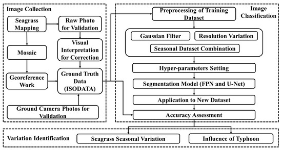
Figure 1.
Workflow of seagrass classification and area evaluation.
2.1. Study Site
The Futtsu tidal flat is located in the middle of Tokyo Bay in Futtsu City, Chiba Prefecture, Japan (Figure 2), and presents with the largest seagrass meadows in the bay. Three seagrass species, namely, Zostera marina (eelgrass), Zostera caulescens, and Zostera japonica (Japanese eelgrass), inhabit the meadows with eelgrass as the dominant species. The study area was approximately 1.8 × 0.7 km with a water depth of 0–3 m [38] as shown in Figure 2C.
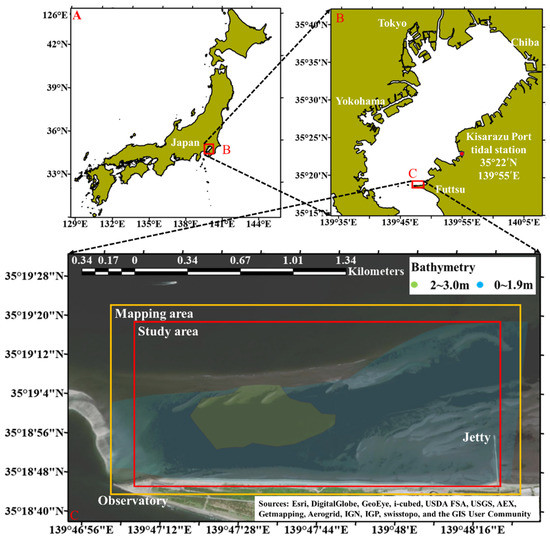
Figure 2.
Location of the Futtsu tidal flat in Tokyo Bay. The study area (red box) extended from the observatory in the west to the jetty in the east, and the mapping area (yellow box) was slightly larger than the study area. Other areas are restricted by policy. The bathymetry is also shown here [38,39].
2.2. Seagrass Image Collection
We acquired aerial photos of seagrass meadows from January 2020 to March 2021 using a DJI Phantom 4 Pro drone. The seagrass was submerged underwater when the images were collected. Vertical photos were acquired under conditions of cloudy, calm wind speeds lower than 2 m/s and low tide conditions to obtain a clear image of subtidal and intertidal seagrass meadows [40]. Oblique photos were occasionally obtained in the case of a low solar zenith angle (less than 50°) in sunny weather to avoid sun glint and scattering due to the presence of waves [41,42] as shown in Figure 3. Detailed mapping information is presented in Table 1. Notably, the generated orthophotos for each season were based on photos collected on one or separate dates at the same water level; additional images were collected during the same season to compensate for the missing details of the orthophotos. Drone images in the spring of 2020 could not be collected due to the outbreak of COVID-19; thus, these images were collected in 2021.
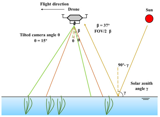
Figure 3.
Schematic diagram of oblique photography. Half of the field of view (FOV/2) β, solar zenith angle γ, and tilted camera degree θ should satisfy: 90° − γ > β − θ [43]. The flight direction and tilted camera degree should be adjusted according to the sun direction to minimize the FOV/2. The tilted camera angle θ was 15°, and the FOV/2 β was calculated to be 37° [44]. The solar zenith angle γ was approximately 45° when mapping, avoiding sun glint.

Table 1.
Photography specifications for seagrass meadows. Tidal level data at Kisarazu Port (Figure 2B) were obtained from the Japan Meteorological Agency [45].
2.3. Generation of Ground Truth Data
It is essential to establish accurate ground truth data as a training data set for deep learning. Nine ground control points (GCPs) were evenly set on semi-permanent marks, and post-processed kinematic (PPK) was applied to obtain the accurate coordinates of the GCPs (see Figure 4). Original photos were processed through the structure from motion (SfM) using the photo mosaic software Metashape (Agisoft) [46] to generate orthophotos. The same season additional photos replaced the photos with missing details when generating the orthophotos. Many additional tie points were considered to aid relative georeferencing based on the spectral signature difference after the GCPs’ georeferencing [47].
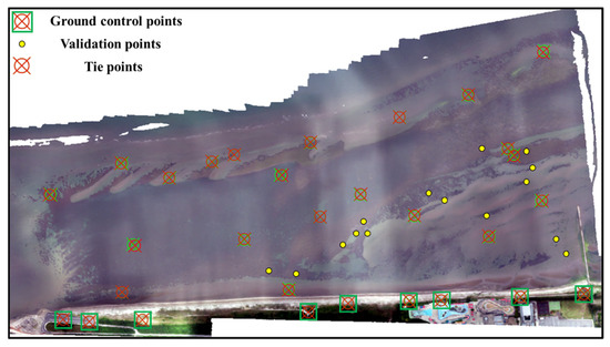
Figure 4.
Locations of ground control and validation points. Additional tie points were added to conduct the relative georeferencing work. The primary validation of the classification results was based on the raw photos obtained from the drone with clear information.
We used the iterative self-organizing data analysis technique algorithm (ISODATA) to classify seagrass meadows [48] and conducted visual interpretation to correct the classification results, creating ground truth data for deep learning models. The entire orthophoto was split into five parts, each of which was processed independently to enhance processing speed (Figure 5 is presented to demonstrate the processing of part 4). Each part was first resampled to a 0.5 m resolution to eliminate image noise, followed by pre-classification into 40 categories after conducting unsupervised classification in a class size of 20 and a sampling interval of 10 (one cell out of every ten blocks of cells was used in the cluster calculation). According to the major color difference in the original photos (seagrass meadows are indicated in green, and sediments are indicated in white), 40 pre-classified categories were reclassified into seagrass and non-seagrass categories. As reclassification results varied in different places in part 4, we further clipped the reclassification results and separated them into newly created three layers in the contents table of ArcGIS. In layer 1 (Figure 5C–E), the majority filter was applied to improve the results by eliminating the remaining noise, and visual interpretation was conducted to correct the detrital manually. Following the same process, layer 2 (Figure 5F,G) and layer 3 (Figure 5H,I) were classified, and the three layers were merged to obtain the final classification results (Figure 5J). By connecting the results of all five parts to obtain single ground truth data, ground truth polygons and binary rasters for seagrass meadows were created. Following the procedures, seasonal orthophotos with ground truth polygons and binary rasters were generated.
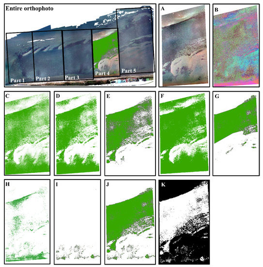
Figure 5.
The creation process of ground truth data. Part 4 is used for demonstrating the process: (A) clipped resample orthophoto; (B) results after performing ISODATA; (C) layer 1: pre-classified into two categories (seagrass and non-seagrass); (D) layer 1: results after the majority filter; (E) layer 1: results after manual correction; (F) layer 2: repeated for pre-classification into two categories; (G) layer 2: results after the majority filter and manual correction; (H) layer 3: repeated for pre-classification into two categories; (I) layer 3: results after the majority filter and manual correction; (J) merge classification results of E, G, and I (layers 1–3); (K) binary ground truth data.
The results were validated based on color and texture information of seagrass and non-seagrass from the high-resolution raw photos obtained by the drone. In addition, proximate photos of seagrass at 15 stations with location information were recorded in places accessible by foot using a waterproof camera with GPS (Nikon COOLPIX W300) on 17 July and 23 April 2019 (see Figure 4). These camera photos were addressed on the created ground truth data results for further validation.
2.4. Seagrass Classification
2.4.1. Segmentation Model
FPN was applied in the preprocessing and classification for the new data set of winter of 2020. FPN comprised bottom-up and top-down pathways as shown in Figure 6 [49]. The bottom-up pathway in the left is the normal network of convolution used to extract the features of the original image with a 2 step scaling. As the bottom-up process continues, the spatial resolution decreases, while the semantic value increases. As the low semantic value and the high quality of the original photo reduce the speed of calculation, the original high-quality image in the bottom layer was not used for semantic detection. FPN contains another top-down pathway to compensate for the problem by generating high-quality layers from the high semantic value layer. Although the regenerated layers presented with high semantic values, the locations of the objects were not accurate. Thus, the top-down pathway was combined with the same spatial size features from the bottom-up process. As shown in the red, solid line box in Figure 6, the upsampling approach was considered using nearest neighbor methods to change the spatial resolution twice, and a 1 × 1 convolution layer was used to reduce the dimensions of the feature channel when the feature maps in the two pathways were merged with element-wise addition. Thereafter, the feature maps generated contained high-accuracy location information and high-quality semantic features, which can help predict objects of different sizes in different layers by considering the advantage of different resolution images and the semantic values of object features in the original image. These multi-scale object detection and segmentation characteristics were the main differences from those of U-Net. When deciding which layer the region of interest should be assigned, the following equation was used [49]:
where is 4, and are the width and height of the region of interest, respectively, and the whole calculation result is rounded down to obtain the , which means that layer k in the FPN is used to generate the feature patch. The particular structure of an FPN helps identify the location of small objects in the image, which renders feasibility and convenience to FPN training [50].
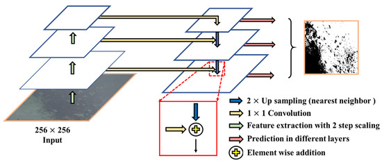
Figure 6.
The feature pyramid network (FPN) framework included two independent parts: the original image was imported from the left bottom-up structure, and predictions were performed at every layer of the right top-down paths [49].
U-Net was used to classify the same data set with similar preprocessing procedures as FPN. U-Net consists of an encoder and decoder [51] (see Figure 7), which helps save the essential features by reducing the dimensionality of the inputted orthophoto images in the left part of the model and consists of five blocks for feature extraction (two 3 × 3 convolutions) and downsampling (2 × 2 max-pooling after convolutions), wherein the base number of kernels is determined in the first block. When feature extraction is finished in the last block, the decoder acts in the opposite direction by increasing the dimensionality and by transforming the high convolutional information into the original spatial information. The decoder contains four blocks, each with 2 × 2 up-convolutions and 3 × 3 convolutions. These two parts are then concatenated with the same feature map size; thus, the number of feature channels is doubled, and low-level information is included to obtain deep features. The model is suitable for classifying objects that are close to each other by using the following loss function [51]:
where is the loss function of softmax, is the true label of each pixel, and is a weight map that assigns more weight to points near the boundary. The prediction is commenced after the decoder process ends in the last block; this is regarded as the end-to-end segmentation process of the original images [52]. Unlike FPN, U-Net only makes predictions in the last layer.
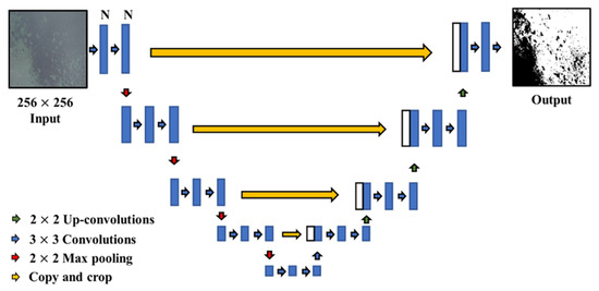
Figure 7.
The framework of U-Net. Images are imported into the encoder for convolution and max-pooling and are then processed with copy and crop, up-convolution, and convolutions in the decoder to finish classification [51].
2.4.2. Input Data Preparation
The orthophotos and ground truth binary rasters were processed with a random sliding window into small images and corresponding binary rasters. The number of cropped images was the same throughout all seasonal data sets, and few images were presented with overlapping. Input data sets for the training process were generated as a combination of the training data set (80%), testing data set (10%), and validation data set (10% for self-validation). The original images (resolution: 0.05 m) were resampled to 0.1, 0.2, 0.5, 1, 2, and 4 m to assess the influence of spatial resolution on the accuracy of seagrass classification. The model was trained at each resolution, and the optimal resolution was selected in terms of the overall accuracy (OA, see Equation (3)) for the subsequent preprocessing step. These protocols were implemented for the subsequent preparation of the input data sets.
The application of Gaussian blur is expected to enhance classification accuracy. The optimal Gaussian blur pixel radius was determined in terms of OA by conducting a series of experiments with different pixel radii of 1001, 901, 801, 701, 601, 501, and 401 (unit: pixel) along with a group without Gaussian blur application to orthophotos with the selected resolution.
We designed a series of experiments to examine the influence of combinations of input data sets on the model’s generalized classification accuracy and implementation efficiency. A total of 15 combinations () were obtained for the four seasonal data sets (see No.1–4 in Table 1).
2.4.3. Hyper-Parameter Tuning
We adopted a set of default hyper-parameters provided in pre-experiment for the FPN, as FPN problems are primarily attributed to the input data set rather than hyper-parameter tuning [28], which was computationally extremely costly in the FPN. Hyper-parameter tuning of U-Net was conducted in terms of three hyper-parameters of the batch size, base number of kernels, and learning rate using the prepared input data set. Previous studies have suggested that an orthogonal experimental design may help save computational resources by reducing experimental cases [53]. By adopting such a design (Table 2), the number of experiments (27; three factors each with three levels, 33 = 27) was reduced to nine, and such experiments were conducted in U-Net tuning.
Table 2.
Orthogonal experimental design for hyper-parameter tuning in U-Net.
2.5. Accuracy Assessment
OA is the criterion for selecting the input data set preparation and hyper-parameter tuning [54]. The classification results of the final trained models were converted to a confusion matrix, wherein each pixel in the images was classified into one of the four principal terms of true positive (TP), false positive (FP), false negative (FN), and true negative (TN), compared with the ground truth data. For evaluation, the following five criteria were selected: OA, precision, recall, F1-score, and intersection over union (IoU), defined by the following:
where their value range was between 0 and 1 [55].
3. Results
3.1. Verification of the Ground Truth Data
Five ground truth data in four seasons were established as shown in Figure 8. Seagrass meadows were distributed inside green polygons. Figure 9 demonstrates the verification of the ground truth data using high-resolution raw images obtained using drone photos and camera photos. The created seagrass polygons were consistent with the boundary lines between the seagrass and non-seagrass beds.
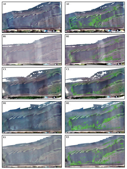
Figure 8.
Orthophoto images and corresponding ground truth for winter (A1,A2), summer (B1,B2), and autumn (C1,C2) in 2020 and images for winter (D1,D2) and spring (E1,E2) in 2021. The green polygon lines in the right images show the boundaries between seagrass and non-seagrass; seagrass was distributed inside the green polygon.
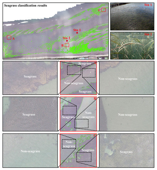
Figure 9.
Verification of seagrass ground truth data. Summer data were used for illustration; depicted above is the seagrass polygon on summer orthophoto; (A–C) and the corresponding original raw photos for seagrass and non-seagrass validated the ground truth data; Stn. 1 and Stn. 2 are the sampling sites from camera photos.
3.2. Seagrass Mapping Results
3.2.1. Selection Results of the Input Data Set
The influences of preprocessing levels in terms of image resolution and normalization using Gaussian blur on the FPN classification are summarized by OA in Table 3. The OA value increased with a decrease in the resolution from 0.05 to 2 m and then decreased, with the highest OA value of 0.971 achieved at a 2 m resolution, a finding which is consistent with the previous cognition for drone image classifications [56]. The highest OA value of 0.976 was achieved with a Gaussian blur radius of 901.
Table 3.
Selection results for the input data set of resolution and normalization preprocess.
By selecting a spatial resolution of 2 m and Gaussian blur radius of 901, 15 experiments (see Section 2.4.2) were conducted, and their results are summarized in Table 4. In principle, the self-validation results (from the 10% validation data set), which represented the accurate classification ability, increased as the class number decreased, while the cross-validation results in each season, which represented the generalization ability, decreased as the class number decreased. The mean OA value in the last column, which represents the average of the self-validation and cross-validation results, revealed a balance between accuracy and generalization ability. The mean OA also decreased with a decrease in the class number of the data set. The optimum result was obtained in No. 1 using four seasons data set in terms of OA (a mean value of 0.965) and applicability to any season, and this would be the best combination, despite not being cost-effective. Number 15 showed relatively high accuracy and generalization ability for using only one data set in the winter, and this may be deemed an easy and inexpensive option.
Table 4.
Experimental results of the input data set adjustment.
The same experiments were conducted for U-Net, revealing that the experiment using four seasons data set with a spatial resolution of 2 m and Gaussian blur radius of 701 showed the best mean OA of 0.956.
3.2.2. Hyper-Parameter Tuning for U-Net
The hyper-parameters of the FPN were set to default values as described in Section 2.4.3. Tuning results for the hyper-parameters of U-Net demonstrated that T04 was the best combination, as shown in Table 5, which was adopted in further applications.
Table 5.
Orthogonal experimental results for the hyper-parameter tuning of U-Net.
3.2.3. Model Testing via Application to a New Data Set
For testing, the FPN and U-Net models were applied to classify seagrass meadows for a new data set in winter 2021 (see Table 1), which was not used for model development. We trained the models with four seasons input data set in 2 m resolution processed with Gaussian blur in 901 radius (701 radius for U-Net). The results are presented in Table 6 and Figure 10. To verify the importance of every step of the preprocessing procedure, FPN and U-Net models in every stage of the preprocessing were applied to the new data set. The FPN model with original and adjusted resolutions yielded unsatisfactory results (Figure 10A,B). When a suitable Gaussian blur was applied to the data set, the FPN classification achieved the highest accuracy (Figure 10C). The U-Net model with the original and proper spatial resolution also yielded unsatisfactory results (Figure 10D,E); their accuracy was not significantly different from the FPN model’s results using the same data set process procedures. When further preprocessed with Gaussian blur, the model performance worsened (Figure 10F). When only the spatial resolution orthophoto was adjusted, we obtained the highest classification results.
Table 6.
Classification results for the new data set in winter 2021 obtained from different models.
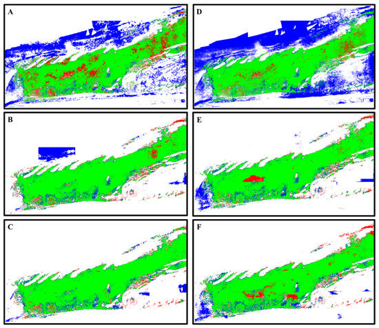
Figure 10.
Classification results in winter 2021: green, TP; blue, FP; red, FN; white, TN. (A) FPN (original resolution); (B) FPN (adjusted resolution); (C) FPN (adjusted resolution and Gaussian blur); (D) U-Net (original resolution); (E) U-Net (adjusted resolution); (F) U-Net (adjusted resolution and Gaussian blur).
The FPN with suitable preprocessing demonstrated higher accuracy for seagrass classification than the U-Net. The U-Net model’s results are regarded as the baseline of seagrass classification [26], and our results revealed that the FPN was more suitable for subtidal and intertidal seagrass classification than U-Net.
The testing results for the new winter data set in 2021 using the three seasons and one season data sets are shown in Table 7 and Table 8, respectively. The same testing classification work with data sets for three seasons, particularly the combination of spring, autumn, and winter, led to comparable accuracy for the data set of the four seasons. For the one season data set, the winter data set, considered as the training data set for the FPN, showed good performance for the new winter data set.
Table 7.
Testing results for the new data set based on the input data set for four and three seasons.
Table 8.
Testing results for the new data set based on one season input data set.
3.3. Seagrass Area Variation
The seasonal change in the seagrass bed area was estimated from the ground truth data (Figure 11). The seagrass area significantly increased from winter to summer and decreased from summer to autumn. Regarding seagrass recovery in the Futtsu tidal flat, a comparison was performed between the data obtained for the winter of 2020 (3 months after occurrence of the typhoon) and those obtained for the winter of 2021. The seagrass recovered from 5.9 × 10⁵ m2 to 6.4 × 10⁵ m2 for one year (recovered by 8%, 5.0 × 10⁴ m2), which mainly happened before the summer of 2020 and after the occurrence of the typhoon.
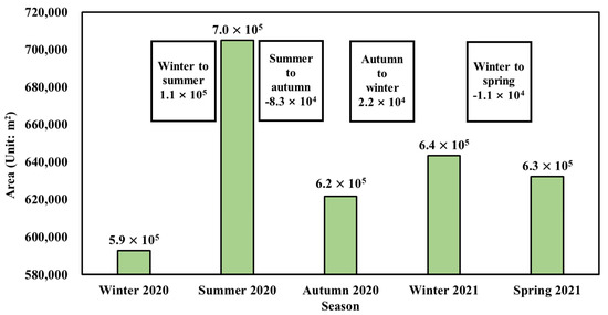
Figure 11.
Seagrass seasonal area variation and recovery. The area recovered by 5.0 × 10⁴ m2 after the occurrence of the No. 19 Typhoon in one year.
We compared seagrass meadow areas in winter 2021 derived from the application of the FPN and U-Net models and ground truth data, which were estimated to be 6.6 × 10⁵, 6.7 × 10⁵, and 6.4 × 10⁵ m2, respectively. The FPN results were found to be more consistent with the ground truth data than the U-Net results.
4. Discussion
This study was conducted to assess FPN performance for classifying subtidal and intertidal seagrass orthophotos by conducting various input data set preprocessing experiments and by setting hyper-parameters; U-Net processed with the same procedures was used for comparison. Seagrass is usually submerged in subtidal and intertidal areas; thus, sun glint and scattering occurring due to the presence of waves serve as challenges. To overcome such problems, preprocessing of input data sets, including adjustment of spatial resolution, the normalization of parameters, a combination of input data sets, and the selection of a suitable classification model, is essential. In our study, the optimal 2 m resolution, Gaussian blur radius of 901 (701 for U-Net), and data for the four seasons combination were determined, and FPN was found to outperform U-Net in the classification of subtidal and intertidal seagrass meadows.
The adjusted resolution images helped achieve better classification results than the original resolution image, which might be attributed to sun glint and scattering noise. Moreover, the computing time significantly increased with increasing image resolution. For optimal resolution images, the noise in images is averaged and merged with the surrounding pixels, reducing the learning time and increasing classification efficiency. This finding is consistent with that reported previously on image classification at different resolutions [57]. Under this condition, higher altitude drone missions and resampling of images into lower resolution could increase the efficiency. The trained model was designed to classify seagrass objects of different sizes in the resampled image. Although high-resolution drone photos were intended to obtain high-resolution seagrass mapping results automatically, we sacrificed the resolution for automatic high-accuracy classification, which may have led to information loss. For example, patches smaller than 2 m on the ground were averaged by the surrounding objects and not identified when images were resampled to 2 m for higher classification accuracy. Although they may not be essential in typical seagrass meadow for large area estimation, if small patch seagrass classification is essential in some case studies, we recommend compensating the FPN classification results by conducting additional unsupervised classification for small patches. Application of an appropriate Gaussian blur enables the achievement of higher classification accuracy. Gaussian blur may help further average out the surrounding pixels with noise (noise-induced wrong classification was reduced) and alleviate the brightness difference, increasing the texture homogeneity of seagrass and sediments and enabling learning through model application (wrong classification in sediments decreased). Application of Gaussian blur with an inappropriate radius may lead to the obtainment of different objects showing the same texture information or result in unsolved noises in orthophotos (see Table 3).
The classification accuracy was related to the input data set combinations. The input data set of the four seasons exhibited generalization ability and presented the most accurate classification results for the new data set. Although the three seasons data set achieved the same level of accuracy when applied to the new winter data set, because of the diversity of features, the four seasons data set should be selected, as seagrass shows different texture features in different seasons (Figure 12). Image texture could be identified and interpreted by humans but not by traditional classification methods [19]. However, the convolutions of the FPN extract the texture information automatically, and the training and classification of the classifier rely more on texture information than on other automatically extracted information [58,59]. Additionally, it is recommended that photos should be acquired under the conditions of different water levels, as it may also increase the contrast of texture feature difference.
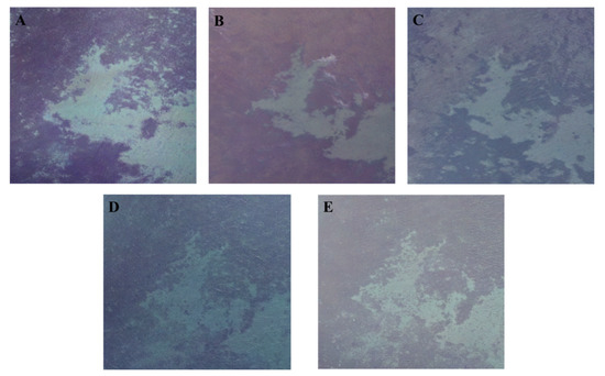
Figure 12.
The texture and color information comparison depicted for every season in one specific area: (A) 10 January 2020 winter, (B) 18 June 2020 summer, (C) 17 September 2020 autumn, (D) 11 December 2020 winter, and (E) 5 March 2021 spring.
FPN was found to demonstrate better classification accuracy for the new data set than U-Net when optimal preprocessing was conducted. The lower feature map of FPN was designed for small object detection in the image; its multi-layer structure helped efficiently classify objects of different sizes in different layers generated from the resampled image [28]. Additionally, the ResNet used in the FPN structure circumvents the gradient explosion, causing FPN to effectively learn the seagrass features even in deeper networks and to yield better classification results [60]. The worse results of the U-Net might be attributable to its learning for redundant features and ignoring of small objects [27,61]. Nevertheless, unsuccessful classification pixels existed in areas where a large brightness gradient appeared (e.g., sun glint, see Figure 13C) or the texture information in non-seagrass areas was similar to that in seagrass areas (Figure 13D). Successful classification results are often obtained in areas with relatively homogeneous texture or those surrounded by marked boundaries (Figure 13A,B). In addition, we found no significant difference in the classification results of seagrasses in the deep and shallow subtidal zones (Figure 14A,C), as the trained model might have learned adequate features to achieve highly accurate seagrass classification in different water depths. Moreover, the classification results showed lower accuracy for Z. japonica (Figure 14B) than for Z. marina (Figure 14A), possibly because of the insufficient training data set for Z. japonica. Apart from that, the bed with a homogenous texture yielded less wrong seagrass classification results than the bed with a heterogeneous texture (Figure 14C–E). More data augmentation and preprocessing procedures in low-accuracy areas may help improve classification accuracy.
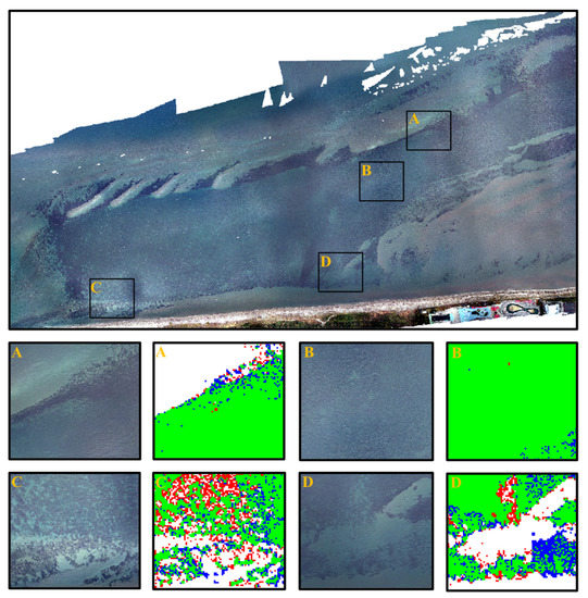
Figure 13.
Comparison of the classification results in different texture information: green, TP; blue, FP; red, FN; white, TN. (A) The clear boundary between seagrass and non-seagrass (high-accuracy classification). (B) The homogenous texture inside the seagrass (high-accuracy classification). (C) The remarkable light changes are attributable to the sun glint (low-accuracy classification). (D) The similar texture information for seagrass and non-seagrass (low-accuracy classification).
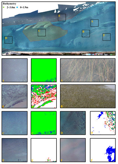
Figure 14.
Comparison of classification results at different depths and environments: green, TP; blue, FP; red, FN; white, TN. (A) The classification results for Z. marina (eelgrass) in the shallow subtidal zone (high-accuracy classification). (B) The classification results for Z. japonica (Japanese eelgrass) in the shallow subtidal zone (low-accuracy classification). (C) The classification results in the deep subtidal zone (high-accuracy classification). (D,F) The worse seagrass classification results in heterogeneous texture beds. (E) The less wrong seagrass classification results in the homogenous texture beds.
The seagrass area decreased significantly from summer to autumn, and it significantly increased from winter to summer. The information gap of the seagrass recovery after the typhoon was also filled, and 8% of the seagrass area recovered. The decrease in seagrass meadows may be related to the high sea surface temperature [62] and rapid temperature fluctuation [63]. The light intensity causes a seagrass net photosynthesis peak in spring, which promotes seagrass growth [64]. In addition, water depth [65], species [66], and meadow size [67] affect the variation, and the recovery process may be related to the stability of seagrass. To observe the differences in spatiotemporal variation and recovery among seagrass meadows, we selected three typical meadow size areas (areas 1, 2, and 3) according to the seagrass species, water depth, and meadow size (see Figure 15). Area 1 was occupied by large meadows in the deep subtidal zone, where the seagrass distribution was stable; area 2 was occupied by small Z. marina meadows in shallow subtidal zone; area 3 contained small Z. japonica meadows in the shallow subtidal zone, where significant variations were identified. For the three selected sites, the seagrass cover increased by 1% in area 1, 58% in area 2, and 30% in area 3 from winter 2020 to winter 2021. This result is consistent with that of a previous study showing that the asynchronous local dynamics of seagrass contribute to its stability [38].
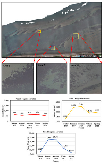
Figure 15.
Seagrass variation and recovery at the different selected areas (selection of the 2020 winter orthophoto as the base map to explain the location of the three areas).
To apply the model for classification in a new environment, such as the blue carbon assessment, annual monitoring in the most prosperous season (early summer at the study site) for seagrass is necessary, and our FPN model with the four seasons data set may be applicable for each new site without further tuning [68]. However, if the classification accuracy in a new environment is lower than expected, we recommend implementing transfer learning based on our tuned FPN model or collecting a new data set during an appropriate season. Establishment of a new FPN model using only the newly collected one-season data set with the same preprocessing procedures as our model may also be applicable for annual monitoring purposes. The results in Table 8 indicate that the trained FPN model based on a sufficient one season data set can be applied to the same season data set for annual monitoring with high classification accuracy.
Our trained model and proposed framework will facilitate classification of areas dominated by seagrass to obtain high-accuracy seagrass mapping results, which will help the observation of seasonal and unexpected event (typhoons or tsunamis)-induced variations in seagrass. Except for seagrass vegetation classification, this framework may also be applicable for classifying algae, rocks, and sediments. The training data set can be collected in cloudy or sunny weather with oblique photogrammetry and then processed using the same preprocessing to obtain the trained model for different targets. The collection frequency and time depend on whether the target varies in different seasons. In addition, the easily applied framework, including photo collection and classification procedures using FPN, can be helpful for the local coastal management office or NPO, who have limited access to the hyper-spectral or multi-spectral cameras for monitoring variations in benthic targets. The low cost of the equipment and lower computational resource consumption are other benefits for applying this framework in similar places.
5. Conclusions
We established an FPN-based classification method for drone photos of subtidal and intertidal seagrass meadows in the Futtsu tidal flat of Tokyo Bay, which demonstrated the first application of FPN for submerged seagrass classification. During model development, we considered the spatial resolution, normalization preprocessing, and suitable combination of seasonal input data sets. Using the four seasons data set with a 2 m resolution and processing with a Gaussian blur radius of 901, the FPN model achieved the highest accuracy with an OA of 0.957, precision of 0.895, recall of 0.942, F1-score of 0.918, and IoU of 0.848, ultimately outperforming the accuracy of the conventional U-Net-based model. Our method also overcame the difficulty of classifying submerged seagrass meadows under the influence of scattering due to the fact of waves and sun glint. As the model demonstrates a high generalization ability, it may be applicable to a new site without further tuning. The implementation of transfer learning or training of a new FPN model using an appropriate seasonal data set in a new site may be considered an option when the accuracy of the direct application of our FPN is insufficient. Thus, our model will contribute toward blue carbon assessment of local seagrass meadows. Our model and framework may facilitate seagrass classification in new areas. Applying the model to other submerged targets (e.g., algae, rocks, and sediments) may also be feasible.
The classification results of seagrass meadows in the Futtsu tidal flat of Tokyo Bay revealed seasonal changes in the detailed spatial distribution of the meadows. The seagrass area recovered by 8% after the occurrence of Typhoon No. 19 in 2019. This finding indicates that the proposed model is useful for understanding detailed spatiotemporal variations in seagrass meadows, which will help local management associations in assessing the blue carbon and devising effective management strategies, particularly for those associations that have limited access to hyper-spectral and multi-spectral equipment.
Author Contributions
Conceptualization, J.C. and J.S.; Data curation, J.C.; Formal analysis, J.C.; Funding acquisition, J.S.; Investigation, J.C.; Methodology, J.C. and J.S.; Resources, J.S.; Software, J.C.; Validation, J.C.; Visualization, J.C.; Writing—original draft, J.C.; Writing—review and editing, J.S. All authors have read and agreed to the published version of the manuscript.
Funding
This study was partially supported by an FY2019-2020 Research Grant from the Japanese Institute of Fisheries Infrastructure and Communities (grant number: 9467) and JSPS KAKENHI (grant number: JP20H02250).
Institutional Review Board Statement
Not applicable.
Informed Consent Statement
Not applicable.
Data Availability Statement
The data presented in this study are available upon request from the corresponding author.
Acknowledgments
The computations were carried out using the computer resources offered under the category of General Projects by the Research Institute for Information Technology, Kyushu University. The authors would like to acknowledge Zhiling Guo, Peiran Li, Xiaodan Shi, and Suxing Lyu (Center for Spatial Information Science, The University of Tokyo) for their enlightening conversations and thank the anonymous reviewers for their helpful comments on the first version of this manuscript.
Conflicts of Interest
The authors declare no conflict of interest.
References
- Kuwae, T.; Hori, M. Blue Carbon in Shallow Coastal Ecosystems. Blue Carbon Shallow Coast. Ecosyst. 2019, 1, 10. [Google Scholar] [CrossRef]
- Macreadie, P.I.; Anton, A.; Raven, J.A.; Beaumont, N.; Connolly, R.M.; Friess, D.A.; Kelleway, J.J.; Kennedy, H.; Kuwae, T.; Lavery, P.S.; et al. The future of Blue Carbon science. Nat. Commun. 2019, 10, 3998. [Google Scholar] [CrossRef] [Green Version]
- Kendrick, G.A.; Aylward, M.J.; Hegge, B.J.; Cambridge, M.L.; Hillman, K.; Wyllie, A.; Lord, D.A. Changes in seagrass coverage in Cockburn Sound, Western Australia between 1967 and 1999. Aquat. Bot. 2002, 73, 75–87. [Google Scholar] [CrossRef]
- Jordà, G.; Marbà, N.; Duarte, C.M. Mediterranean seagrass vulnerable to regional climate warming. Nat. Clim. Chang. 2012, 2, 821–824. [Google Scholar] [CrossRef] [Green Version]
- Arias-Ortiz, A.; Serrano, O.; Masqué, P.; Lavery, P.S.; Mueller, U.; Kendrick, G.A.; Rozaimi, M.; Esteban, A.; Fourqurean, J.W.; Marbà, N.; et al. A marine heatwave drives massive losses from the world’s largest seagrass carbon stocks. Nat. Clim. Chang. 2018, 8, 338–344. [Google Scholar] [CrossRef] [Green Version]
- Oprandi, A.; Mucerino, L.; De Leo, F.; Bianchi, C.N.; Morri, C.; Azzola, A.; Benelli, F.; Besio, G.; Ferrari, M.; Montefalcone, M. Effects of a severe storm on seagrass meadows. Sci. Total Environ. 2020, 748, 141373. [Google Scholar] [CrossRef]
- Whanpetch, N.; Nakaoka, M.; Mukai, H.; Suzuki, T.; Nojima, S.; Kawai, T.; Aryuthaka, C. Temporal changes in benthic communities of seagrass beds impacted by a tsunami in the Andaman Sea, Thailand. Estuar. Coast. Shelf Sci. 2010, 87, 246–252. [Google Scholar] [CrossRef]
- Rozaimi, M.; Fairoz, M.; Hakimi, T.M.; Hamdan, N.H.; Omar, R.; Ali, M.M.; Tahirin, S.A. Carbon stores from a tropical seagrass meadow in the midst of anthropogenic disturbance. Mar. Pollut. Bull. 2017, 119, 253–260. [Google Scholar] [CrossRef]
- Dat Pham, T.; Xia, J.; Thang Ha, N.; Tien Bui, D.; Nhu Le, N.; Tekeuchi, W. A review of remote sensing approaches for monitoring blue carbon ecosystems: Mangroves, seagrasses and salt marshes during 2010–2018. Sensors 2019, 19, 1933. [Google Scholar] [CrossRef] [PubMed] [Green Version]
- Ruiz, H.; Ballantine, D.L. Occurrence of the seagrass Halophila stipulacea in the tropical west Atlantic. Bull. Mar. Sci. 2004, 75, 131–135. [Google Scholar]
- Moore, K.A.; Wilcox, D.J.; Orth, R.J. Analysis of the abundance of submersed aquatic vegetation communities in the Chesapeake Bay. Estuaries 2000, 23, 115–127. [Google Scholar] [CrossRef]
- Phinn, S.; Roelfsema, C.; Dekker, A.; Brando, V.; Anstee, J. Mapping seagrass species, cover and biomass in shallow waters: An assessment of satellite multi-spectral and airborne hyper-spectral imaging systems in Moreton Bay (Australia). Remote Sens. Environ. 2008, 112, 3413–3425. [Google Scholar] [CrossRef]
- Fornes, A.; Basterretxea, G.; Orfila, A.; Jordi, A.; Alvarez, A.; Tintore, J. Mapping Posidonia oceanica from IKONOS. ISPRS J. Photogramm. Remote Sens. 2006, 60, 315–322. [Google Scholar] [CrossRef]
- Wabnitz, C.C.; Andréfouët, S.; Torres-Pulliza, D.; Müller-Karger, F.E.; Kramer, P.A. Regional-scale seagrass habitat mapping in the Wider Caribbean region using Landsat sensors: Applications to conservation and ecology. Remote Sens. Environ. 2008, 112, 3455–3467. [Google Scholar] [CrossRef]
- Greene, A.; Rahman, A.F.; Kline, R.; Rahman, M.S. Side scan sonar: A cost-efficient alternative method for measuring seagrass cover in shallow environments. Estuar. Coast. Shelf Sci. 2018, 207, 250–258. [Google Scholar] [CrossRef]
- Wang, C.K.; Philpot, W.D. Using airborne bathymetric lidar to detect bottom type variation in shallow waters. Remote Sens. Environ. 2007, 106, 123–135. [Google Scholar] [CrossRef]
- Nahirnick, N.K.; Reshitnyk, L.; Campbell, M.; Hessing-Lewis, M.; Costa, M.; Yakimishyn, J.; Lee, L. Mapping with confidence; delineating seagrass habitats using Unoccupied Aerial Systems (UAS). Remote Sens. Ecol. Conserv. 2019, 5, 121–135. [Google Scholar] [CrossRef]
- Nababan, B.; Mastu, L.O.K.; Idris, N.H.; Panjaitan, J.P. Shallow-Water Benthic Habitat Mapping Using Drone with Object Based Image Analyses. Remote Sens. 2021, 13, 4452. [Google Scholar] [CrossRef]
- Duffy, J.P.; Pratt, L.; Anderson, K.; Land, P.E.; Shutler, J.D. Spatial assessment of intertidal seagrass meadows using optical imaging systems and a lightweight drone. Estuar. Coast. Shelf Sci. 2018, 200, 169–180. [Google Scholar] [CrossRef]
- Kim, H.K.; Kim, Y.; Lee, S.; Min, S.; Bae, J.Y.; Choi, J.W.; Park, J.; Jung, D.; Yoon, S.; Kim, H.H. SpCas9 activity prediction by DeepSpCas9, a deep learning–based model with high generalization performance. Sci. Adv. 2019, 5, eaax9249. [Google Scholar] [CrossRef] [PubMed] [Green Version]
- Yamakita, T. Eelgrass Beds and Oyster Farming in a Lagoon Before and After The Great East Japan Earthquake of 2011: Potential for Applying Deep Learning at a Coastal Area. In Proceedings of the IGARSS 2019—2019 IEEE International Geoscience and Remote Sensing Symposium, Yokohama, Japan, 28 July–2 August 2019; IEEE: Piscataway, NJ, USA, 2019; pp. 9748–9751. [Google Scholar] [CrossRef]
- Dewi, C.; Chen, R.C.; Liu, Y.T.; Yu, H. Various generative adversarial networks model for synthetic prohibitory sign image generation. Appl. Sci. 2021, 11, 2913. [Google Scholar] [CrossRef]
- Moniruzzaman, M.; Islam, S.M.S.; Lavery, P.; Bennamoun, M. Faster R-CNN Based Deep Learning for Seagrass Detection from Underwater Digital Images. In Proceedings of the 2019 Digital Image Computing: Techniques and Applications (DICTA), Perth, WA, Australia, 2–4 December 2019; IEEE: Piscataway, NJ, USA, 2019; pp. 1–7. [Google Scholar] [CrossRef]
- Quan, L.; Feng, H.; Lv, Y.; Wang, Q.; Zhang, C.; Liu, J.; Yuan, Z. Maize seedling detection under different growth stages and complex field environments based on an improved Faster R–CNN. Biosyst. Eng. 2019, 184, 1–23. [Google Scholar] [CrossRef]
- Hobley, B.; Arosio, R.; French, G.; Bremner, J.; Dolphin, T.; Mackiewicz, M. Semi-supervised segmentation for coastal monitoring seagrass using RPA imagery. Remote Sens. 2021, 13, 1741. [Google Scholar] [CrossRef]
- Jeon, E.-I.; Kim, S.-H.; Kim, B.-S.; Park, K.-H.; Choi, O.-I. Semantic Segmentation of Drone Imagery Using Deep Learning for Seagrass Habitat Monitoring. Korean J. Remote Sens. 2020, 36, 199–215. [Google Scholar] [CrossRef]
- Cheng, Z.; Qu, A.; He, X. Contour-aware semantic segmentation network with spatial attention mechanism for medical image. Vis. Comput. 2021, 1–14. [Google Scholar] [CrossRef] [PubMed]
- Jonathan, H. Understanding Feature Pyramid Networks for Object Detection (FPN). 2018. Available online: https://jonathan-hui.medium.com/understanding-feature-pyramid-networks-for-object-detection-fpn-45b227b9106c (accessed on 13 September 2021).
- Koo, K.M.; Cha, E.Y. Image recognition performance enhancements using image normalization. Hum.-Centric Comput. Inf. Sci. 2017, 7, 33. [Google Scholar] [CrossRef] [Green Version]
- Atkinson, P.M. Selecting the spatial resolution of airborne MSS imagery for small-scale agricultural mapping. Int. J. Remote Sens. 1997, 18, 1903–1917. [Google Scholar] [CrossRef]
- Kannojia, S.P.; Jaiswal, G. Effects of Varying Resolution on Performance of CNN based Image Classification An Experimental Study. Int. J. Comput. Sci. Eng. 2018, 6, 451–456. [Google Scholar] [CrossRef]
- Zhang, W.; Zhao, X.; Morvan, J.M.; Chen, L. Improving Shadow Suppression for Illumination Robust Face Recognition. IEEE Trans. Pattern Anal. Mach. Intell. 2019, 41, 611–624. [Google Scholar] [CrossRef] [Green Version]
- Tian, J.; Li, X.; Duan, F.; Wang, J.; Ou, Y. An efficient seam elimination method for UAV images based on Wallis dodging and Gaussian distance weight enhancement. Sensors 2016, 16, 662. [Google Scholar] [CrossRef]
- Su, J.M.; Liu, L.L.; Wan, Q.T.; Yang, Y.Z.; Li, F.F. Dehazing research on brightness equalization model of drone image. Int. Arch. Photogramm. Remote Sens. Spat. Inf. Sci. 2020, 42, 1289–1294. [Google Scholar] [CrossRef] [Green Version]
- Yin, H.; Gai, K.; Wang, Z. A Classification Algorithm Based on Ensemble Feature Selections for Imbalanced-Class Dataset. In Proceedings of the 2016 IEEE 2nd International Conference on Big Data Security on Cloud (BigDataSecurity), IEEE International Conference on High Performance and Smart Computing (HPSC), and IEEE International Conference on Intelligent Data and Security (IDS), New York, NY, USA, 9–10 April 2016; pp. 245–249. [Google Scholar] [CrossRef]
- Yamakita, T. Long-term spatial dynamics of a seagrass bed on Futtsu tidal flat in Tokyo Bay. Jpn. J. Conserv. Ecol. 2005, 10, 129–138. [Google Scholar]
- Shimozono, T.; Tajima, Y.; Kumagai, K.; Arikawa, T.; Oda, Y.; Shigihara, Y.; Mori, N.; Suzuki, T. Coastal impacts of super typhoon Hagibis on Greater Tokyo and Shizuoka areas, Japan. Coast. Eng. J. 2020, 62, 129–145. [Google Scholar] [CrossRef]
- Yamakita, T.; Watanabe, K.; Nakaoka, M. Asynchronous local dynamics contributes to stability of a seagrass bed in Tokyo Bay. Ecography 2011, 34, 519–528. [Google Scholar] [CrossRef]
- Japan Coast Guard Sea Chart of Tokyo Bay. 2020. Available online: https://www.kaiho.mlit.go.jp/e/index_e.html (accessed on 2 June 2021).
- Casella, E.; Collin, A.; Harris, D.; Ferse, S.; Bejarano, S.; Parravicini, V.; Hench, J.L.; Rovere, A. Mapping coral reefs using consumer-grade drones and structure from motion photogrammetry techniques. Coral Reefs 2017, 36, 269–275. [Google Scholar] [CrossRef]
- Sekrecka, A.; Wierzbicki, D.; Kedzierski, M. Influence of the sun position and platform orientation on the quality of imagery obtained from unmanned aerial vehicles. Remote Sens. 2020, 12, 1040. [Google Scholar] [CrossRef] [Green Version]
- Overstreet, B.T.; Legleiter, C.J. Removing sun glint from optical remote sensing images of shallow rivers. Earth Surf. Process. Landf. 2017, 42, 318–333. [Google Scholar] [CrossRef]
- Ortega-Terol, D.; Hernandez-Lopez, D.; Ballesteros, R.; Gonzalez-Aguilera, D. Automatic hotspot and sun glint detection in UAV multispectral images. Sensors 2017, 17, 2352. [Google Scholar] [CrossRef] [Green Version]
- Phantom 4 Pro—Product Information—DJI. 2021. Available online: https://www.dji.com/sg/phantom-4-pro/info#specs (accessed on 8 November 2021).
- Japan Meteoriological Agency Tidal Level Data in Kisarazu. 2021. Available online: https://www.data.jma.go.jp/gmd/kaiyou/db/tide/suisan/suisan.php?stn=KZ (accessed on 21 July 2021).
- Agisoft LLC Agisoft Metashape. 2021. Available online: https://www.agisoft.com/ (accessed on 6 May 2021).
- Yan, L.; Roy, D.P.; Zhang, H.; Li, J.; Huang, H. An automated approach for sub-pixel registration of Landsat-8 Operational Land Imager (OLI) and Sentinel-2 Multi Spectral Instrument (MSI) imagery. Remote Sens. 2016, 8, 520. [Google Scholar] [CrossRef] [Green Version]
- Li, M.; Han, S.; Shi, J. An enhanced ISODATA algorithm for recognizing multiple electric appliances from the aggregated power consumption dataset. Energy Build. 2017, 140, 305–316. [Google Scholar] [CrossRef]
- Lin, T.Y.; Dollár, P.; Girshick, R.; He, K.; Hariharan, B.; Belongie, S. Feature pyramid networks for object detection. In Proceedings of the 2017 IEEE Conference on Computer Vision and Pattern Recognition (CVPR), Honolulu, HI, USA, 21–26 July 2017; pp. 936–944. [Google Scholar] [CrossRef] [Green Version]
- Li, X.; Lai, T.; Wang, S.; Chen, Q.; Yang, C.; Chen, R. Weighted feature pyramid networks for object detection. In Proceedings of the 2019 IEEE International Conference on Parallel & Distributed Processing with Applications, Big Data & Cloud Computing, Sustainable Computing & Communications, Social Computing & Networking (ISPA/BDCloud/SocialCom/SustainCom), Xiamen, China, 16–18 December 2019; pp. 1500–1504. [Google Scholar] [CrossRef]
- Ronneberger, O.; Fischer, P.; Brox, T. U-Net: Convolutional Networks for Biomedical Image Segmentation. In Proceedings of the Medical Image Computing and Computer-Assisted Intervention—MICCAI 2015, Munich, Germany, 5–9 October 2015; Volume 9351, pp. 234–241. [Google Scholar]
- Chen, W.; Liu, B.; Peng, S.; Sun, J.; Qiao, X. S3D-UNET: Separable 3D U-Net for Brain Tumor Segmentation. In Proceedings of the Lecture Notes in Computer Science (Including Subseries Lecture Notes in Artificial Intelligence and Lecture Notes in Bioinformatics), Granada, Spain, 16 September 2018; Springer: Berlin/Heidelberg, Germany, 2019; Volume 11384, pp. 358–368. [Google Scholar] [CrossRef]
- Zhang, X.; Chen, X.; Yao, L.; Ge, C.; Dong, M. Deep neural network hyperparameter optimization with orthogonal array tuning. In Proceedings of the Communications in Computer and Information Science, Sydney, NSW, Australia, 12–15 December 2019; Springer: Berlin/Heidelberg, Germany, 2019; Volume 1142, pp. 287–295. [Google Scholar] [CrossRef] [Green Version]
- Wu, G.; Shao, X.; Guo, Z.; Chen, Q.; Yuan, W.; Shi, X.; Xu, Y.; Shibasaki, R. Automatic building segmentation of aerial imagery usingmulti-constraint fully convolutional networks. Remote Sens. 2018, 10, 407. [Google Scholar] [CrossRef] [Green Version]
- Guo, Z.; Wu, G.; Song, X.; Yuan, W.; Chen, Q.; Zhang, H.; Shi, X.; Xu, M.; Xu, Y.; Shibasaki, R.; et al. Super-resolution integrated building semantic segmentation for multi-source remote sensing imagery. IEEE Access 2019, 7, 99381–99397. [Google Scholar] [CrossRef]
- Liu, M.; Yu, T.; Gu, X.; Sun, Z.; Yang, J.; Zhang, Z.; Mi, X.; Cao, W.; Li, J. The Impact of Spatial Resolution on the Classification of Vegetation Types in Highly Fragmented Planting Areas Based on Unmanned Aerial Vehicle Hyperspectral Images. Remote Sens. 2020, 12, 146. [Google Scholar] [CrossRef] [Green Version]
- Meddens, A.J.H.; Hicke, J.A.; Vierling, L.A. Evaluating the potential of multispectral imagery to map multiple stages of tree mortality. Remote Sens. Environ. 2011, 115, 1632–1642. [Google Scholar] [CrossRef]
- Geirhos, R.; Rubisch, P.; Michaelis, C.; Bethge, M.; Wichmann, F.; Brendel, W. ImageNet-Trained CNNs Are Biased Towards Texture. In Proceedings of the Seventh International Conference on Learning Representations, New Orleans, LA, USA, 6–9 May 2019; pp. 1–20. [Google Scholar]
- Li, P.; Zhang, H.; Guo, Z.; Lyu, S.; Chen, J.; Li, W.; Song, X.; Shibasaki, R.; Yan, J. Understanding rooftop PV panel semantic segmentation of satellite and aerial images for better using machine learning. Adv. Appl. Energy 2021, 4, 100057. [Google Scholar] [CrossRef]
- Philipp, G.; Song, D.; Carbonell, J.G. Gradients explode—Deep Networks are shallow—ResNet explained. In Proceedings of the Sixth International Conference on Learning Representations, Vancouver, BC, Canada, 30 April–3 May 2018. [Google Scholar]
- Seo, H.; Huang, C.; Bassenne, M.; Xiao, R.; Xing, L. Modified U-Net (mU-Net) with Incorporation of Object-Dependent High Level Features for Improved Liver and Liver-Tumor Segmentation in CT Images. IEEE Trans. Med. Imaging 2020, 39, 1316–1325. [Google Scholar] [CrossRef] [PubMed] [Green Version]
- Strydom, S.; Murray, K.; Wilson, S.; Huntley, B.; Rule, M.; Heithaus, M.; Bessey, C.; Kendrick, G.A.; Burkholder, D.; Fraser, M.W.; et al. Too hot to handle: Unprecedented seagrass death driven by marine heatwave in a World Heritage Area. Glob. Chang. Biol. 2020, 26, 3525–3538. [Google Scholar] [CrossRef]
- Carlson, D.F.; Yarbro, L.A.; Scolaro, S.; Poniatowski, M.; McGee-Absten, V.; Carlson, P.R. Sea surface temperatures and seagrass mortality in Florida Bay: Spatial and temporal patterns discerned from MODIS and AVHRR data. Remote Sens. Environ. 2018, 208, 171–188. [Google Scholar] [CrossRef]
- Dennison, W.C. Effects of light on seagrass photosynthesis, growth and depth distribution. Aquat. Bot. 1987, 27, 15–26. [Google Scholar] [CrossRef]
- Xu, S.; Wang, P.; Wang, F.; Liu, P.; Liu, B.; Zhang, X.; Yue, S.; Zhang, Y.; Zhou, Y. In situ Responses of the Eelgrass Zostera marina L. to Water Depth and Light Availability in the Context of Increasing Coastal Water Turbidity: Implications for Conservation and Restoration. Front. Plant Sci. 2020, 11, 1933. [Google Scholar] [CrossRef] [PubMed]
- Grice, A.M.; Loneragan, N.R.; Dennison, W.C. Light intensity and the interactions between physiology, morphology and stable isotope ratios in five species of seagrass. J. Exp. Mar. Bio. Ecol. 1996, 195, 91–110. [Google Scholar] [CrossRef]
- Vidondo, B.; Duarte, C.M.; Middelboe, A.L.; Stefansen, K.; Lützen, T.; Nielsen, S.L. Dynamics of a landscape mosaic: Size and age distributions, growth and demography of seagrass Cymodocea nodosa patches. Mar. Ecol. Prog. Ser. 1997, 158, 131–138. [Google Scholar] [CrossRef] [Green Version]
- Neyshabur, B.; Bhojanapalli, S.; McAllester, D.; Srebro, N. Exploring generalization in deep learning. Adv. Neural Inf. Process. Syst. 2017, 2017, 5948–5957. [Google Scholar]
Publisher’s Note: MDPI stays neutral with regard to jurisdictional claims in published maps and institutional affiliations. |
© 2021 by the authors. Licensee MDPI, Basel, Switzerland. This article is an open access article distributed under the terms and conditions of the Creative Commons Attribution (CC BY) license (https://creativecommons.org/licenses/by/4.0/).