Article

Characterizing a Heavy Dust Storm Event in 2021: Transport, Optical Properties and Impact, Using Multi-Sensor Data Observed in Jinan, China

1
Key Laboratory of Atmospheric Optics, Anhui Institute of Optics and Fine Mechanics, Hefei Institutes of Physical Science, Chinese Academy of Sciences, Hefei 230031, China
2
Science Island Branch of Graduate School, University of Science and Technology of China, Hefei 230026, China
3
Atmospheric Sounding Technology Support Center of Shandong Meteorological Bureau, Jinan 250031, China
4
Advanced Laser Technology Laboratory of Anhui Province, Hefei 230037, China
5
Jinan Environmental Monitoring Center of Shandong Province, Jinan 250101, China
6
Shandong Meteorological Observatory, Jinan 250031, China
*
Author to whom correspondence should be addressed.
Remote Sens. 2022, 14(15), 3593; https://doi.org/10.3390/rs14153593
Submission received: 21 June 2022 / Revised: 20 July 2022 / Accepted: 25 July 2022 / Published: 27 July 2022
(This article belongs to the Special Issue Remote Sensing of Aerosols and Gases in Cities II)

Abstract

:
On 15 March 2021, the strongest sandstorm of the last 10 years occurred in China. The MODIS, MPL lidar, EDM 180, ADI 2080 and Meteorological observation instruments were used to observe the dust in Jinan, China, while the HYSPLIT model was also employed to find the source. It was found that the dust originated from Mongolia and the Gobi desert and was transported to Jinan at night on 14th March, lasting until the 18th. Multi-layer dust was observed, of which the dust below the height of 1 km was strongest with the VDR about 0.2 and the maximum extinction coefficient up to 3 km−1. The values of AOD and AE were greater than 2 and less than 0.25, respectively. The mass concentrations of PM10 and PM2.5 increased rapidly, and were up to 573 µg/m3 and 3406 µg/m3, respectively. Additionally, the mass concentration ratio decreased rapidly, with a minimum of 17%. The particle size of the dust was mainly distributed between 0.58–6.50 micros due to larger particles increasing dramatically; simultaneously, both the proportion and the value for calcium ions in PM2.5 went up. The dust had an obvious impact on the vertical structure of the air temperature, resulting in occurrence of a strong inversion layer.

Graphical Abstract

1. Introduction

Dust aerosols are emitted from eolian erosion over arid and semi-arid areas and are vertically injected into the atmosphere, traveling long distances [1]. In terms of aerosol dry mass, mineral dust is the most abundant component in atmospheric aerosol [2,3,4]. Through their radiative and cloud condensation nucleus effects, dust aerosols have a key role in the atmospheric radiation budget and hydrological cycles [2,5,6], and highly impact climate and environmental changes [7,8,9]. Meanwhile, dust particles pose a serious threat to the ecosystem [10] and human health [5,11,12,13,14].
At present, many previous studies have focused on dust aerosols, including observation and simulation, which are related to the formation mechanism, temporal and spatial distribution, optical properties, the dust source, the transport paths and their effects. Conventional meteorological data and satellite cloud image data are used to analyze the causes of dust weather in detail [1,15,16,17,18,19,20,21], which is conductive to improving the accuracy of the dust weather forecast. Through these analysis cases, we can summarize the occurrence and activity law of dust, find the forecast indexes, then provide scientific evidence and ideas for the forecast of dust weather. Satellite remote sensing data from active and passive sensors, such as the Cloud-Aerosol Lidar and Infrared Pathfinder Satellite Observation (CALIPSO) lidar (CALIOP), the Moderate Resolution Imaging Spectroradiometer (MODIS) and the Multi-Angle Imaging Spectrometer (MISR), are often used to study the temporal and spatial distribution of dust and to analyze the origin of dust [22,23,24,25,26]. There are also many ground-based monitoring tools for dust, such as lidar and a sun photometer. Lidar is generally used to obtain the vertical distribution, extinction coefficient and particle shape of dust [27,28,29,30,31,32,33], while a sun photometer is used to retrieve the optical thickness, single scattering albedo and particle size distribution of dust [34,35]. The particle concentration monitoring equipment has also been gradually used to observe the impact of dust on air quality in recent years. In addition, atmospheric chemical transport models are increasingly used in the study of dust [36,37]. However, the lack of observation constraints and other factors have brought uncertainties into the model estimate [38,39,40]. To reduce the uncertainties, comprehensive and multi-platform observations are necessary. Han et al. analyzed the optical properties, time–height distribution and impact on air quality of a dust event in Nanjing, China on 1 May 2011, with synergistic ground-based satellite sensors and a transport model [41]. Yoon et al. revealed two severe Asian dust events originating from the Taklimakan and Gobi deserts, based on a comprehensive approach that combines multiple satellite measurements, ground observations and model simulation [42]. Huang et al. analyzed the dust weather process in East Asia in May 2019 using space-borne and ground-based lidars [43].
On 15 March 2021, China witnessed the most severe dust weather process of the past decade. The peak concentration of PM10 in many places in northern China exceeded 5000 µg/m3, which was the highest value since 2013. According to the monitoring of the FY-4 meteorological satellite, the visible dust area reached 466,000 km2 at 08:00 on 15 March [44]. To assess the impacts of dust aerosol on radiation–cloud–climate and regional air quality, it is important to characterize this dust event. Shi et al. identified the sources of sand using radionuclides [45]. Yang et al. analyzed the causes of this dust weather by using the methods of synoptic analysis and physical quantity diagnosis. Liang et al. collected dust samples from nine cities and studied the process of dust emission and transport by analyzing the composition changes of dust substances [46]. However, the optical properties and influences of the dust have not been reported yet. The characteristics of this dust event are analyzed in this paper, using the data observed via lidar and other platforms in Jinan, the capital of Shandong Province. In the Section 2 of this paper, the instruments and methods are introduced. In the Section 3 of the paper, the observation results are analyzed and discussed, including time–height distribution, optical properties and the impact on temperature vertical structure and particle concentration. Lastly, the conclusions are summarized.

2. Instruments and Methods

2.1. Ground-Based Instruments

2.1.1. Micro Pulse Lidar—MPL

The lidar data are from the micro pulse lidar located in Huaiyin District of Jinan (116.81°E, 36.66°N). This lidar is a polarized Mie scattering lidar with an emission wavelength of 532 nm. The temporal and spatial resolution of lidar are 10 min and 15 m, respectively. During the observation, the lidar is operated continuously in vertical pointing mode. The observation blind zone of this lidar is 75 m, so the data below 0.1 km are not analyzed in this paper. Two types of products from the lidar, i.e., the extinction coefficient and the volume depolarization ratio (VDR), are used in this paper. The extinction coefficient is obtained by solving the lidar equation using the Fernald method, whose value reflects the degree of particulate pollution. The larger the value, the more serious the pollution is. The VDR is obtained by multiplying the ratio of a parallel component and the perpendicular component from the backscattering signal by the gain constant of two channels. The value of VDR reflects the non-spherical characteristics of aerosol particles, which are often used to distinguish dust and urban pollutants [31,47].

2.1.2. Environmental Dust Monitor-EDM 180

The particle concentration data are from the device EDM 180 installed on Guishan, Jinan (117.01°E, 36.60°N). The EDM 180 is designed and manufactured by Grimm Aerosol Technik company in Germany, which is used for continuous measurement of airborne dust and its particle size distribution. The measuring principle of the instrument is based on light scattering, and the light source is a semiconductor laser with a wavelength of 685 nm. According to the correlation between scattered light intensity and particle size, the electric signal of the diode will be classified into 31 different size channels (as shown in Table 1) after an adequate amplification. Then, the number of particles in each channel can be obtained by calculating the magnitude of scattered light intensity in this channel.

2.1.3. Monitor for Aerosols and Gases in Ambient Air—ADI 2080

In order to analyze the changes in aerosol particle composition in dust weather, the mass concentration data of soluble ions in PM2.5 observed by Monitor for Aerosols and Gases in ambient Air (MARGA) located in Shandong Jianzhu University (117.19°E, 36.68°N) were analyzed. MARGA is jointly developed by Metrohm Applikon company and Energy Research Center of the Netherlands, and is composed of a sampling system, an analysis system and an integrated control system. The instrument adopts a unique sampling device to absorb the gas and aerosol into the water phase, respectively, and separate them from each other. Then, the solution is analyzed using an ion chromatography method to obtain the composition of gas and water-soluble ions in the aerosol. The measured results output by the instrument include the mass concentration of gases (HCl, HNO2, HNO3, SO2 and NH3) and the water-soluble ions (Cl, NO3, SO42−, NH4+, Na+, K+, Ca2+ and Mg2+) in PM2.5.

2.2. Satellite Remote Sensing Instrument-MODIS

MODIS is a large space remote sensing instrument developed by National Aeronautics and Space Administration (NASA). It was launched with Terra Am satellite in 1999 and with Aqua PM satellite in 2002. MODIS multi-band data can simultaneously provide information reflecting the characteristics of land surface conditions, cloud boundary, cloud characteristics, ocean water color, phytoplankton, biogeography, chemistry, atmospheric water vapor, aerosol, surface temperature, cloud top temperature, atmospheric temperature, ozone and cloud-top height. The MODIS level-2 atmospheric aerosol product (04_L2) provides full global coverage of aerosol properties from the Dark Target (DT) and Deep Blue (DB) algorithms. “Fine” aerosols (anthropogenic pollution) and “coarse” aerosols (natural particles, e.g., dust) are also derived. Level-2 AOD and the Angstrom exponent (Collection 6.0, spatial resolution 10 × 10 km, DB algorithm) are used in this study [48]. In general, the Angstrom exponent ranges from 0.0 to 2.0, with smaller Angstrom exponents corresponding to larger aerosol particle sizes, often used to identify pollution and dust.

2.3. Backward Trajectory Modeling System-HYSPLIT

The Hybrid Single-Particle Lagrangian Integrated Trajectory Model (HYSPLIT) continues to be one of the most extensively used atmospheric transport and dispersion models in the atmospheric sciences community [49]. It was jointly developed by the National Oceanic and Atmospheric Administration (NOAA) Air Resources Laboratory (ARL) and the Australian Meteorological Administration (AMA). The model calculation method is a hybrid between the Lagrangian approach, using a moving frame of reference for the advection and diffusion calculations as the trajectories or air parcels move from their initial location, and the Eulerian methodology, which uses a fixed three-dimensional grid as a frame of reference to compute pollutant air concentrations [47]. The model can be run interactively on the Web through the Real-time Environmental Applications and Display System (READY, http://www.ready.noaa.gov, accessed on 15 March 2021) [50], or installed on PC and run using a graphical user interface (GUI). In order to trace the source of the dust, we chose READY, which has been continuously maintained and expanded since 1997 and currently uses the HYSPLIT version January 2022 Revision (V5.2.0), as the tool to calculate the backward trajectory of air mass in the paper.
In HYSPLIT model, the computation of the new position at a time step ( Δ t ) due to the mean advection by the wind determines the trajectory that a particle or puff will follow [49]. In the other words, the change in the position vector P with time is computed from the average of the three-dimensional velocity vectors V at their initial position P ( t ) and first-guess position P ( t + Δ t ) [51]. The final position is
P ( t + Δ t ) = P ( t ) + 0.5 [ V ( P , t ) + V ( P , t + Δ t ) ] Δ t
and the first guess position is
P ( t + Δ t ) = P ( t ) + V ( P , t ) Δ t
In addition, the ground meteorological observation data (temperature, pressure and relative humidity) and temperature profile data are also used in the paper. The ground meteorological observation data are from Jinan national basic meteorological station (117.01°E, 36.60°N, 170.3 m above sea level), while the temperature profile data are taken from Zhangqiu radiosonde station (117.52°E, 36.65°N, 264.2 m above sea level).

3. Results and Discussion

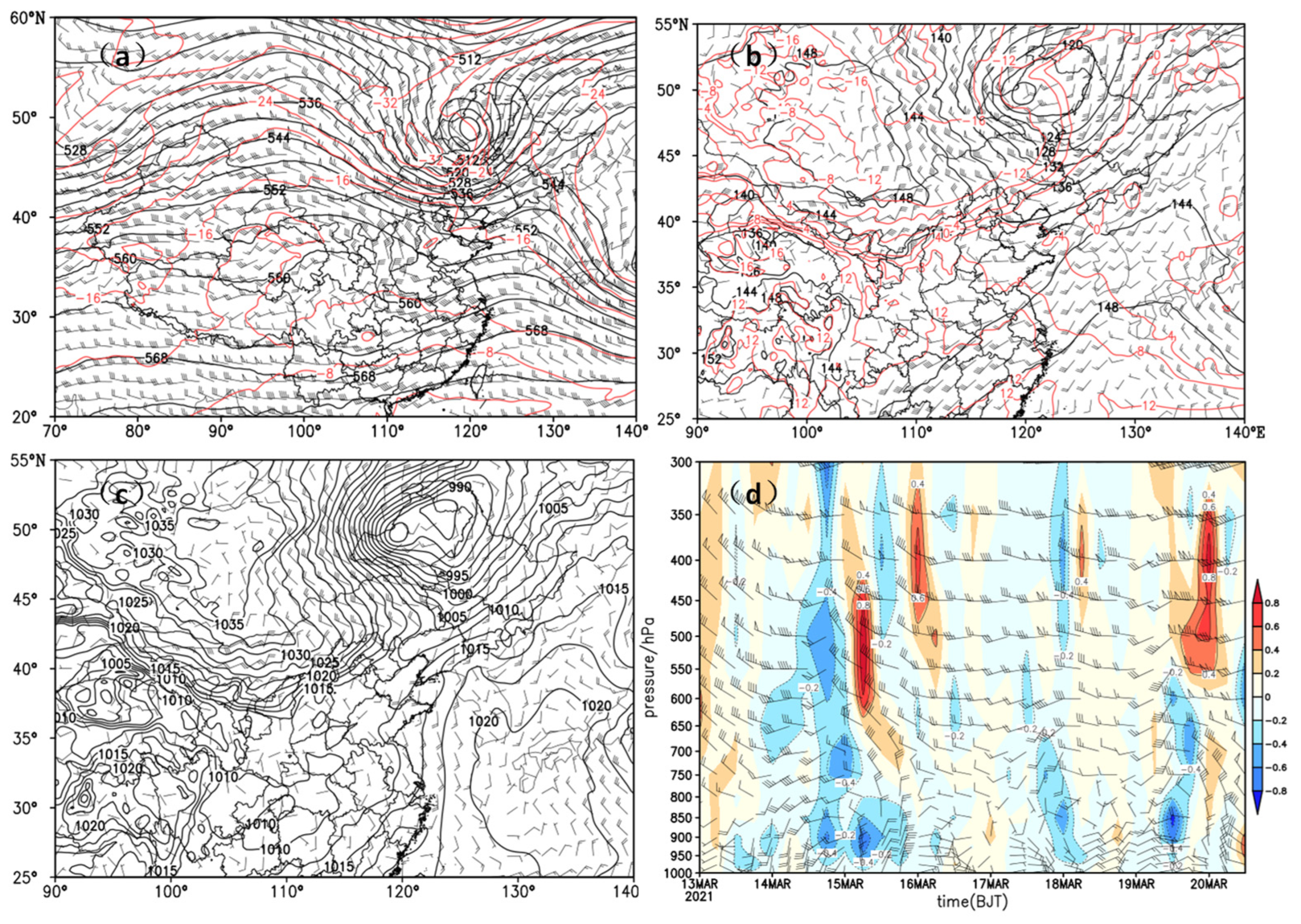
3.1. Weather Process

The Mongolian cyclone began to develop near the Altai mountain and then gradually moved eastward and strengthened on 13 March 2021. At 17:00 on 14 March, the cyclone center reached the east of Mongolia, with the strongest development, and the central pressure was lower than 985 hpa. Under the strong cyclone, a large amount of dust in Mongolia was drawn into the upper air and moved eastward and southward with the cold high pressure at the back of the cyclone, affecting most areas of northern China. Figure 1 displayed the Mongolian cyclone observed by FY-4A satellite.
On 15 March, the air over Jinan was controlled by northwest air flow, and the near ground was affected by cold air and was in front of high pressure (as shown in Figure 2a–c). Affected by the transport and deposition of high-altitude dust, the mass concentration of PM10 in Jinan increased rapidly. From the 16th to the 18th, the atmosphere over Jinan remained static and stable with flat circulation and weak vertical movement (as shown in Figure 2d). On the 17th, the unsettled dust in the downstream area flowed back, under the influence of southerly air flow in the middle and lower layers and weak southeast wind near the ground. The air quality became good due to the effect of wet deposition on the 18th, and the dust intrusion process ended.

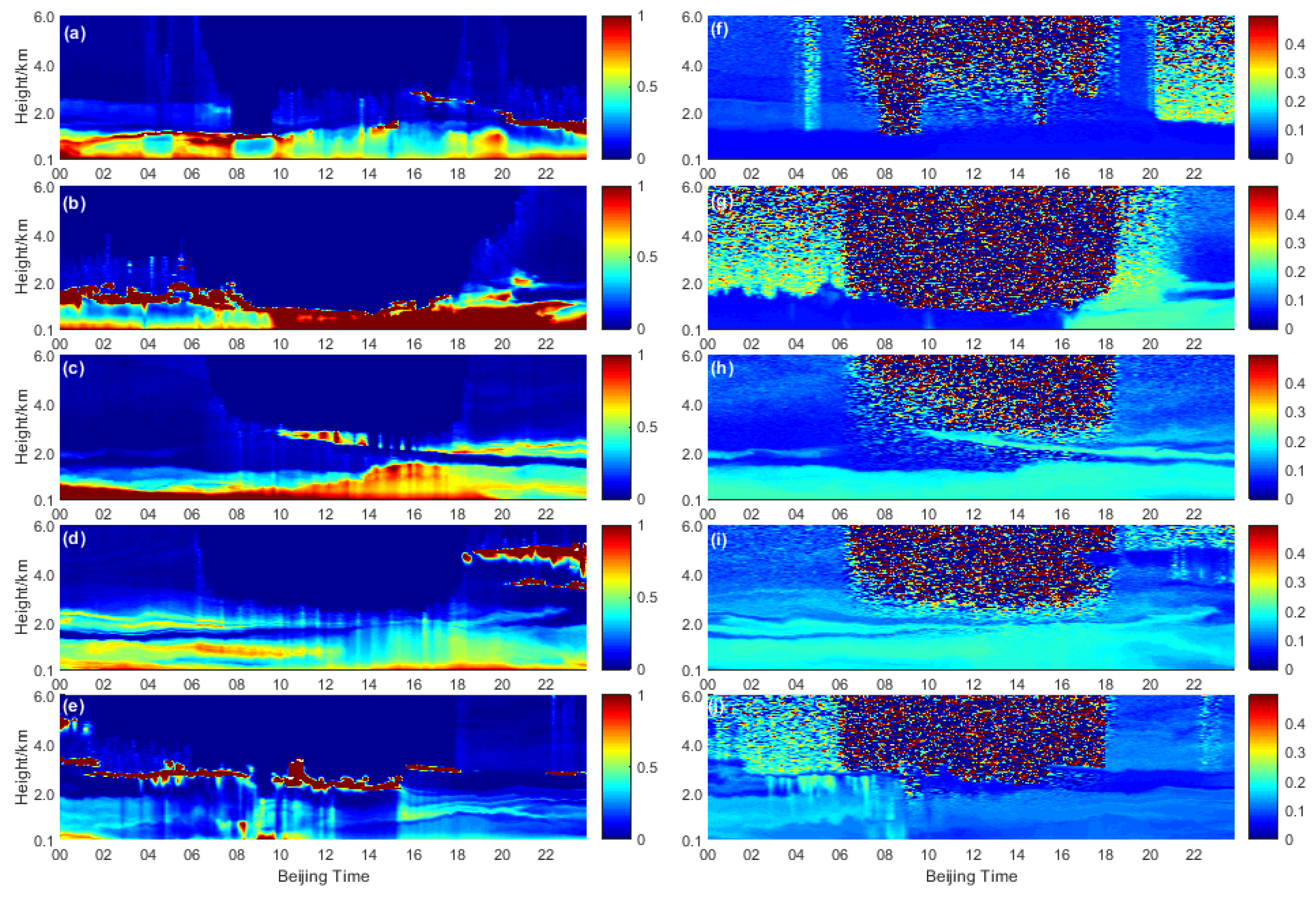
3.2. Optical Properties and Time–Height Evolution

Figure 3 illustrates the time series of the extinction coefficient and the VDR profiles in Jinan from 14–18 March 2021. It is shown that a thin pollution layer near 2 km was observed by the lidar system at about 20:00 on 14 March. Both the extinction coefficient (>1 km−1) and the VDR (>0.2) values were large, indicating the dust intrusion. From 10:00 to 16:00 on the 15th, there was serious urban aerosol pollution, with a large extinction coefficient (>1 km−1) but small VDR (<0.1). Because the laser cannot penetrate the urban aerosols pollution layer, the dust layer near 2 km could not be observed during this period. At about 16:00 on the 15th, due to the combined action of low-level transport and dry deposition, there was dust from near ground to 2 km height. At 02:00 on the 18th, the extinction coefficient decreased to less than 0.5 km−1, indicating that the dust was very weak. By 09:00, the VDR decreased to about 0.1, marking the end of the dust intrusion process.
It is worth noting that the phenomenon of multi-layer dust is observed. They are 1 km layer, 2 km layer and 3 km layer, respectively. The duration of the 1 km layer that is from near ground to 1 km height, was the longest. From 20:00 on the 15th to 06:00 on the 16th, there was a thin dust layer at an altitude of about 2 km; that is, a 2 km layer. The extinction coefficient of this layer was not so large, indicating that the amount of dust was not so large. At about 10:00 on the 16th, a very strong dust layer was observed between 2–3 km; that is, a 3 km layer. The height of this layer continued to decline, dropped to about 2 km at 18:00 on the 16th and merged with 1 km dust layer at 12:00 on the 17th.
Figure 4 gives the vertical profiles of the extinction coefficient and the VDR at several typical moments. The phenomenon of “multi-layer dust” previously described can be clearly seen from the figure. In addition, at these time points, the values for VDR of the dust layer are around 0.2, but the extinction coefficient decreases with time.
The time series of extinction coefficient and VDR at the heights of 510 m, 1005 m, 2010 m and 3000 m are given in Figure 5 to better analyze the dust intruding process. It can be seen that the dust at the height of 510 m and 1005 m was relatively stable, existing from the beginning to the end, and the VDR was stable at about 0.2. The dust lifting shows two periods at the height of 2010 m. One happened from 20:00 on the 14th to 06:00 on the 15th, and the other happened from 18:00 on the 16th to 18:00 on the 17th. The average value for VDR during these two periods was 0.23 and 0.15, respectively. There was a dust layer at the height of 3000 m from 18:00 on the 16th to 06:00 on the 17th. The average value for VDR was 0.13, which was lesser than that at the heights of 510 m, 1005 m and 2010 m, indicating that the dust particles transported at this height are smaller than those in the lower layers.
Figure 6 depicts the curve of the extinction coefficient at 495 m and the mass concentration of ground PM10 with time. It can be seen that the changing trend is basically in line, but the change in ground PM10 mass concentration (with the maximum value lager than 3000 µg/m3) is later than the change in the extinction coefficient at 495 m (with the maximum value larger than 2.5 km−1).

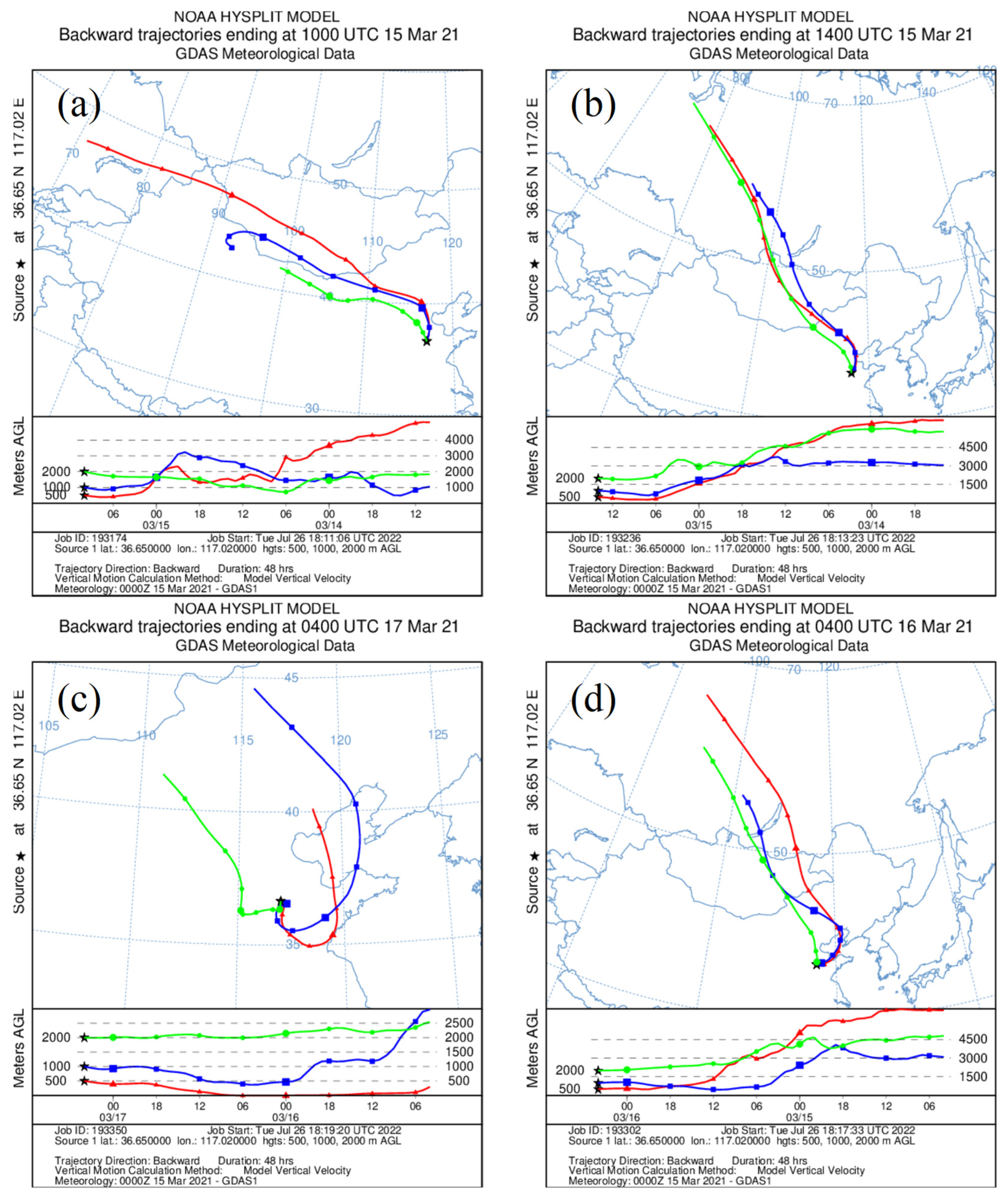
3.3. Transport Paths

To analyze the source and transport of the dust, the backward trajectories of air mass during the dust-affected period were calculated through READY, as shown in Figure 7. The meteorological data are Global Data Assimilation System (GDAS) data. The given location is Jinan (36.65°N, 117.02°E) and the calculated heights include 500 m, 1000 m and 2000 m. It can be seen from Figure 7a that the dust mainly came from the western region of Mongolia and the Gobi desert between China and Mongolia in the beginning. As time passed, the dust source transferred to the middle east region of Mongolia (as shown in Figure 7b,c). This result is consistent with the weather background of the Mongolia cyclone, which was moving southeast. By 12:00 on the 16th, the air mass changed from the northwest to the northeast in the Bohai Bay, and then affected Jinan. By 12:00 on the 17th, there was a back-flow southeast air mass at the height of 500 m and 1000 m, while the east air mass lay at the height of 2000 m.
Aqua-MODIS aerosol optical depth (AOD) and angstrom exponent (AE) are given in Figure 8 from 15 March to 18 March. We can see that large value for AOD (>2) and small value for AE (<0.25) are illustrated over the upper reaches of Shandong on 15 March, indicating that coarse-mode particles were dominant. The AOD in most areas of Shandong (except peninsula area) was greater than 0.75 and the AE was less than 0.25 on 16 March, indicating that dust affected Shandong, but the intensity weakened. The dust continued to affect most parts of Shandong on 17 March, but began to dissipate in southern Shandong. No aerosol pollution was retrieved in Shandong on 18 March, meaning that the impact of the dust process on Shandong ended or was very weak. This result is consistent with the result of weather analysis. Unfortunately, due to the limitations of observation time and the occurrence of clouds, MODIS data cannot reflect the origin of the dust and the process that began to affect Shandong.

3.4. Dust Impacts

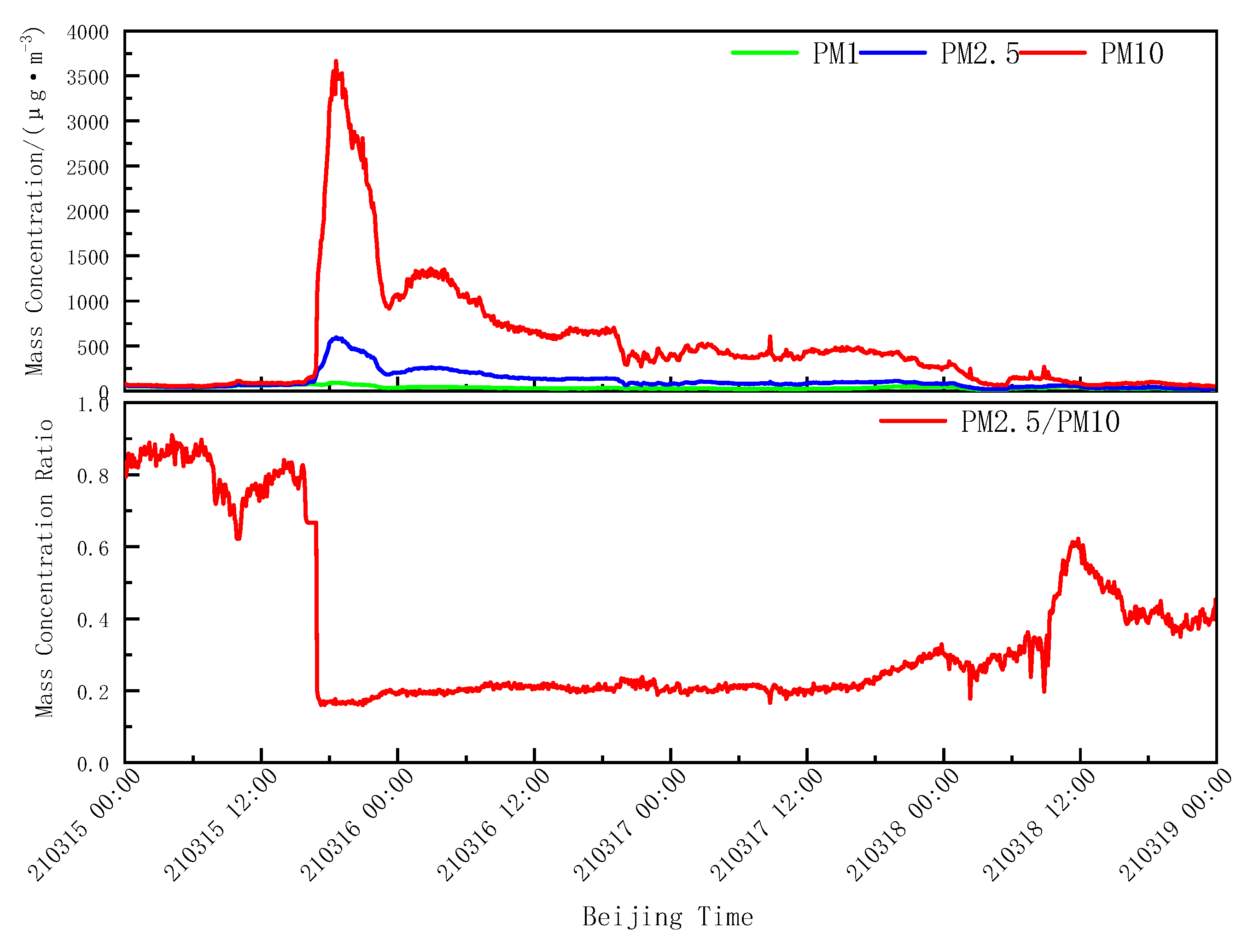
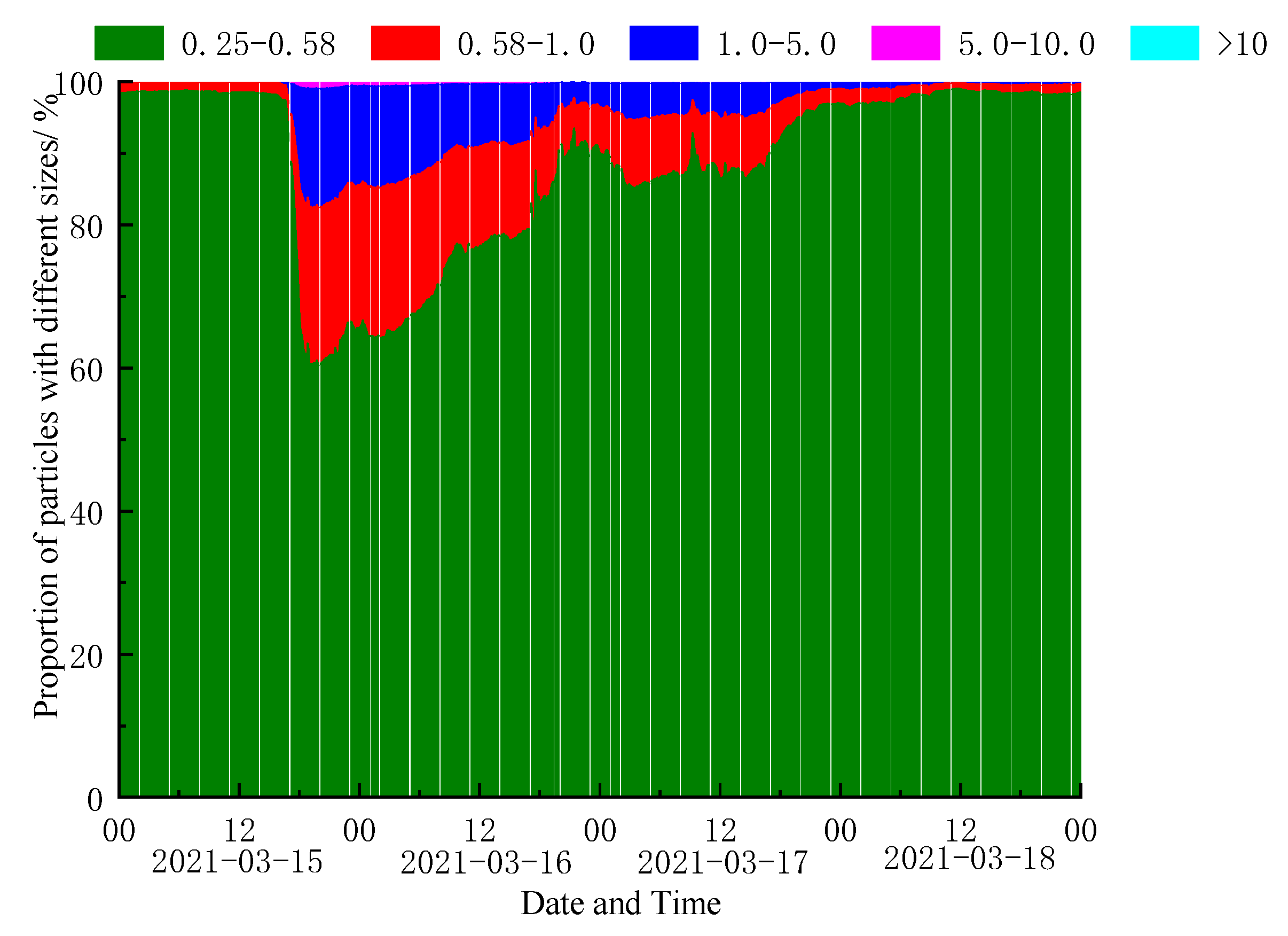
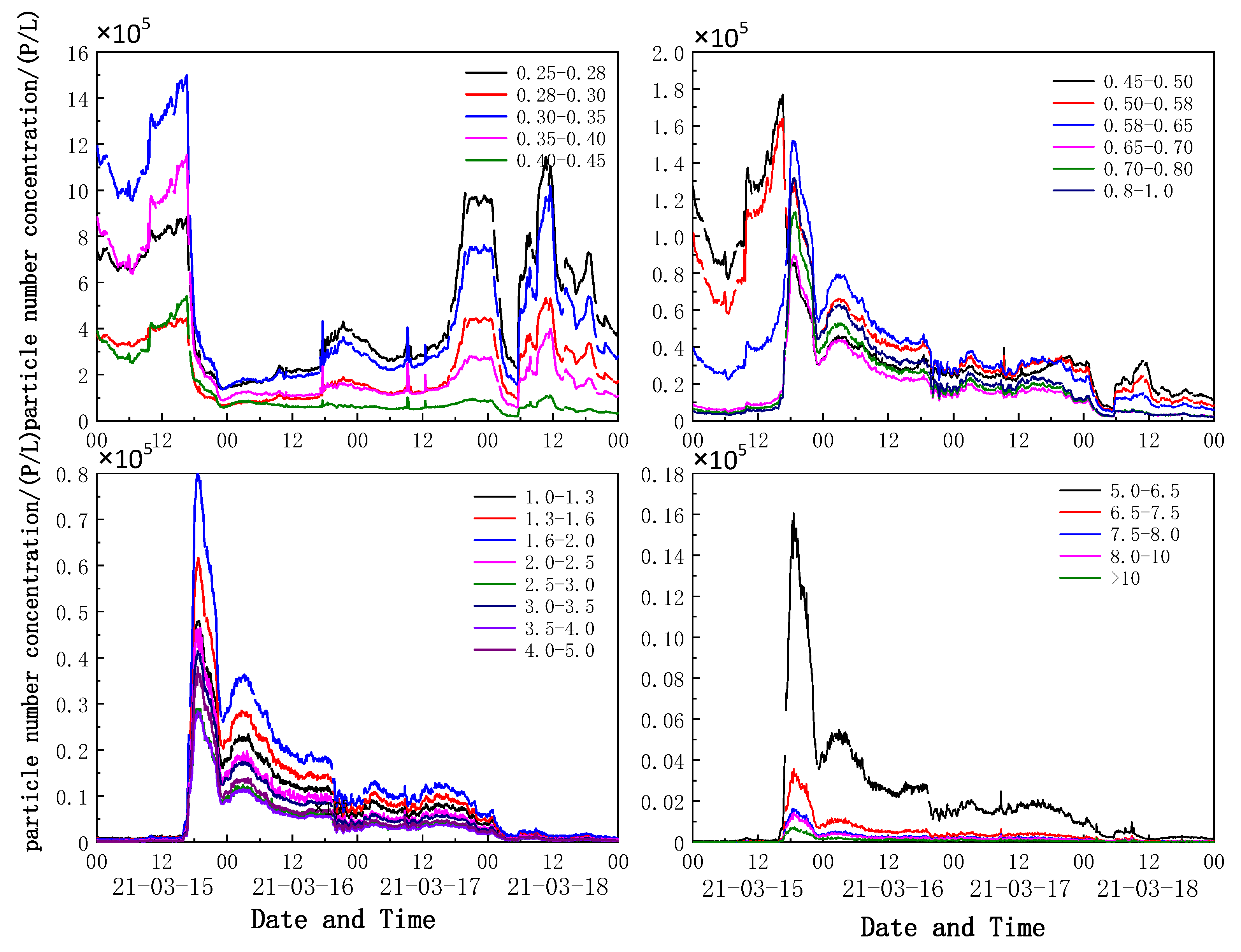
3.4.1. Characteristics of Particle Concentration and Size Distribution

The mass concentrations of PM2.5 and PM10 are shown in Figure 9 (the upper). It was found that the mass concentration of PM1 remained steady throughout the weather process, while the value of PM2.5 and PM10 increased sharply at the arrival of the dust. The change trend of PM2.5 was in good agreement with that of PM10, but the increasing extent of PM10 was much greater than PM2.5. The mass concentration of PM2.5 and PM10 both reached a high value at 18:00 on 15th; their peaks were 573 µg/m3 and 3406 µg/m3, respectively. The mass concentration ratio of PM2.5 to PM10 is shown in Figure 9 (the lower). It is clear from the figure that the value of PM2.5/PM10 collapsed with the sudden increase in PM10. The ratio decreased from 82% at 14:00 to 17% at 18:00 on March 15th. The decline extent was as high as 65%. It is quite evident that the air quality was mainly affected by large particles during dust weather.
Figure 10 describes the size distribution of aerosols observed by EDM180 from 15th to 18th of March. As can be seen from the figure: (1) there were mainly 0.25–0.35 micros particles in the air. (2) From 16:00 to 18:00 on the 15th, the number of particles larger than 0.58 micros (herein referred to as coarse particles) increased rapidly, while the number of particles between 0.25 and 0.58 micros (herein referred to as fine particles) decreased significantly. (3) The moment that the fine particles decreased and the coarse particles increased marked the beginning of the influence of dust. (4) Although the number of particles larger than 6.5 microns also increased when the dust came, the absolute number was small. This also reveals that the particle size of the dust was mainly distributed between 0.58–6.5 microns. (5) The number of fine particles increased dramatically at about 18:00 on the 17th, and the number of coarse particles also showed a small peak at about 15:00. This is due to the returning dust also bringing urban aerosol pollutants, and the deposition of dust particles was earlier than that of the urban aerosol particles. (6) It is also worth noting that the number concentration distribution of coarse particles was consistent with the mass concentration distribution characteristics of PM10, indicating that the mass of particles is mainly contributed by coarse particles.
In order to further expose the change of particle size characteristics during the dust process, the particles were divided into five intervals according to the size, and the number and proportion of particles in each size interval are shown in Table 2 and Figure 11. When dust arrived, the number and particle proportion both increased, except for particles between 0.25–0.58 micros. The proportion of particles between 0.25–0.58 micros decreased from 98% to 60%, while the proportion of particles between 0.58–1.0 micros increased from 1.5% to 22% and the proportion of particles between 1.0–5.0 micros increased from 0.1% to 16%. The proportion of particles between 0.58–5.0 micros increased most significantly. We can see that long-term suspended particles (less than 20 µm) [52] were still dominant during the dust process. It is shown that the dust was mainly long-distance transported dust.

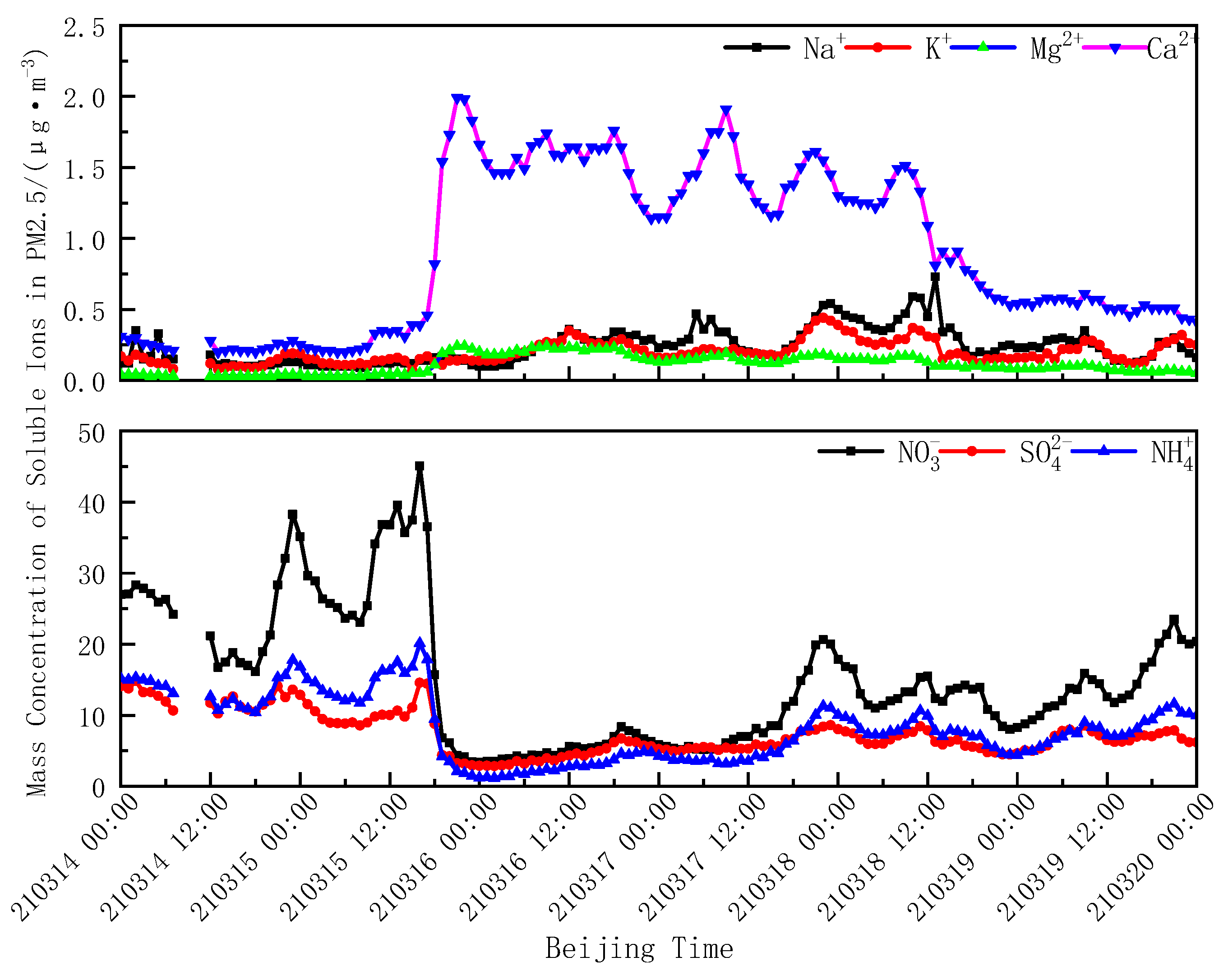
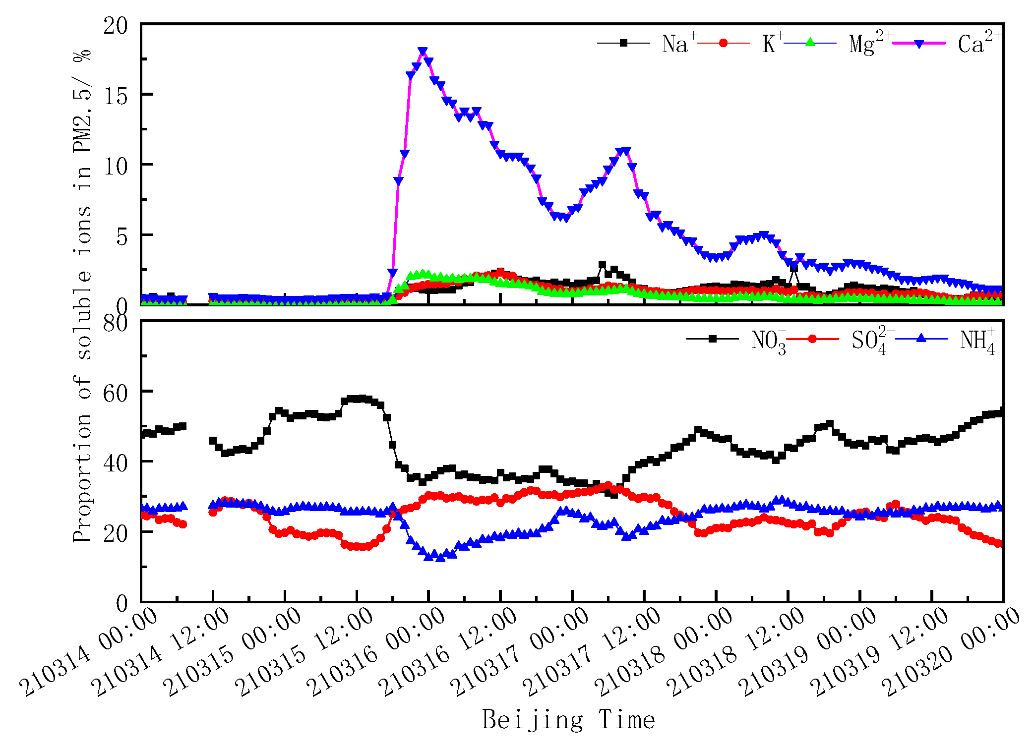
3.4.2. Characteristics of Water-Soluble Particles in PM2.5

Water-soluble ions are an important component of atmospheric particles, and studying them is of great significance [53]. The pollution type can be identified according to the distribution characteristics of water-soluble ions. For example, the main pollution components are secondary pollution ions NO3, NH4+ and SO42− in haze weather; Ca2+ from soil sources increases significantly in dust weather, while K+ and Cl have the greatest influence when burning straw [54]. Figure 12 provides the mass concentration of water-soluble ions in PM2.5 from 14th to 20th March. We found that the mass concentration of NO3, NH4+ and SO42− decreased significantly, while the value of Ca2+ increased rapidly at about 18:00 on 15 March. This phenomenon implies the arrival of dust. At 15:00 on the 17th, the mass concentration of NO3, NH4+ and SO42− began to rise, indicating haze pollution. However, the value of Ca2+ did not fall, which meant the dust was not over. Both the high values of secondary pollution ions and Ca2+ represent that there was dust pollution mixed with urban aerosol pollution in the atmosphere at this time. These results coincide with the observation of lidar and EDM180.
Figure 13 describes the proportion of water-soluble ions in PM2.5 from March 14th to 20 March. At about 18:00 on 15 March, when the dust arrived, the proportion of Ca2+ rose rapidly from 0.5% to 18%. At about 6:00 on 17 March, when the dust flowed back, the proportion of Ca2+ rose rapidly again, from 6.2% to 11%. The recognition function of Ca2+ in dust pollution was verified again. Another interesting phenomenon is that the proportion of SO42− decreased at about 18:00 on 15 March and increased at about 6:00 on 17 March, while the proportion of NO3 and NH4+ reversed. This indicates that the airstream from the North has a high sulfate content, while the airstream from the South has a high nitrate content.

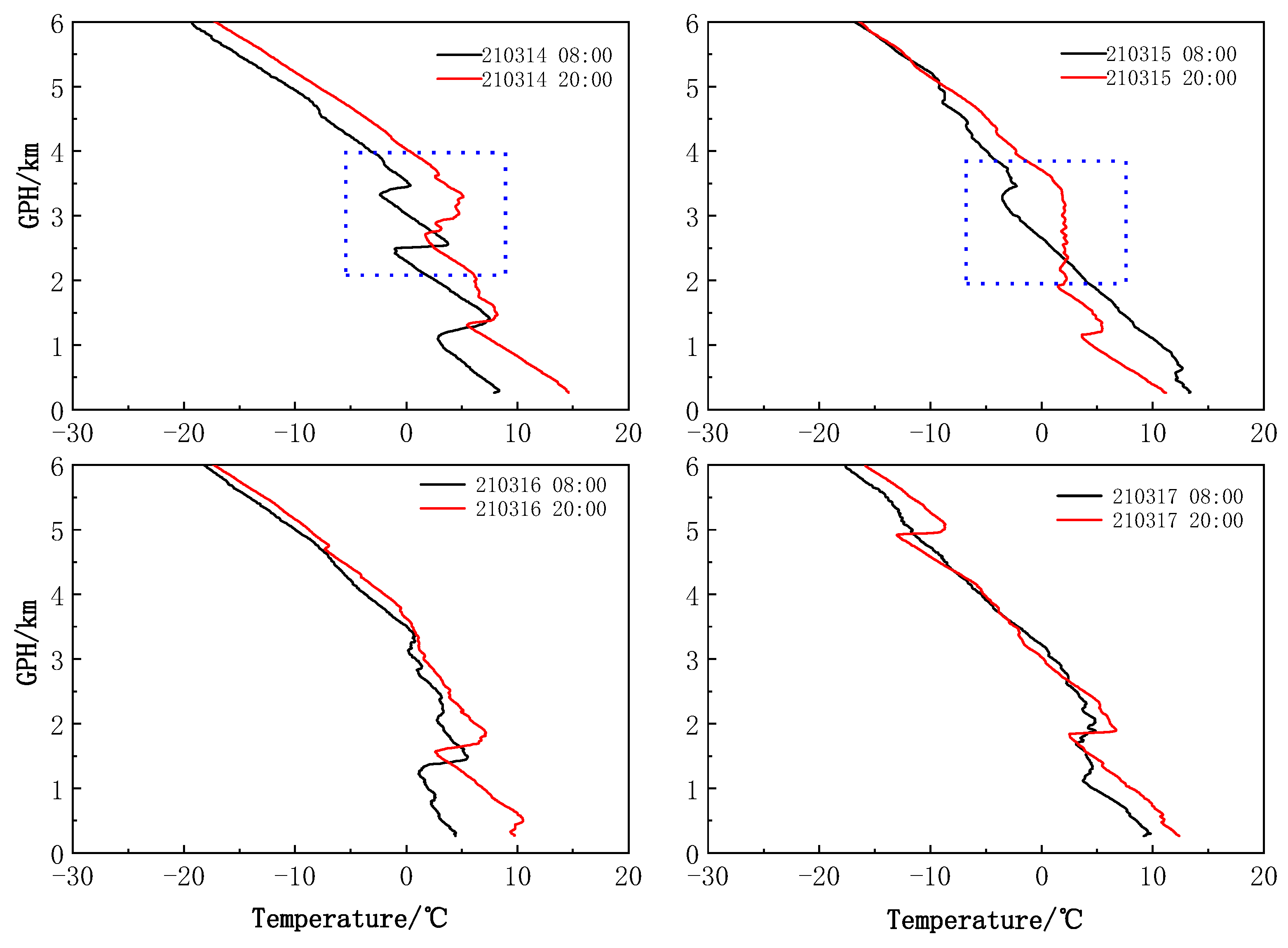
3.4.3. Vertical Structure Characteristics of Temperature

Figure 14 shows the vertical structure of temperature in Jinan from 14–17 March. It is apparent from the graphs that there was a dissimilar inversion layer both at 20:00 on 14th and 15th. The inversion was weak but deep. Such an inversion layer was not observed at 08:00 on the 15th, indicating that dust is more likely to form an inversion layer at night. This also verifies the conclusion that the inversion structure may be related to the radiation effect, in which dust strongly absorbs the surface outgoing infrared radiation at night [2]. As shown in the graphs, there was no similar inversion layer both at 20:00 on the 16th and the 17th. This may be because the dust on the 16th and 17th was weak, and the intensity was insufficient.

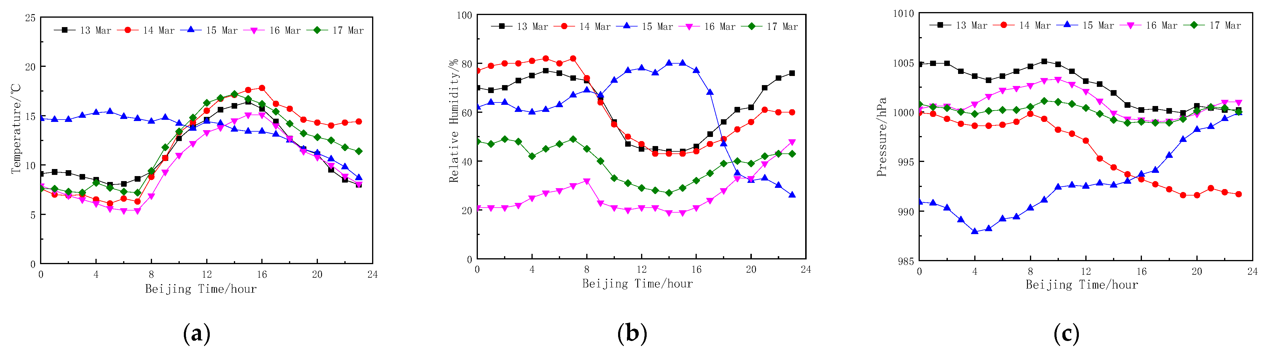
3.4.4. Characteristics of Surface Weather Constituent

Figure 15 describes the changes in temperature, pressure and RH (relative humidity) with time. The data in the figure were measured in a thermometer screen which was 10 m above the ground. According to the curve diagram (a), the pressure began to decrease at 08:00 on the 14th and reached the lowest value of 987.9 hpa at 04:00 on the 15th. Then, the pressure began to rise and returned to the normal level at 23:00 on the 15th. During the whole process, the pressure decreased by 11.9 hpa. According to the curve diagram (b), compared with the normal situation, the temperature decreased less at 19:00 on the 14th. On the 15th, the temperature fixed from 0:00 to 08:00 and a slow decrease began at 08:00. The temperature difference of the whole day on the 15th was 6.7 ℃, which was significantly lower than that of the previous day (11.7 ℃). In general, the RH during the day was lower than that at night. However, according to the curve diagram(c), the RH went up instead of falling at 08:00 on the 15th, and the daytime RH on the 15th was significantly higher than that of other days; Additionally, the RH was dramatically lower on the 16th.
To sum up, pressure decreases in the early stage of dust, while the RH decreases after dust. In the process of dust weather, it becomes cold during the day and warm at night, and the diurnal variation in temperature is inconspicuous.

4. Conclusions

We characterized a strong sandstorm event in China on 15 March 2021 using the synergistic measurements of multi-platform instruments. The main conclusions are as follows:
(1)
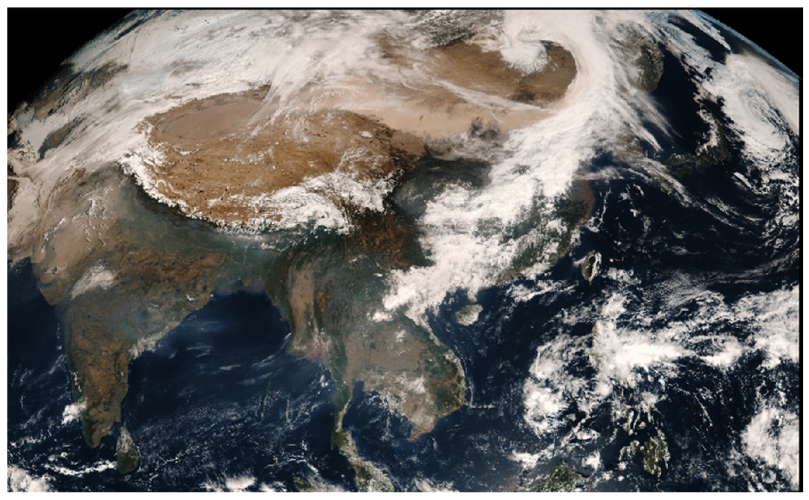
Under the action of the strong Mongolian cyclone, a strong sandstorm occurred in Mongolia on 14 March. Driven by the cold and high pressure after the cyclone, the dust raised by the strong wind moved eastward and southward, affecting most parts of China. The dust arrived in Jinan at 20:00 on 14 March and settled on the ground at 16:00 on 15 March, affecting the local air quality.
(2)
The backward trajectory maps based on HYSPLIT model show that the transport paths of dust changed with time and were not completely identical at different heights. At the beginning, the dust affecting Jinan was from the west and south of Mongolia and the Gobi desert. Then, it came from eastern Mongolia and turned to be flow-back dust brought by the southeast air mass on the 17th.
(3)
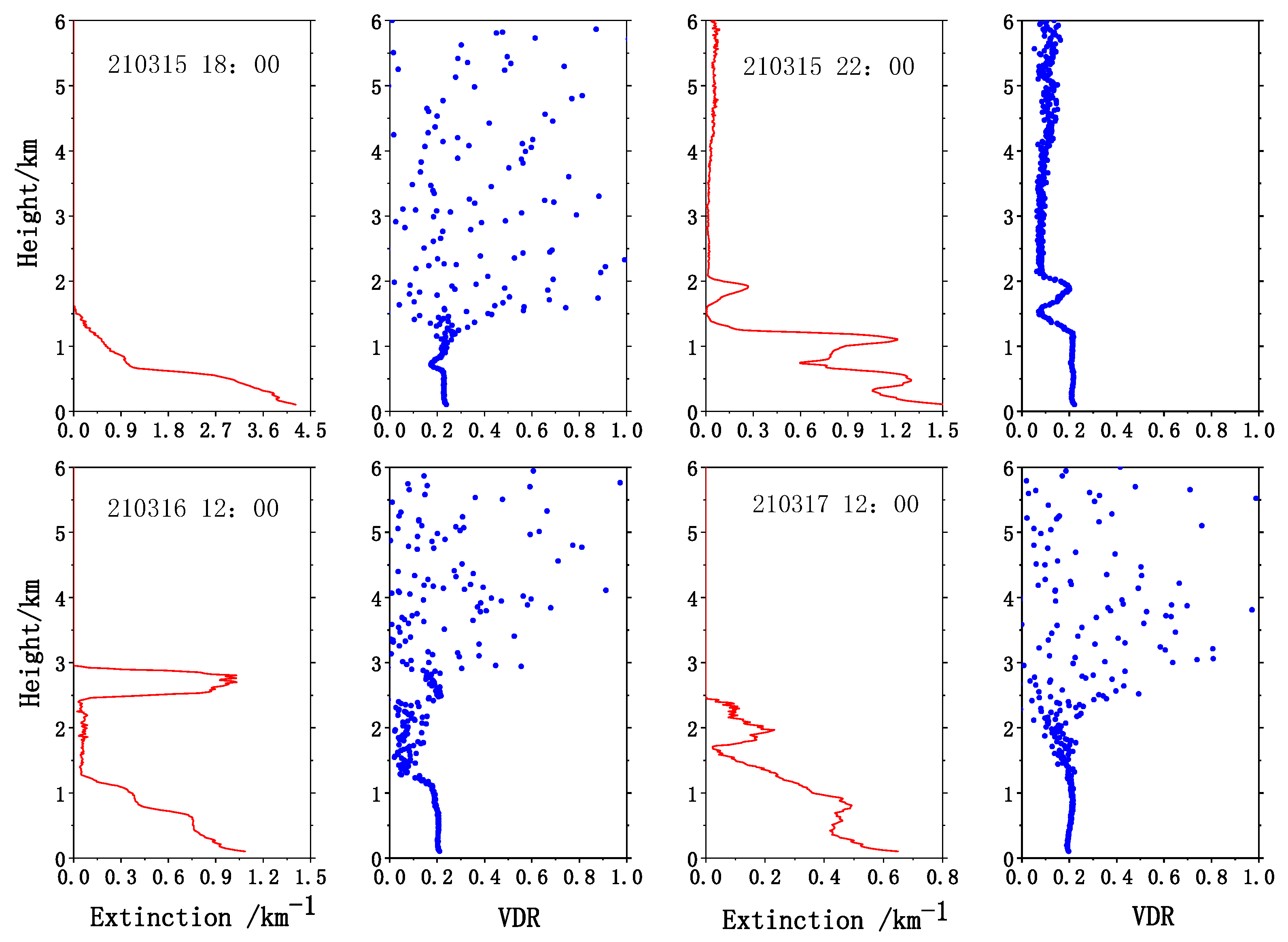
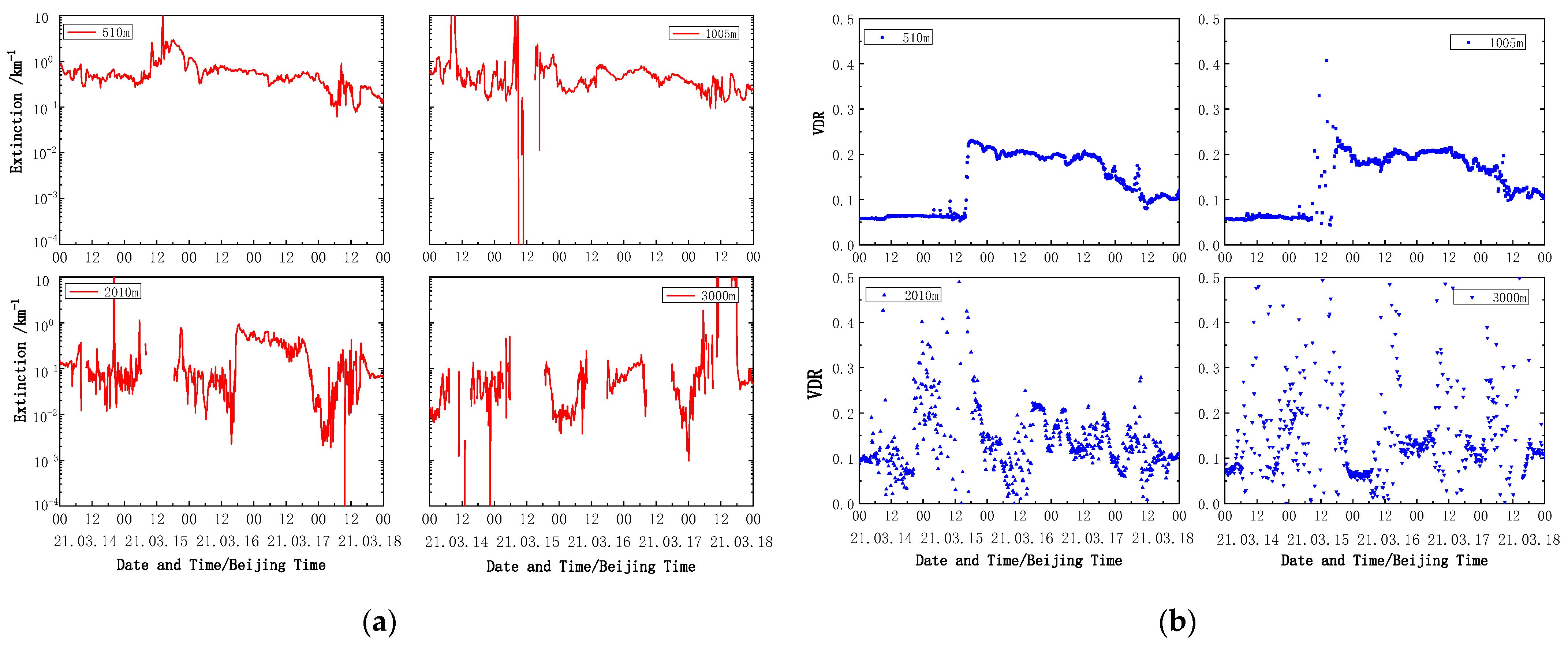
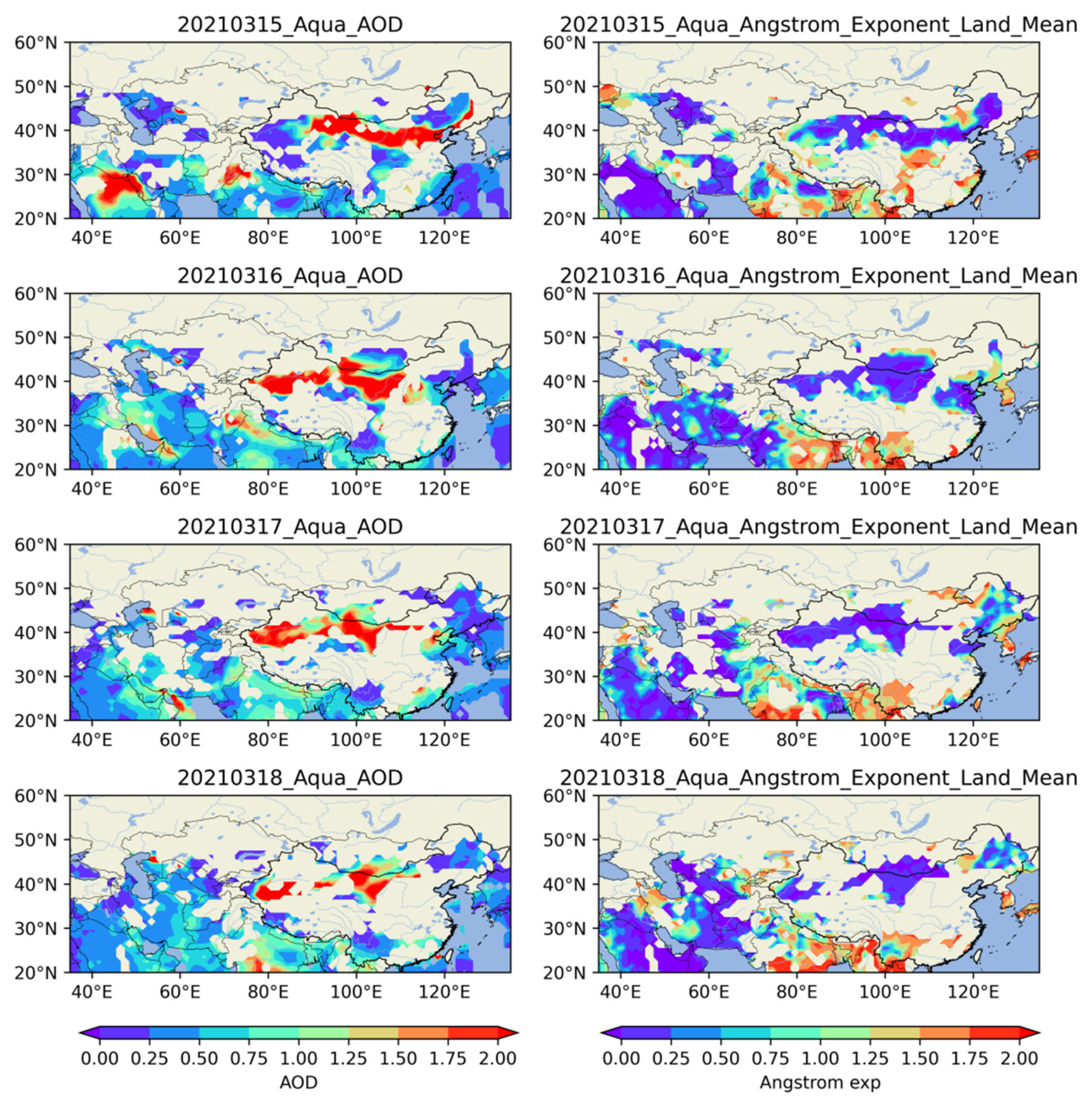
The VDR value of dust observed by lidar was greater than 0.1, mainly around 0.2. The AE value of dust measured by MODIS was less than 0.25. The extinction coefficient observed by lidar and the AOD measured by MODIS are related to dust intensity. The stronger the dust is, the greater the values are. From the lidar observation, found that the higher the transport height was, the smaller the VDR of dust was. This indicates that the sand particles transported in the upper layer were smaller than those in the lower layer.
(4)
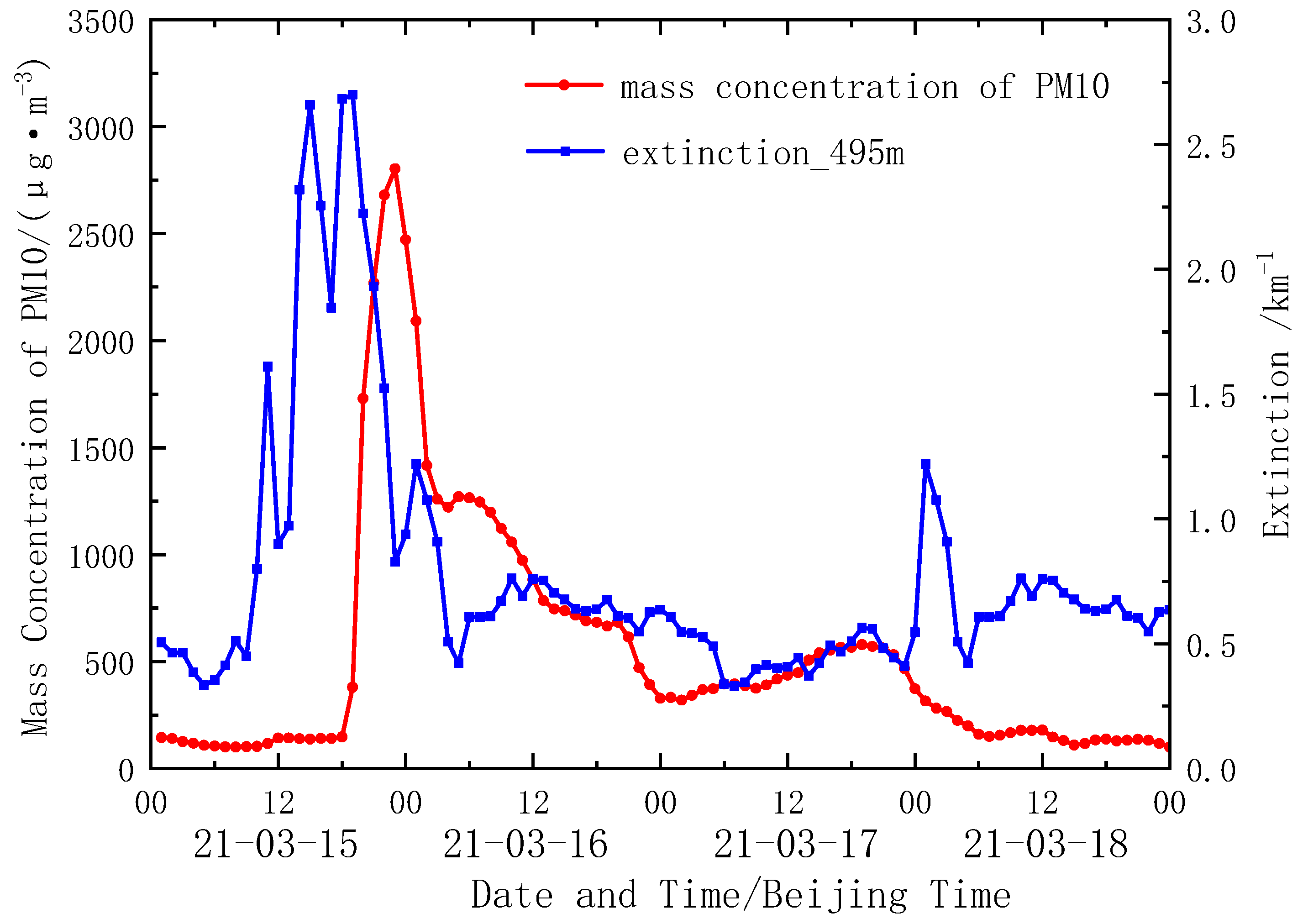
Dust pollution had an obvious impact on the characteristics of particles. In terms of mass concentration, PM1 remained stable, PM2.5 and PM10 increased rapidly, while the ratio of PM2.5 and PM10 decreased steeply. In terms of number concentration, particles between 0.25 and 0.58 micros reduced significantly, while particles larger than 0.58 micros expanded sharply. In terms of water-soluble ionic components, the secondary ion decreased while the calcium ion increased. The peak mass concentrations of PM2.5 and PM10 reached 573 µg/m3 and 3406 µg/m3, respectively. Additionally, the minimum ratio of the two reached 17%. The particle size of the dust was mainly distributed between 0.58–6.50 micros.
(5)
Dust also had an impact on the weather constituent and the vertical structure of air temperature. The pressure decreased in the early stage of dust, while the RH decreased after dust. In the process of dust weather, it becomes cold during the daytime and warm at night, and the diurnal variation of temperature is inconspicuous. A thin and thick inversion layer forms at night because the dust strongly absorbs the surface-outgoing infrared radiation at night.
(6)
Lidar, MODIS, EDM180 and ADI2080 can well identify dust. However, the result of MODIS is affected by observation time and cloud cover. EDM180 and ADI2080 can only capture the dust when it settles on the ground, so the beginning time of dust observed by them is later than that captured by lidar. Although lidar can monitor the vertical stratification and time evolution of dust, it cannot penetrate the polluted layer when the pollution is serious. So, through the combination of multi-platform instruments, the dust process, characteristics and its effects can be better described.

Author Contributions

Conceptualization, A.T., Z.W. (Zhenzhu Wang) and D.L.; methodology, A.T. and Z.W. (Zhenzhu Wang); software, A.T.; validation, Z.W. (Zhifei Wang), J.L. and Y.Z.; formal analysis, A.T.; investigation, Z.W. (Zhenzhu Wang); resources, Z.W. (Zhifei Wang), W.Z. and C.L.; data curation, A.T., Z.W. (Zhenzhu Wang) and X.Z.; writing—original draft preparation, A.T.; writing—review and editing, A.T. and Z.W. (Zhenzhu Wang); visualization, A.T. and X.Z.; supervision, N.W.; project administration, D.L.; funding acquisition, Z.W. (Zhenzhu Wang) and D.L. All authors have read and agreed to the published version of the manuscript.

Funding

This research was funded by National Natural Science Foundation of China, grant number 41975038, and 42111530028; Additionally, funded by Natural Science Foundation of Anhui Province, grant number 2008085J33; Additionally, funded by Key research and Development Program of Anhui Province, grant number 2022h11020008; Additionally, also funded by Youth Innovation Promotion Association CAS, grant number Y2021113.

Data Availability Statement

Data underlying the results presented in this paper are available by contacting the first author or the corresponding author.

Acknowledgments

The authors thank the Natural Science Foundation of China, the Natural Science Foundation of Anhui Province and Chinese Academy of Sciences for help supporting this work. The authors gratefully acknowledge NASA for providing MODIS data and the NOAA Air Resources Laboratory (ARL) for the provision of the HYSPLIT transport and dispersion model and READY website (https://www.ready.noaa.gov accessed on 15 March 2021) used in this publication. The authors also thank all reviewers and editors.

Conflicts of Interest

The authors declare no conflict of interest.

References

  1. Mohammadpour, K.; Sciortino, M.; Kaskaoutis, D.G.; Rashki, A. Classification of synoptic weather clusters associated with dust accumulation over southeastern areas of the Caspian Sea (Northeast Iran and Karakum desert). Aeolian Res. 2022, 54, 100771. [Google Scholar] [CrossRef]
  2. Choobari, O.A.; Zawar-Reza, P.; Sturman, A. The global distribution of mineral dust and its impacts on the climate system: A review. Atmos. Res. 2014, 138, 152–165. [Google Scholar] [CrossRef]
  3. Zender, C.S.; Miller, R.L.; Tegen, I. Quantifying mineral dust mass budgets: Terminology, constraints, and current estimates. Eos Trans. Am. Geophys. Union 2004, 85, 509–512. [Google Scholar] [CrossRef]
  4. Textor, C.; Schulz, M.; Guibert, S.; Kinne, S.; Balkanski, Y.; Bauer, S.; Berntsen, T.; Berglen, T.; Boucher, O.; Chin, M.; et al. Analysis and quantification of the diversities of aerosol life cycles within AeroCom. Atmos. Chem. Phys. 2006, 5, 8331–8420. [Google Scholar] [CrossRef] [Green Version]
  5. Zhao, S.P.; Yin, D.Y.; Qu, J.J. Identifying sources of dust based on CALIPSO, MODIS satellite data and backward trajectory model. Atmos. Pollut. Res. 2015, 6, 36–44. [Google Scholar] [CrossRef] [Green Version]
  6. Huo, W.; Song, M.; Wu, Y.; Zhi, X.; Yang, F.; Ma, M.; Zhou, C.; Yang, X.; Mamtimin, A.; He, Q. Relationships between near-surface horizontal dust fluxes and dust depositions at the centre and edge of the Taklamakan Desert. Land 2022, 11, 959. [Google Scholar] [CrossRef]
  7. Liu, J.; Zheng, Y.; Li, Z.; Flynn, C.; Welton, E.J.; Cribb, M. Transport, vertical structure and radiative properties of dust events in southeast China determined from ground and space sensors. Atmos. Environ. 2011, 45, 6469–6480. [Google Scholar] [CrossRef]
  8. Nabavi, S.O.; Haimberger, L.; Samimi, C. Climatology of dust distribution over West Asia from homogenized remote sensing data. Aeolian Res. 2016, 21, 93–107. [Google Scholar] [CrossRef] [Green Version]
  9. Jin, Q.; Wei, J.; Lau, W.K.; Pu, B.; Wang, C. Interactions of Asian mineral dust with Indian summer monsoon: Recent advances and challenges. Earth-Sci. Rev. 2021, 215, 103562. [Google Scholar] [CrossRef]
  10. Zhang, W.J.; Li, M.; Lv, B.; Lv, C.; Fu, H.; Jiang, T.; Chen, Y. Lidar detection analysis of a sand-dust process in Jinan. Environ. Monit. China 2019, 35, 165–176. [Google Scholar]
  11. Tang, K.; Huang, Z.; Huang, J.; Maki, T.; Zhang, S.; Shimizu, A.; Ma, X.; Shi, J.; Bi, J.; Zhou, T.; et al. Characterization of atmospheric bioaerosols along the transport pathway of Asian dust during the Dust-Bioaerosol 2016 Campaign. Atmos. Chem. Phys. 2018, 18, 7131–7148. [Google Scholar] [CrossRef] [Green Version]
  12. Honda, A.; Matsuda, Y.; Murayama, R.; Tsuji, K.; Nishikawa, M.; Koike, E.; Yoshida, S.; Ichinose, T.; Takano, H. Effects of Asian sand dust particles on the respiratory and immune system. J. Appl. Toxicol. 2014, 34, 250–257. [Google Scholar] [CrossRef] [PubMed] [Green Version]
  13. Arnold, C. Dust storms and human health: A call for more consistent, higher-quality studies. Environ. Health Perspect. 2020, 128, 114001. [Google Scholar] [CrossRef]
  14. Lee, H.; Kim, H.; Honda, Y.; Lim, Y.H.; Yi, S. Effect of Asian dust storms on daily mortality in seven metropolitan cities of Korea. Atmos. Environ. 2013, 79, 510–517. [Google Scholar] [CrossRef]
  15. Qian, L.; Yang, J.H.; Yang, X.L.; Yang, Y.L. Cause analysis of “2008.5.2” strong sandstorm in the eastern of Hexi corridor. Plateau Meteorol. 2010, 29, 719–725. [Google Scholar]
  16. He, Q.; Xiang, M.; Tang, S.J. Synoptic analyses of two strong sandstorms in the hinterland of Taklimakan desert. J. Desert Res. 1998, 18, 320–327. [Google Scholar]
  17. Shen, H.X.; Li, X.L.; Shi, B.J. Comparison analysis of two dust devil events in Beijing area. Meteorlogical Mon. 2004, 30, 12–16. [Google Scholar]
  18. Guo, X.N.; Wang, Y.; Ma, X.M.; Tan, C.R.; Zhang, X.Y.; Zhang, J.N.; Zhang, H.X.; Chen, J. Analysis of a typical heavy dust pollution weather in semi-arid region: A case study in eastern Qinghai. Acta Sci. Circumstantiae 2021, 41, 343–353. [Google Scholar]
  19. Peng, S.L.; Zhou, S.D.; Wei, K.J.; Shen, A. Causes and characteristics of a dust weather process in the Beijing-Tianjin-Hebei region. Trans. Atmos. Sci. 2019, 42, 926–935. [Google Scholar]
  20. Guo, X.N.; Ma, X.M.; Zhang, Q.M.; Tan, C.R.; Ma, Y.C.; Wang, N.; Wang, Y. Analysis of the transmission characteristics of a heavy dust pollution weather in Qinghai Plateau. Environ. Monit. China 2020, 36, 45–54. [Google Scholar]
  21. Yun, J.B.; Jiang, X.G.; Meng, X.F.; Xue-Hong, W.U.; Ying, C. Comparative analyses on some statistic characteristics between cold front and Mongolia cyclone dust storm processes. Plateau Meteorol. 2013, 32, 423–434. [Google Scholar]
  22. Wang, T.H.; Sun, M.X.; Huang, J.P. Research review on dust and pollution using space-borne lidar in China. Trans. Atmos. Sci. 2020, 43, 144–158. [Google Scholar]
  23. Liu, T.H.; Tsai, F.; Hsu, S.C.; Hsu, C.W.; Shiu, C.J.; Chen, W.N.; Tu, J.Y. South-eastward transport of Asian dust:source, transport and its contributions to Taiwan. Atmos. Environ. 2009, 43, 458–467. [Google Scholar] [CrossRef]
  24. Liu, D.; Wang, Z.; Liu, Z.; Winker, D.; Trepte, C. A height resolved global view of dust aerosols from the first year CALIPSO lidar measurements. J. Geophys. Res. Atmos. 2008, 113, D16214. [Google Scholar] [CrossRef]
  25. Qi, Y.L.; Ge, J.M.; Huang, J.P. Spatial and temporal distribution of MODIS and MISR aerosol optical depth over northern China and comparison with AERONET. Chin. Sci. Bull. 2013, 58, 2497–2506. [Google Scholar] [CrossRef] [Green Version]
  26. Eguchi, K.; Uno, I.; Yumimoto, K.; Takemura, T.; Shimizu, A.; Sugimoto, N.; Liu, Z. Trans-pacific dust transport: Integrated analysis of NASA/CALIPSO and a global aerosol transport model. Atmos. Chem. Phys. 2009, 9, 3137–3145. [Google Scholar] [CrossRef] [Green Version]
  27. Cao, X.J.; Zhang, L.; Zhou, B.; Bao, J.; Shi, J.S.; Bi, J.R. Lidar measurement of dust aerosol radiative property over Lanzhou. Plateau Meteorol. 2009, 28, 426–433. [Google Scholar]
  28. Bao, X.R.; Wang, L.N.; Yang, Y.P.; Tao, H.J.; Yang, L.L. Analysis of strong dust process in Lanzhou city: Based on Lidar. J. Arid. Land Resour. Environ. 2021, 35, 92–99. [Google Scholar]
  29. Huang, T.; Song, Y.; Hu, W.D. Lidar detection of a sand-dust process in Dalian, Liaoning, China. J. Desert Res. 2010, 30, 983–988. [Google Scholar]
  30. Deng, M.; Zhang, J.H.; Jiang, Y.L. Vertical distribution and source analysis of dust aerosol in Beijing under the influence of a dust storm. J. Meteorol. Sci. 2015, 35, 550–557. [Google Scholar]
  31. Liu, D.; Qi, F.D.; Jin, C.J.; Yue, G.; Zhou, J. Polarization lidar observations of cirrus clouds and Asian dust aerosols over Hefei. Chin. J. Atmos. Sci. 2003, 27, 1093–1100. [Google Scholar]
  32. Guo, B.J.; Liu, L.; Huang, D.P.; Wang, L.L.; Li, X.L. Analysis of lidar measurements from a dust event. Meteorol. Mon. 2008, 34, 52–57. [Google Scholar]
  33. Dong, X.H.; Nobuo, S.; Bai, X.C.; Qi, H.; Ren, L.J.; Wang, Y.P.; Di, Y.A.; Chen, Y.; Zhao, S.L.; Itiro, M. Application of lidar in sand storm observation—Analysis of dust events of Beijing and Hohhot in spring of 2004. J. Desert Res. 2006, 26, 942–947. [Google Scholar]
  34. Xia, J.R.; Wang, P.C.; Zong, X.M.; Chen, H.B.; Min, M. Stereo monitoring of a dust case using lidar and sun photometer. Environ. Monit. China 2011, 27, 74–81. [Google Scholar]
  35. Xu, D. Development of a Dust-Sand Storms Monitoring System Based on the Sun Photometer with a Preliminary Study on the Observation Precision Influence by Cloud. Master’s Thesis, Nanjing University of Information Science and Technology, Nanjing, China, 2008; pp. 9–18. [Google Scholar]
  36. Yuan, T.; Chen, S.; Huang, J.; Zhang, X.; Luo, Y.; Ma, X.; Zhang, G. Sensitivity of simulating a dust storm over Central Asia to different dust schemes using the WRF-Chem model. Atmos. Environ. 2019, 207, 16–29. [Google Scholar] [CrossRef]
  37. Ginoux, P.; Prospero, J.M.; Torres, O.; Chin, M. Long-term simulation of dust distribution with the GOCART model: Correlation with the North Atlantic Oscillation. Environ. Model. Softw. 2004, 19, 113–128. [Google Scholar] [CrossRef]
  38. Uno, I.; Wang, Z.; Chiba, M.; Chun, Y.S.; Gong, S.L.; Hara, Y.; Jung, E.; Lee, S.-S.; Liu, M.; Mikami, M.; et al. Dust model intercomparison (DMIP) study over Asia: Overview. J. Geophys. Res. 2006, 111, D12213. [Google Scholar] [CrossRef] [Green Version]
  39. Zender, C.S.; Bian, H.S.; Newman, D. The mineral dust entrainment and deposition (DEAD) model: Description and 1990s dust climatology. J. Geophys. Res. 2003, 108, 4416. [Google Scholar] [CrossRef] [Green Version]
  40. Luo, C.; Mahowald, N.M.; Corral, J. Sensitivity study of meteorological parameters on mineral aerosol mobilization, transport, and distribution. J. Geophys. Res. 2003, 108, 4447. [Google Scholar] [CrossRef] [Green Version]
  41. Han, Y.; Wu, Y.; Wang, T.; Xie, C.; Zhao, K.; Zhuang, B.; Li, S. Characterizing a persistent Asian dust transport event: Optical properties and impact on air quality through the ground-based and satellite measurements over Nanjing, China. Atmos. Environ. 2015, 115, 304–316. [Google Scholar] [CrossRef]
  42. Yoon, J.E.; Lim, J.H.; Shim, J.M.; Kwon, J.I.; Kim, I.N. Spring 2018 Asian dust events: Sources, transportation, and potential biogeochemical implications. Atmosphere 2019, 10, 276. [Google Scholar] [CrossRef] [Green Version]
  43. Huang, Y.; Chen, B.; Dong, L.; Zhang, Z. Analysis of a dust weather process over east Asia in May 2019 based on satellite and ground-based lidar. Chin. J. Atmos. Sci. 2021, 45, 524–538. (In Chinese) [Google Scholar]
  44. Shi, Z.L.; Zhang, X.B.; Zhang, R.C. Use of radionuclides to trace sand and dust sources of the March 15, 2021 dust storm event. J. Desert Res. 2022, 42, 1–5. [Google Scholar]
  45. Yang, X.J.; Zhang, Q.; Ye, P.L.; Qin, H.; Xu, L.; Ma, L.; Gong, C. Characteristics and causes of persistent sand-dust weather in mid-March 2021 over Northern China. J. Desert Res. 2021, 41, 245–255. [Google Scholar]
  46. Liang, P.; Chen, B.; Yang, X.P.; Liu, Q.; Zhang, D. Revealing the dust transport processes of the 2021 mega dust storm event in northern China. Sci. Bull. 2022, 67, 21–24. [Google Scholar] [CrossRef]
  47. Tian, X.M.; Liu, D.; Fu, S.L.; Wu, D.C.; Wang, B.X.; Wang, Z.; Wang, Y. Characterization of spring air pollution of Beijing in 2019 using active and passive remote sensing instrument. Int. Arch. Photogramm. Remote Sens. Spat. Inf. Sci. 2019, 42, 153–158. [Google Scholar] [CrossRef] [Green Version]
  48. Levy, R.; Hsu, C.; Sayer, A. MODIS Atmosphere L2 Aerosol Product. NASA MODIS Adaptive Processing System. Goddard Space Flight Cent. USA 2015. [Google Scholar] [CrossRef]
  49. Stein, A.F.; Draxler, R.R.; Rolph, G.D.; Stunder, B.J.B.; Cohen, M.D.; Ngan, F. NOAA’s HYSPLIT atmospheric transport and dispersion modeling system. Bull. Amer. Meteor. Soc. 2015, 96, 2059–2077. [Google Scholar] [CrossRef]
  50. Rolph, G.; Stein, A.; Stunder, B. Real-time Environmental Applications and Display System: Ready. Environ. Model. Softw. 2017, 95, 210–228. [Google Scholar] [CrossRef]
  51. Draxler, R.; Hess, G.D. An overview of HYSPLIT_4 modeling system for trajectories, dispersion and deposition. Aust. Meteorol. Mag. 1998, 47, 295–308. [Google Scholar]
  52. Al-Dousari, A.; Doronzo, D.; Ahmed, M. Types, indications and impact evaluation of sand and dust storms trajectories in the Arabian Gulf. Sustainability 2017, 9, 1526. [Google Scholar] [CrossRef] [Green Version]
  53. Cao, S.; Wu, D.; Chen, L.Z.; Xia, J.R.; Lu, J.G.; Liu, G.; Li, F.Y.; Yang, M. Pollution characteristics of water-soluble ions in atmospheric aerosols in China. Environ. Sci. Technol. 2016, 8, 103–115. [Google Scholar]
  54. Han, Y.M.; Shen, Z.X.; Cao, J.J.; Li, X.-X.; Zhao, J.-L.; Liu, P.P.; Wang, Y.H.; Zhou, J. Seasonal variations of water-soluble inorganic ions in atmospheric particles over Xi’an. Environ. Chem. 2009, 28, 261–266. [Google Scholar]
Figure 1. Mongolian cyclone observed by FY-4A on 15 March 2021.
Remotesensing 14 03593 g001
Figure 2. Weather situation map (a) 500 hPa, (b) 850 hPa, (c) surface at 08:00 on 15 March and (d) time evolution of three-dimensional wind (color, unit Pa·s−1).
Remotesensing 14 03593 g002
Figure 3. Extinction coefficient (ae) and VDR (fj) from 14 March to 18 March.
Remotesensing 14 03593 g003
Figure 4. Vertical profiles of the extinction coefficient (read lines) and the VDR (blue lines) at several typical moments.
Remotesensing 14 03593 g004
Figure 5. Time distribution of the extinction coefficient (a) and the VDR (b) at several typical heights.
Remotesensing 14 03593 g005
Figure 6. Time distribution of the extinction coefficient at 495 m and the mass concentration of PM10 on the surface.
Remotesensing 14 03593 g006
Figure 7. The map of 48 h backward trajectories, the (ad) sub-graphs represent the trajectories with the start time at 18:00 of 15 March, 22:00 of 15 March, 12:00 of 16 March and 12:00 of 17 March, respectively.
Remotesensing 14 03593 g007
Figure 8. The evolution of Aqua-MODIS AOD and AE from 15 March to 18 March.
Remotesensing 14 03593 g008
Figure 9. Mass concentration of PM1, PM2.5 and PM10 (the upper), and mass concentration ratio of PM2.5 to PM10 (the lower).
Remotesensing 14 03593 g009
Figure 10. Number concentration of different particle size varying with time.
Remotesensing 14 03593 g010
Figure 11. Particle proportion of different size intervals, varying with time.
Remotesensing 14 03593 g011
Figure 12. Mass concentration of water-soluble ions in PM2.5.
Remotesensing 14 03593 g012
Figure 13. Proportion of water-soluble ions in PM2.5.
Remotesensing 14 03593 g013
Figure 14. Vertical profile of the atmospheric temperature, the longitudinal coordinate of the figure is the GPH (geopotential height).
Remotesensing 14 03593 g014
Figure 15. Variation curve of surface weather constituent (ac) with time.
Remotesensing 14 03593 g015
Table 1. The 31 particle channels of EDM180, N represents the channel order and D represents the channel diameter in the unit of microns.
NDNDNDNDND
1>0.258>0.5815>2.022>7.529>25.0
2>0.289>0.6516>2.523>8.030>30.0
3>0.3010>0.7017>3.024>10.031>32.0
4>0.3511>0.8018>3.525>12.5
5>0.4012>1.019>4.026>15.0
6>0.4513>1.320>5.027>17.5
7>0.5014>1.621>6.528>20.0
Table 2. Number of particles in each size interval during the dust process.
Date0.25–0.58 µm0.58–1.0 µm1.0–5.0 µm5.0–10.0 µm>10.0 µmAll
03–149.42 × 1088.99 × 1066.88 × 1052.87 × 1042.56 × 1039.52 × 108
03–158.14 × 1083.70 × 1072.02 × 1071.12 × 1063.57 × 1048.73 × 108
03–162.28 × 1084.03 × 1072.56 × 1071.12 × 1063.08 × 1042.95 × 108
03–173.60 × 1082.23 × 1071.23 × 1076.13 × 1051.93 × 1043.95 × 108
03–184.55 × 1086.06 × 1062.33 × 1061.36 × 1056.77 × 1034.63 × 108
Publisher’s Note: MDPI stays neutral with regard to jurisdictional claims in published maps and institutional affiliations.

