Abstract
In this study, we present a nationwide machine learning model for hourly PM estimation for the continental United States (US) using high temporal resolution Geostationary Operational Environmental Satellites (GOES-16) Aerosol Optical Depth (AOD) data, meteorological variables from the European Center for Medium Range Weather Forecasting (ECMWF) and ancillary data collected between May 2017 and December 2020. A model sensitivity analysis was conducted on predictor variables to determine the optimal model. It turns out that GOES16 AOD, variables from ECMWF, and ancillary data are effective variables in PM estimation and historical reconstruction, which achieves an average mean absolute error (MAE) of 3.0 g/m, and a root mean square error (RMSE) of 5.8 g/m. This study also found that the model performance as well as the site measured PM concentrations demonstrate strong spatial and temporal patterns. Specifically, in the temporal scale, the model performed best between 8:00 p.m. and 11:00 p.m. (UTC TIME) and had the highest coefficient of determination (R) in Autumn and the lowest MAE and RMSE in Spring. In the spatial scale, the analysis results based on ancillary data show that the R scores correlate positively with the mean measured PM concentration at monitoring sites. Mean measured PM concentrations are positively correlated with population density and negatively correlated with elevation. Water, forests, and wetlands are associated with low PM concentrations, whereas developed, cultivated crops, shrubs, and grass are associated with high PM concentrations. In addition, the reconstructed PM surfaces serve as an important data source for pollution event tracking and PM analysis. For this purpose, from May 2017 to December 2020, hourly PM estimates were made for 10 km by 10 km and the PM estimates from August through November 2020 during the period of California Santa Clara Unite (SCU) Lightning Complex fires are presented. Based on the quantitative and visualization results, this study reveals that a number of large wildfires in California had a profound impact on the value and spatial-temporal distributions of PM concentrations.
1. Introduction
Aerosols are collections of solid or liquid particles suspended in the air [1]. Generally, aerosol refers to airborne particulate materials that originate from a variety of sources, such as fossil fuel, biomass burning, desert dust, and marine [2]. A number of environmental issues are associated with aerosols, including haze, acid rain, and greenhouse effect [3,4,5]. Aerosol particulates vary in size and shape, such as PM (the particle diameter is 2.5 microns or less) and PM (the particle diameter is 10 microns or less). Among these aerosol particulate types, PM raises the most research interest because of its inhabitable fine size. It has been found that PM has a negative impact on human health and are linked to many diseases such as lung cancer, asthma, and cardiovascular diseases [6,7,8,9,10,11]. These diseases can further cause behavioral effects, such as absenteeism and poor performance at school [12,13,14]. Understanding the distribution of PM in a high temporal and spatial resolution is essential to address health concerns.
Aerosol particles are usually too small to be seen by the human eye, but they exist everywhere in the atmosphere with highly varying properties across space and time [1]. Because aerosols are highly inhomogeneous in space and time, continuous observation is essential for a comprehensive study. In situ monitoring networks, such as the United States Environmental Protection Agency (EPA) PM monitoring networks [2,15], which include more than 500 sites across the country, are considered to be the most reliable type of sources providing aerosol information. However, the sparse coverage and unbalanced distribution of these monitoring networks do not provide sufficient data to determine the public’s risk of exposure to PM. Thus, a wide range of studies have been conducted to either improve the scope and accuracy of PM acquisitions, or model and estimate PM concentrations by considering a variety of variables. The following section summarizes some important trending PM studies.
1.1. An Overview of PM Modeling and Estimation Approaches
Some research focuses on increasing the number of monitoring networks to extend the observation scope by utilizing machine learning [16,17,18]. For example, a machine learning-based calibration method was used for low-cost airborne particulate sensors, which helps to improve the measurement accuracy of cheap sensors and allows these sensors to be a complementary monitoring network for environmental agencies [19]. This research expands the scope of the currently available airborne particulates monitoring networks and allows for a finer resolution on a regional scale.
On the other hand, some studies focus on fusing ground PM measurements and satellite derived products for PM modeling and estimation [20,21,22,23,24,25,26,27,28,29,30]; of these studies, some of the most comprehensive in terms of contextual variables considered were [20,21]. In addition to satellite variables, meteorological variables including relative humidity, planetary boundary layer high, wind and direction, and the vertical aerosol structure distribution are found to be important factors in PM modeling [27,28].
There have been studies that have explored machine learning methods for PM modeling. Tree-based methods, deep networks, and the combination of traditional machine learning methods with ancillary data were found to be effective methods in PM modeling [22,29,31,32,33,34,35]. Statistical methods and physical or chemical theories based methods were also found capable in PM modeling, such as the urban fine scale PM estimation by using Landsat 8 images [36], Gaussian processes modeling in a Bayesian hierarchical setting [10], long-term estimation using remote sensing products and chemical transport models [37], and the estimating of PM using a hybrid method that combines multiple sub-models [38].
These studies have one or more of the following three major limitations. First, the relationship between PM concentrations and remote sensing data was explored at a local scale or under strict assumptions, which is not easily extended to a larger scale. Second, the low temporal resolution remote sensing product is used, which does not allow high temporal PM estimation. Third, many influential factors are not considered, thus limiting the representativeness of the model.
1.2. A Machine Learning Approach Using Data from Geostationary Satellites
Some of the widely used satellite products for PM estimation are summarized in Table 8. Both Moderate Resolution Imaging Spectroradiometer (MODIS) and Visible Infrared Imaging Radiometer Suite (VIIRS) provide high spatial but low temporal resolution Aerosol Optical Depth (AOD) products as a result of their polar orbit characteristics, passing through both poles in one rotation. The time interval between two satellite “brushes” in a specific area causes the PM estimation gaps [28,29]. These temporal gaps pose difficulties for applications and studies that need high temporal PM estimation, such as detecting extreme environmental pollution and human health research. In such circumstances, a geostationary satellite that is on orbit above the equator at a height of 35,786 km and that follows the rotation of the earth would be able to obtain high-resolution spatial and temporal data from the area being observed.
Using the data collected from May 2017 to December 2020, and building on the approach used previously by [20,21], this study develops machine learning models for estimating hourly PM concentrations at a 10 km spatial resolution. European Centre for Medium-Range Weather Forecasts (ECMWF) meteorological parameters, Geostationary Operational Environmental Satellites (GOES-16) AOD products, and ancillary variables are collected for model training. Hourly observations from 586 EPAs collected across the US along with GOES-16 AOD and ancillary variables as predictors allow PM estimations on the continental US with unprecedented temporal resolution. Once the model is established, the performances are evaluated on influential variables. In addition, historical hourly PM surfaces are estimated and the historical surfaces under the influence of wildfires are presented.
The contributions of this study can be summarized in these aspects. First, the GOES-16 continuously monitors the US territory and generates AOD surfaces every five minutes at a native spatial resolution of two kilometers. By contrast to the widely used polar orbit AOD product, such as MODIS, the high temporal resolution of the satellite enables the estimation of PM surfaces covering the U.S. territory in a high temporal resolution. These reconstructed PM surfaces across the country are valuable data sources for monitoring high dynamic pollution events, such as wildfires, and for epidemiological studies in a continuous spatial domain. Challenges still exist because the training and the reconstruction process is extremely computation intensive, in which hundreds of CPUs and multiple TB of memory are required. Hence, the second contribution of the study comes in utilizing multiple high performance computing platforms to make the hourly nationwide PM reconstructions from May 2017 to December 2020. These reconstructed PM surfaces are also delivered in daily and monthly resolutions. The high platforms include the Texas Advanced Computing Center (TACC) and the Texas Research and Educational Cyberinfrastructure Service (TRECIS). Third, data from a wide range of predictor variables are included, including data from ECMWF, location-specific solar angles, elevation, population density, soil type, landcover type, and lithology (see Table 1). These predictors provide a comprehensive description of the environmental and geological variations that are essential to capture the PM variation in time and space, and thus enable a robust estimation model. The model performances are systematically investigated by taking into account the time of day, seasons, elevation, population density, and land cover type in order to gain a more in-depth understanding of PM distribution patterns and their application potential.

Table 1.
The predictor variables used for the nationwide PM study as well as their source and descriptions are listed.
2. Materials and Methods
2.1. Data Sources and Pre-Processing
2.1.1. Nation Level PM Ground Observations
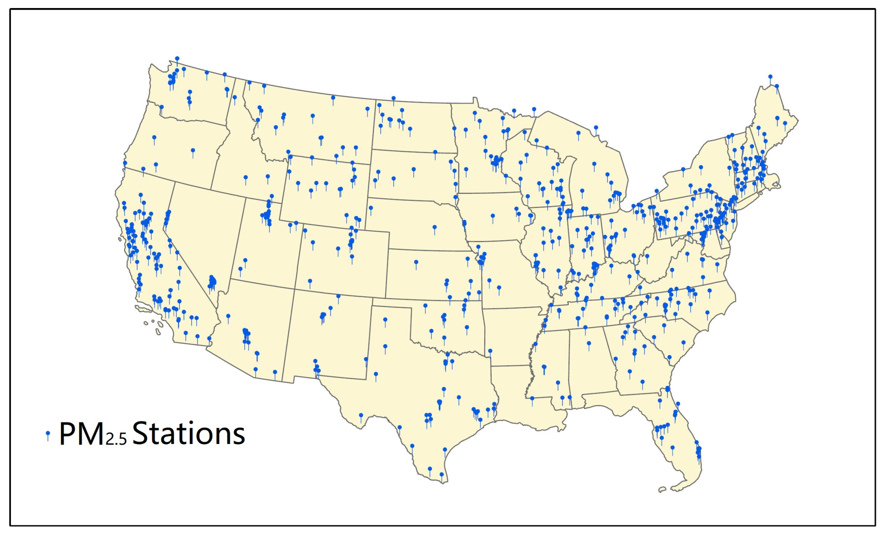
The EPA provides PM ground observations for the past six months through the AirNow API and all other historical PM archive data via the Air Quality System (AQS) API. PM observations are collected at hourly intervals from 685 monitoring (see Figure 1) sites between May 2017 and December 2020 through AQS APIs. The EPA has a long-standing convention of allowing negative data into the AQS. If the atmosphere is very clean and there is noise in the measurement, negative values could be generated due to the equipment error, which are excluded in this research.
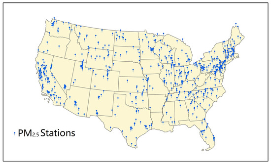
Figure 1.
The map illustrates the 685 PM monitoring sites providing the training data.
2.1.2. ECMWF Grid
The ECMWF climate data store provides hourly ERA5 land reanalysis data from 1979 to present. The gridded EAR5 file comes in the GRIB format with a 0.1× 0.1 horizontal resolution and hourly temporal resolution in global coverage. Historical gridded EAR5 data from May 2017 to December 2020 are collected and matched with the PM grid. A total of eight meteorological parameters have been selected for PM modeling and estimation (see Table 1).
2.1.3. GOES-16
GOES-16 AOD data are available every five minutes in NetCDF format on Amazon S3. The raw data have its own GOES-R ABI fixed grid projection. The projection coordinate system is converted to a geographic coordinate system based on the perspective point height and sweep angle axis information in the metadata before any value can be from the file. AOD’s values are ready to be retrieved after the conversion is complete. The AOD and the Data Quality Flag (DQF) from May 2017 to December 2020 are retrieved from AWS in 2 km spatial resolution and 5 min temporal resolution. For matching purposes, the projection coordinate system is converted from a fixed grid projection to a geographic coordinate system.
2.1.4. Ancillary Data
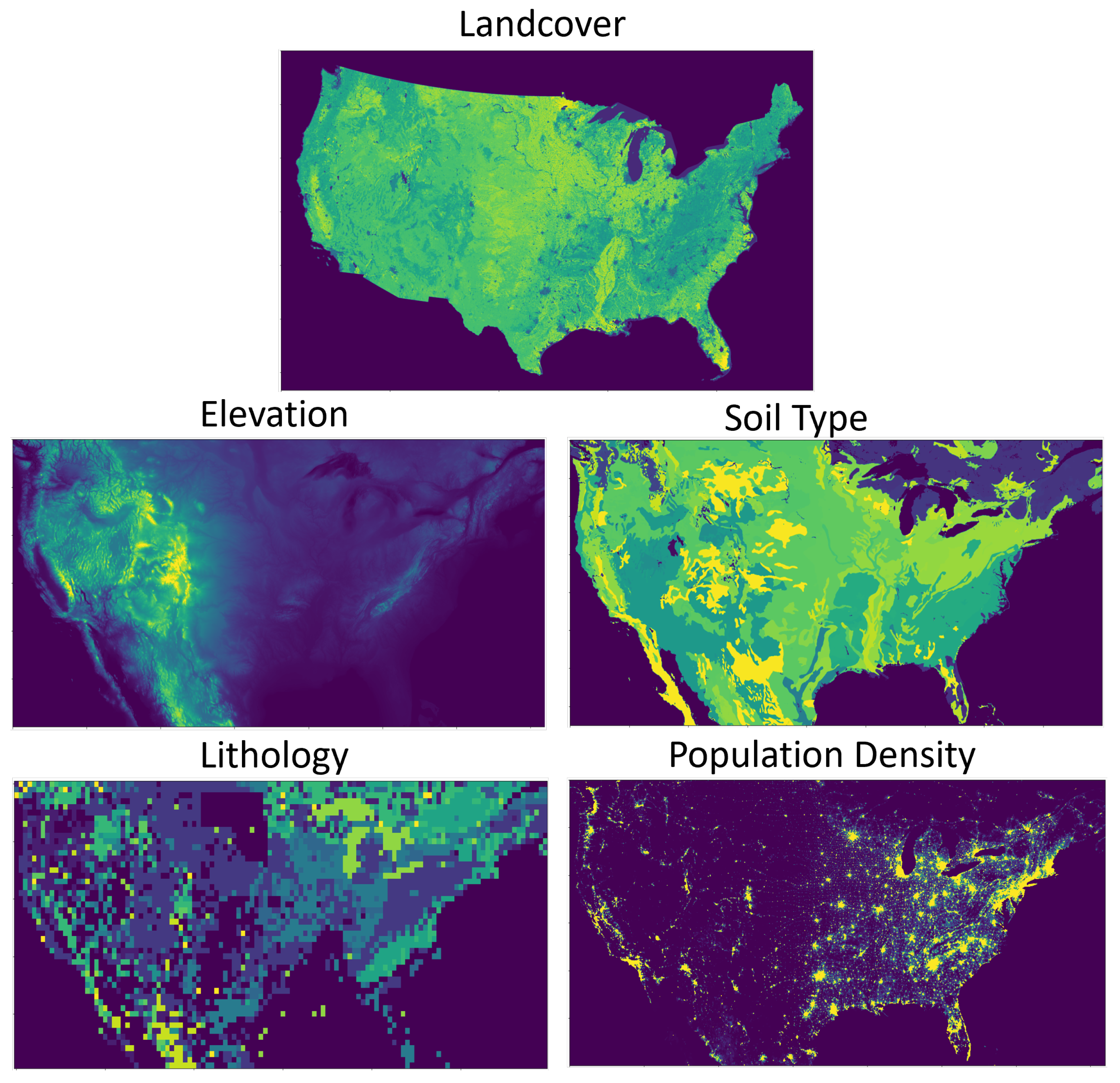
Different types of ancillary data were used in the study, including solar angles, landcover, soil types, lithology types, and Gebco elevations (see sample images in Figure 2). The data were in different spatial extents and projection coordinate formats. Before aligning these ancillary data with the PM values, pre-possessing work is completed, including data cropping and coordinate conversion. The solar azimuth angle and solar zenith angle are calculated according to geographic placement and time.

Figure 2.
The ancillary raster images which include landcover, elevation, soil type, lithology, and population density.
2.2. Data Matching
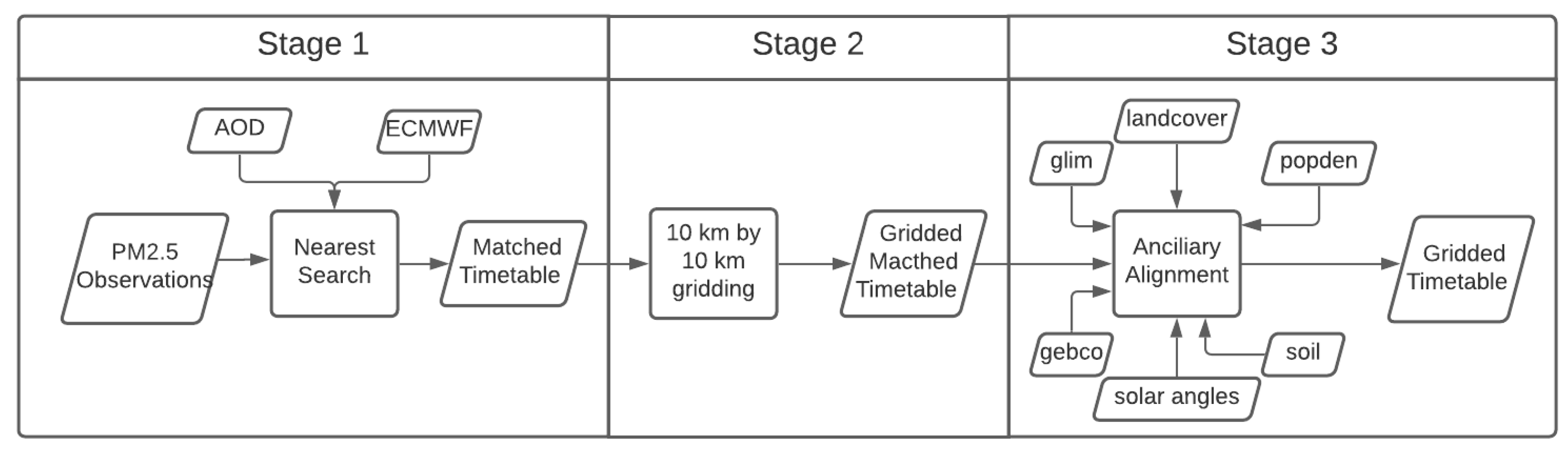
EPA ground observations, ECMWF meteorological data, and AOD from GOES-16 are all collected at different times and in different formats. It is necessary to match up these datasets into a consistent timetable for model training. Figure 3 illustrates the three stages of the data matching process. In stage 1, the coordinates and the time stamp information of each PM ground observation are retrieved, which are used as query parameters to obtain AOD, meteorological parameters from GOES-16 and ECMWF respectively based on the nearest search method. During Stage 2, a grid of 10 × 10 km is generated and overlaid on the matched data, and the values within each grid cell are averaged. In stage 3, the ancillary data including solar zenith angle, solar azimuth angle, population density, landcover, soil type, lithology and elevation information are aligned with each grid cell.
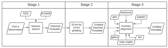
Figure 3.
An overview of the three stages of data matching and gridding.
In stage 1, there are always grid pixels from AOD and ECMWF that do not perfectly match the coordinate and timestamp from the PM observations. In these cases, the nearest search method is used. As a specific example, in the temporal domain, PM observations and the ECMWF are recorded hourly, while the AOD is recorded every five minutes. Consequently, the AOD, a file whose timestamp is closest to the PM observation timestamp, is selected for matching. In the spatial domain, both the AOD and ECMWF surfaces are composed of equal distance grids. Each grid’s coordinates are assigned at its grid center. As a result, a perfect coordinate match between PM and grid files is a rare case. Practically, a nearest search method is adopted to match the values between these data sources by adding a distance tolerance value. Tolerance values are defined as the same as the resolution of target files. Once the matching is complete, a timetable containing PM observation values, meteorological factors, and AOD is generated. The observations with failed matching values are deleted.
2.3. Experiment Design
In order to investigate the effectiveness of selected variables in the PM modeling, four types of models with different predictor variables were developed—the base model, the AOD model, the ancillary model, and the full model. Only ECMWF meteorological variables are used as predictors in the base model. In addition to the ECMWF variables, the AOD model includes the AOD product from GOES-16 as an additional predictor. Rather than the AOD product, variables from ancillary sources are used as predictors in the ancillary model. Finally, all the variables discussed are included in the full model. Once the hyper-parameters have been optimized using the 10-folder cross-validation technique, the best model with its optimized parameters is finalized and validated on the training and test datasets. Then, the performance of the model is examined on a temporal and spatial scale.
A gridded timetable is generated from the three-stage matching process. The timetable includes 1,420,810 entries between May 2017 and December 2020, and includes all the variables that are listed in Table 1. The timetable is divided into training and testing groups with a 90/10 ratio for machine learning model training and testing. Based on the choices of predictors, four types of machine learning models are developed. The hyper-parameter optimization is implemented on the four models based on a 10-fold cross-validation optimization technique. In this process, the training set has been split into 10 groups. Among each unique group, one group is held out and the remaining groups are used as training data. Then, a model is fitted on the training set and is evaluated with the hold out dataset. The performance of the model is summarized after ten iterations. As a result, the best performing predictors and hyper-parameters are utilized to establish a final model on the entire training dataset. Validation of the model is performed on the test dataset once it has been finalized. Validation results, including the Mean Absolute Error (MAE), Root Mean Square Error (RMSE), and the R, are analyzed spatially and temporally. Figure 4 shows the workflow including the process of model training, validation, hyperparameter-optimization, and testing.
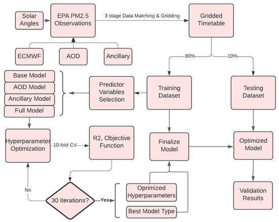
Figure 4.
The flow chart illustrates the process of model training and finalization.
2.4. Machine Learning Approach
In PM modeling and estimation, various approaches have been employed, which can be divided into statistical and machine learning approaches. The statistical approach achieves relatively high model accuracy; however, they have strict assumptions, which limit their applicability. On the other hand, machine learning applications in environmental studies remain an active research topic [39,40], particularly for air pollution issues due to its non-parametric features and efficiency. PM concentration could be affected by a number of factors, including, but not limited to, the variables in Table 1. Its non-parametric nature enables the machine learning approach to be an effective PM study method due to the lack of theories that describe the correlation between variables and PM concentrations. The most common ones are deep neural network, XGBoost, random forest, and neural network. Among these approaches, tree-based approaches including random forest, Boosting tree, and Bagging tree have unique advantages in PM studies in three aspects. In the first place, it provides an explanation of the contribution each predictor variable makes to the model. Secondly, it is faster than other machine learning approaches when dealing with large datasets. Third, the ensemble of weak learners is effective in controlling variance and bias [41]. A total of 1,420,810 observations with 17 predictor variables are used in this study for model training and testing. The 17 predictor variables were collected from different sources with different spatial and temporal resolutions. As a result, noise could get introduced as the data are matched and gridded. Hence, the extra tree regressor (ET), a variation of tree-based ensemble methods based on random forest, is utilized for PM modeling for the three considerations. First, ET has been explored in some regional PM studies [42], and turns out to be an effective method in PM modeling based on AOD and meteorological variables. However, its application potential with various predictors from different sources over the entire US are under explored. Second, ET introduces a greater randomness to the system than random forest, making it more effective at controlling variances and bias, as long as fewer irrelevant predictor variables are included in [43]. Thirdly, ET is faster than random forest by bypassing the optimal split point searching process. Random forest and ET are compared in details below.
2.4.1. Random Forest
A random forest is an ensemble of decision trees. Each tree in a random forest model provides a prediction output independently, and the prediction with the most votes or the average of all predictions is the final prediction output. The advantage of random forest over decision trees is its ability to generate less biased prediction results by aggregating the output from many low-correlated tree models, thereby making tree model errors compensate for each other and contributing to the overall direction of the model [41]. The key to an effective random forest is the low correlation between the tree models. In the case of high correlations, the random forest model would not benefit from the ensemble approach and would produce similar results with individual trees. The Bagging technique (bootstrap aggregation) is used for model training. Instead of dividing the whole training dataset into K chunks in K-cross validation, bagging randomly draws N (the same number as the size of the training dataset) samples from the training dataset with replacement and feeds that N training data to each tree model. Moreover, feature bagging, which is also known as “feature selection”, is also used to generate feature randomness. Usually, features are chosen randomly (from the whole feature pool) for each tree within the random forest model.
2.4.2. Extra Tree
The extra tree and random forest are both ensemble methods of decision trees, but differ mainly in two aspects. On one hand, as an alternative to bootstrapping with replacement in a random forest, extra tree trains each individual tree model using the entire learning sample, helping to reduce bias. On the other hand, unlike a random forest, which selects the optimal local cutting point based on information gain, the extra tree selects the cut-points randomly. Then, out of all these randomly chosen cut-points, the one that yields the most accurate result is chosen as the cut-point of the tree learner. It skips the process of cut-point optimization, which helps to reduce the model variance and speeds up the tree-building process [43].
3. Results
3.1. Model Comparison and Finalization
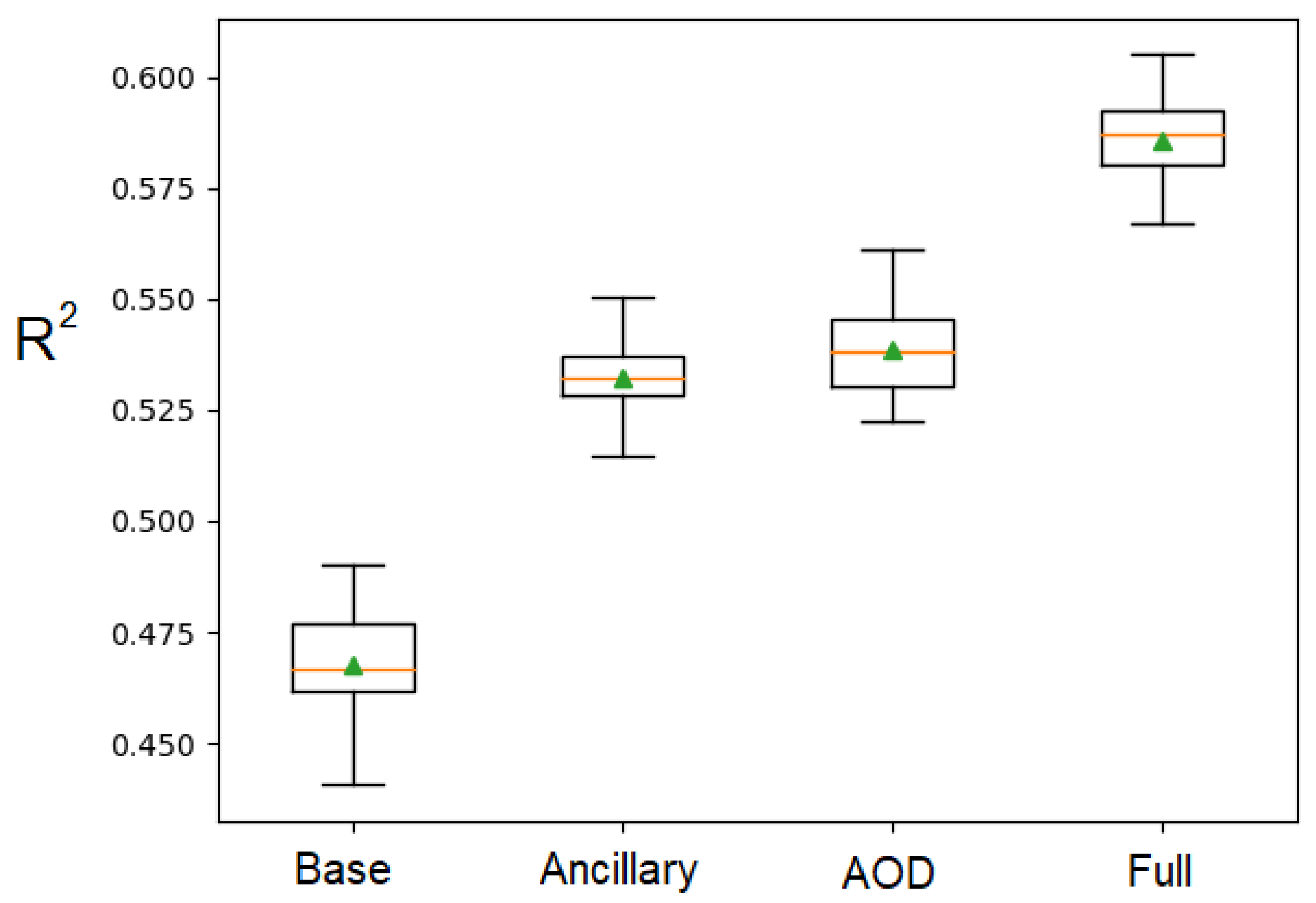
Four types of models with different predictor variables are established (Table 2). The hyper-parameters of these models are optimized through Bayesian Optimization based on 10-fold cross-validation. More specifically, the training dataset is divided into ten folds, nine of which are used to train the model and one fold is used for validation. In each hyper-parameter setting, the model performances are evaluated by repeating the 10-fold cross-validation process three times. The optimization process has 20 iterations, and 10 evaluations are made during each iteration. When the optimized hyper-parameters have been determined, the 10 R scores for each model type with the best hyper-parameter settings are plotted in Figure 5. The mean and standard deviation of the R scores are summarized in Table 2. The base model has the lowest R score of all four model types. Both ancillary data and the AOD product could improve the performance of the base model. The full model with all the variables has the highest overall R score. Once the best model type is identified, it will be trained on the entire training data with the optimized hyper-parameter settings.
Table 2.
Predictor variables sources as well as the 10-fold cross-validation results are listed. The Mean R represents the average value of the 10 R scores with the best hyper-parameter settings, and the STD represents the standard deviation of the 10 R scores for each model.
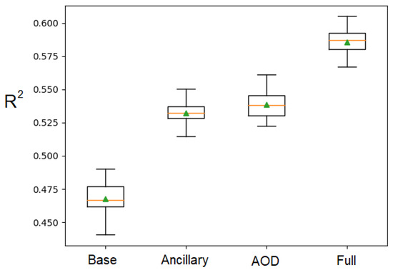
Figure 5.
Box plot for the R scores from the 10-fold cross-validation with the optimized hyper-parameters. The orange line represents the median; the green triangle represents the mean; the box represents the inter quantile range (IQR); top and bottom short lines correspond to the 1.5 IQR extension of the first and third quantiles, respectively.
A predictor importance rank chart is plotted once the model is finalized to illustrate the importance of all variables in the full model (see Figure 6; variable names can be found in Table 1). A tree model’s importance value indicates its ability to reduce impurities across the entire training dataset. Variables with a high importance score contribute more to model prediction than variables with a low importance score. As in the figure, the top 6 variables are AOD, temperature, dewpoint, boundary layer height, wind magnitude, and the month of the year.
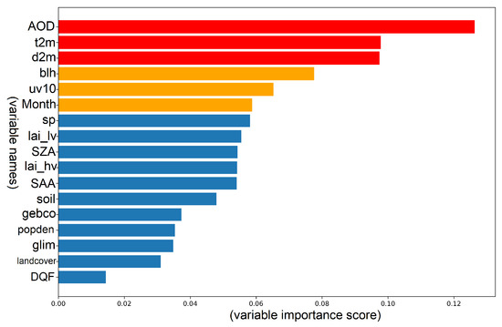
Figure 6.
The predictors importance plot. Red and orange bars represent the top six important variables. Names on the y-axis are the abbreviation for predictor variables and the values on the x-axis represent the importance score. These variables in this plot are described in Table 1.
3.2. Model Validation by Seasons
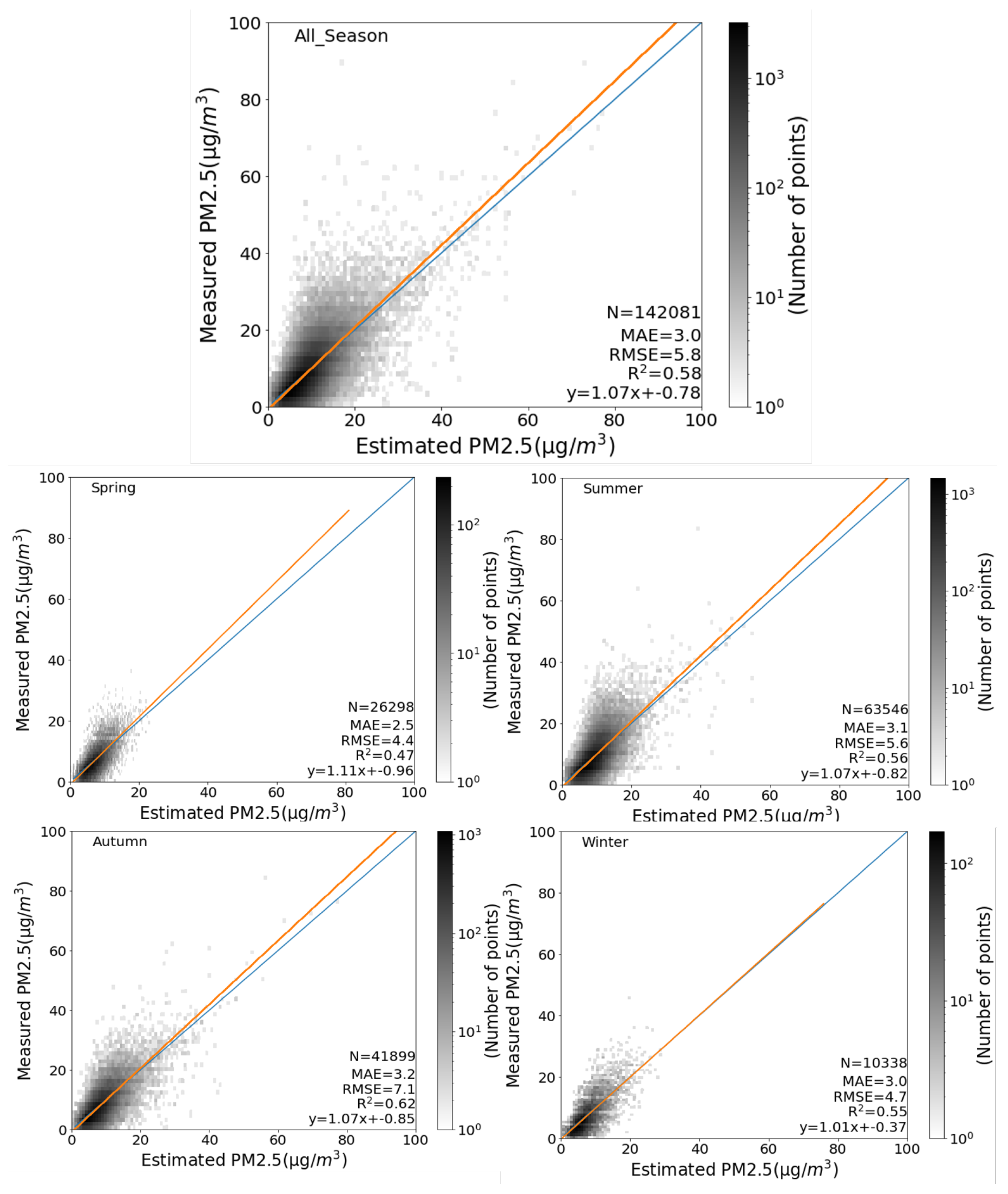
Once the model is finalized by training on the entire training dataset, it will be validated on the testing data in the temporal and spatial scale. Multiple scatter plots are generated between the estimated PM concentrations and the monitor measured PM values. There are a total of 142,081 PM values in the testing data set, and most of the values are within the range of 0 to 40. To better visualize the large number of overlapped points, the color-adjusted density distributions are represented by the power unit based on a color gradient from white to black.
Figure 7 displays the seasonal scatter diagrams. The overall performance of ET is reasonable, with MAE, RMSE, and R values of 3.0 g/m, 5.8 g/m, and 0.58, respectively. Based on these metrics, model performance varies from season to season. In Autumn, R reaches a maximum of 0.62 and decreases to 0.47 in Spring, whereas MAE and RMSE are relatively high in Autumn and low in Spring.
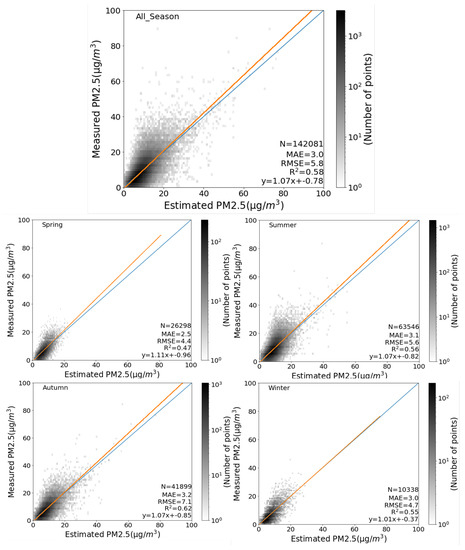
Figure 7.
The seasonal scatter diagrams on the testing dataset. The x-axis represents the estimated PM values and the y-axis represents the monitor measured PM values. Blue line and red line are the 1:1 reference line and the fit line, respectively. The gradient color from white to back represents different points densities. The four scatter diagrams are for the four seasons and the top one is for all seasons. N, MAE, RMSE, and R represent the number of observations, mean absolute error, root mean square error, and the determination of correlation coefficient, respectively.
To examine the spatial distribution of model estimation residuals, four MAE maps corresponding to the four seasonal scatter plots (Figure 7) are generated in Figure 8. The dots in the maps represent monitor stations, and the colors indicate their MAE values. The MAE distribution patterns varies with seasons. During the spring and winter, MAE values do not display high spatial variation, while high MAE clusters appear during the summer and autumn in California, Washington, and Montana. The most obvious MAE clusters in the three states are found in Autumn.
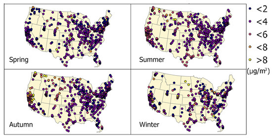
Figure 8.
The seasonal site based MAE maps. Different colors of dots represent the MAE values of each monitoring station. The four maps correspond to the station based MAE value distributions in Spring (March to May), Summer (June to August), Autumn (September to Nov), and Winter (December to February).
3.3. Model Validation by Time of Day
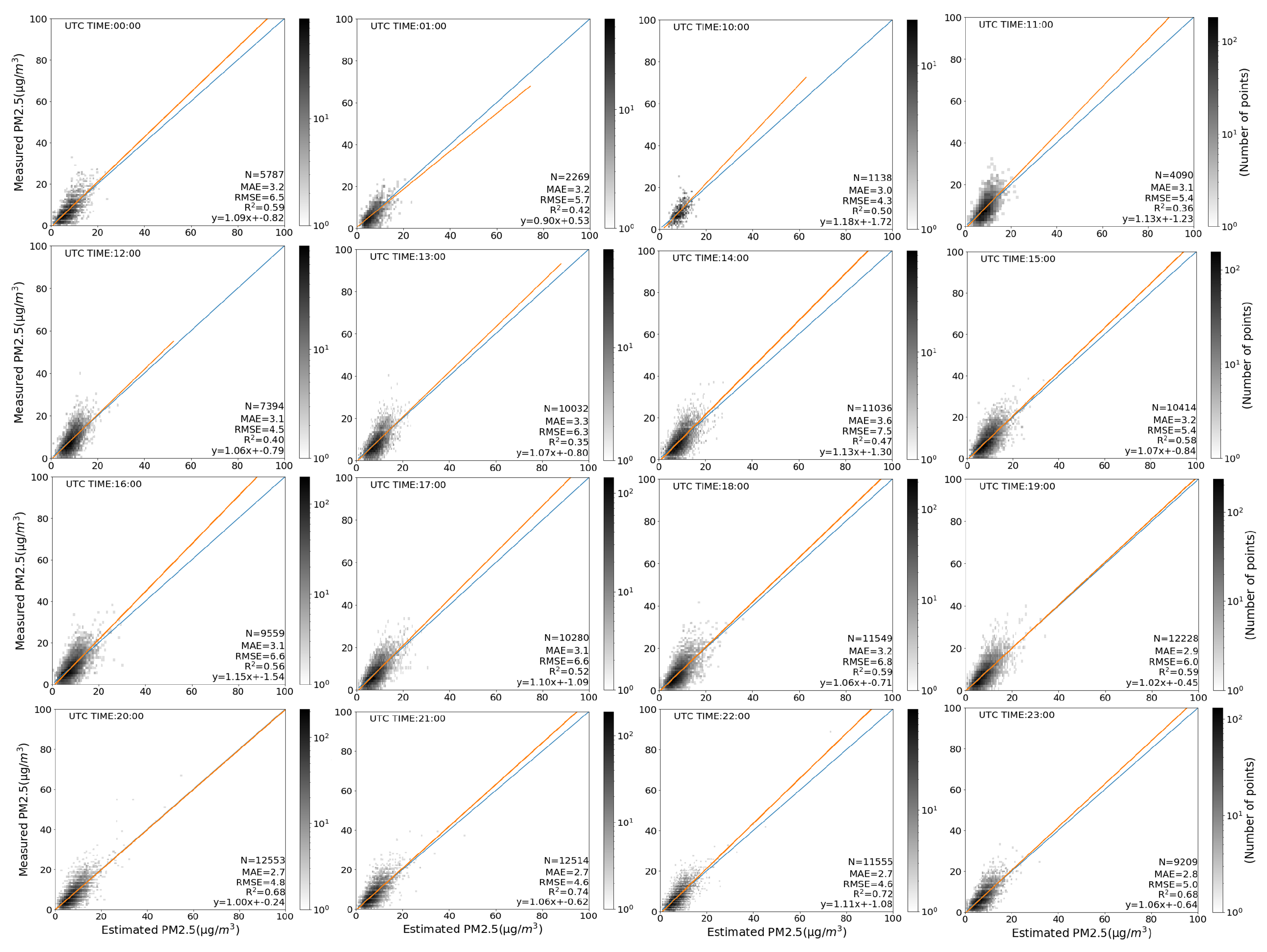
AOD from GOES-16 is only available during the daytime, and the quality and availability of data greatly depend on the time of day. Because of this, the model performance is analyzed according to the time of day in UTC. Sixteen of the 24 h are included for analysis, while the remaining eight hours (UTC: 2:00 a.m.–9:00 a.m.) are removed since AOD is not or barely available during these U.S. night hours. As in Figure 9, the values of R, MAE, RMSE range from 0.35 to 0.74, 2.7 to 3.6, and 4.3 to 7.5, respectively, at different hours. In terms of R scores, the model has the best performances at UTC 8:00 p.m.–11:00 p.m. (R) and has the worst performances at UTC 11:00 a.m.–1:00 p.m. (R). In terms of MAE, the model has the best performances at UTC 8:00 p.m.–11:00 p.m. (MAE ) and worst performances at UTC 1:00 p.m.–2:00 p.m. (MAE ). In terms of RMSE, the model has the best performance at UTC 10:00 a.m. with a RMSE of 4.3, and the worst performance at UTC 2:00 p.m. with a RMSE of 7.5.
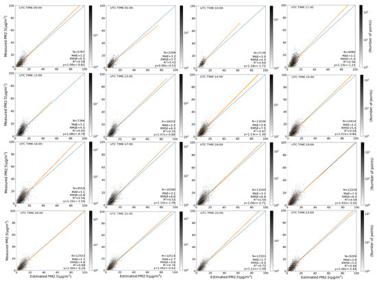
Figure 9.
Scatter diagrams (same as Figure 7) for the model estimations classified by the time of day. Each plot corresponds to an hour.
3.4. Model Validation by Ancillary Data
In this study, ancillary data are incorporated for PM estimation. Model performance metrics as well as monitoring stations distribution maps on elevation, population density, and landcover types are generated to better explore the relationship between ancillary data and model performance.
3.4.1. Model Validation by Elevation and Population Density
Population density and elevation have been investigated in relation to PM concentrations [44,45]. To better explore the model performance on these factors, the performance metrics as well as the ground observations are summarized in Table 3 and Table 4. Jenk’s natural break method was used to sort and divide the elevation and population density values of the 685 stations into six bins. The values in the Breaks column are the upper bounds of each bin and the unit is km for elevation bins and person/km for population density bins. Then, the measured mean (MM), MAE, RMSE, and R are calculated for each bin. N represents the number of observations from all the monitoring stations within each bin.
Table 3.
The model performance is summarized by elevation bins. Breaks are the upper bound of each bin and MM are the measured mean PM values. MAE, RMSE, and R are the model performance metrics for all sites in each bin. N represents the number of observations gathered from the sites in each bin.
Table 4.
The model performance summarized on population density bins. The meaning of MM, MAE, RMSE, R, and N are the same as in Table 3.
As in Table 3, the measured mean PM values are decreasing as the elevation value increases for the first four bins. For bins 5 and 6, the high elevation stations also have high mean measured PM values. For population density (Table 4), high population density bins are associated with high MM and R values for the first five bins. Bin 6 is an exception, as it has the highest population density, but the lowest MM and R values. An interesting observation is that high R scores are not always associated with low MAE and RMSE.
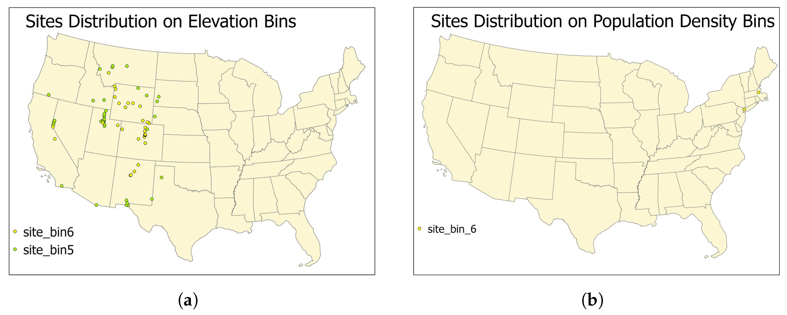
To better understand the bins with unusual high or low values, two maps are plotted in Figure 10 to show the spatial distributions of sites in these bins. Figure 10a shows the high-elevation stations with unusual high PM concentration values, which are located in the Rocky Mountains, New Mexico, and California. Stations with high population density are commonly near major cites and typically have higher PM concentrations than stations with low population density. However, the stations with high population density in bin6 are observed to have lower PM concentrations than expected. After investigating Figure 10b, it turns out that the two monitoring stations in bin 6 are located near New York City and Boston. Two factors can account for the population density and low MM values of bin 6 high. First, Bin 6 contains 230 samples, which is too few for representational validation. As a second reason, the two stations are located close to the east coast, where the coastal breeze alleviates the PM concentrations.
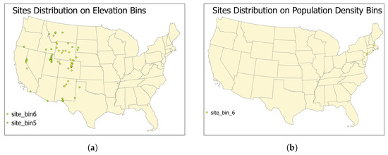
Figure 10.
The monitoring sites distributions. (a) shows the sites distributions for the two bins with the highest elevations; (b) shows the sites distributions for the bin with the highest population density.
3.4.2. Model Validation by Landcover
Landcover types have been identified as an important factor affecting PM concentrations [46]. For this reason, landcover data are collected from National Land Cover Database (NLCD) as a part of the PM study’s predictors. A total of 16 landcover types are included in the landcover dataset, which are regrouped into 8 main types in this study due to the similarity of some categories and the uneven distribution of samples in each category (see Table 5).
Table 5.
The model performance summarized on landcover types. The meaning of MM, MAE, RMSE, R, and N are the same as in Table 3.
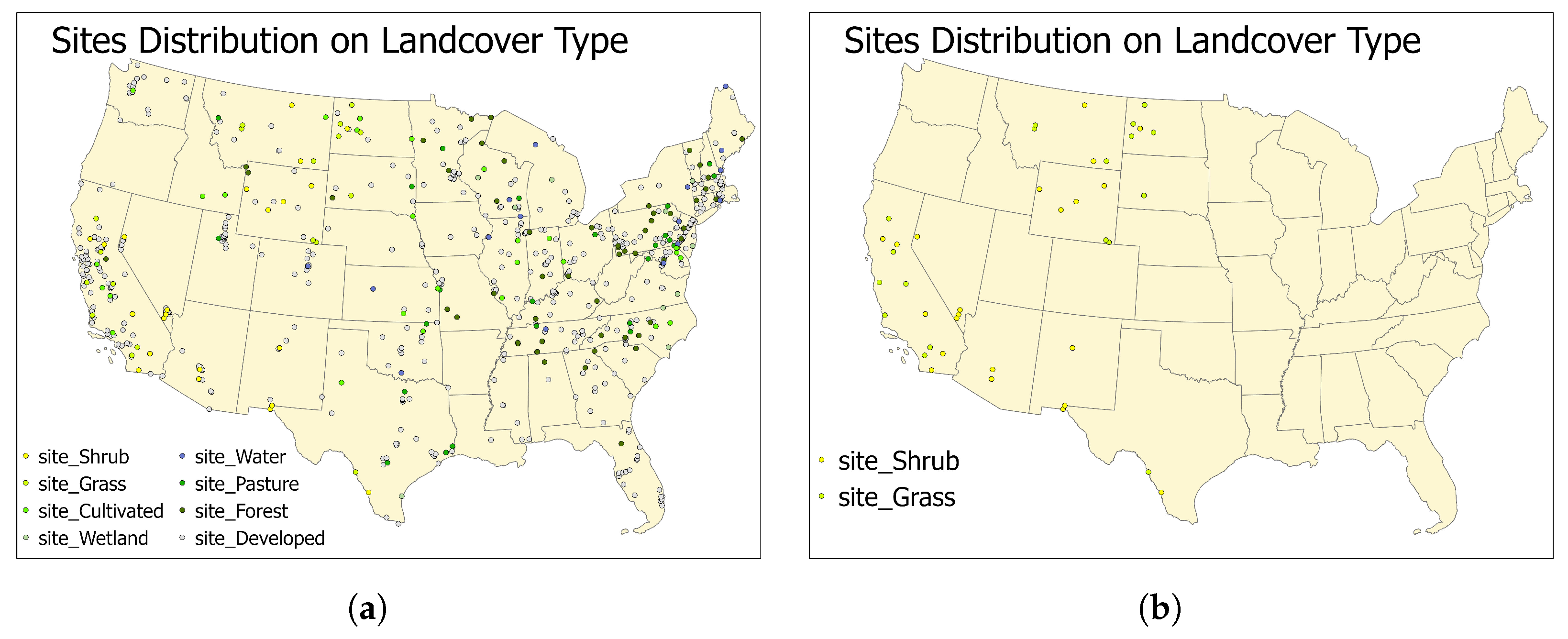
The machine learning model performance is evaluated by considering its landcover categories. According to Table 5, among the eight landcover types, water, forests, and wetlands have the lowest MM values, while cultivated crops, shrublands, and grasslands have the highest MM values. The developed category, which includes low, open space, medium intensity, and high intensity developed areas, ranks fourth in MM values. There is a direct correlation between high MM values and high MAE and RMSE across all land types. Although the value of MAE and RMSE are not found to be consistently related to R, the three largest R values (0.62, 0.6, 0.58) have been observed to be connected with the three large MM values (10.1 g/m, 8.8 g/m, 9.2 g/m). For a better understanding of how landcover types differ spatially, Figure 11 is plotted to show landcover type distributions. As in Figure 11a, forest, wetland stations are mainly in the east of the US; pasture and water stations are located in the middle and east of the country; cultivated and developed stations spread out the country; and shrubland and grassland are located in the west. Figure 11b shows the location of shrubland and grassland stations only. Shrubland and grassland have demonstrated the ability to sequester pollutants, thereby improving air quality [47]. However, the results found in this study contradict the theory due to the location of the shrubland and grassland stations. Training and testing data were collected from May 2017 to December 2020, a period during which 8 out of the top 20 fire events in California history occurred (see Table 6). Thus, those monitoring stations clustered in California that have specific landcover types have higher MM values than expected.
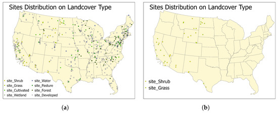
Figure 11.
The monitoring sites distributions by landcover types. (a) shows the sites distributions for all of the eight landcover types, and the (b) shows the sites distributions for the the two landcover types with the highest MM values.
Table 6.
The eight top ranked fire events in California between July 2017 and December 2020.
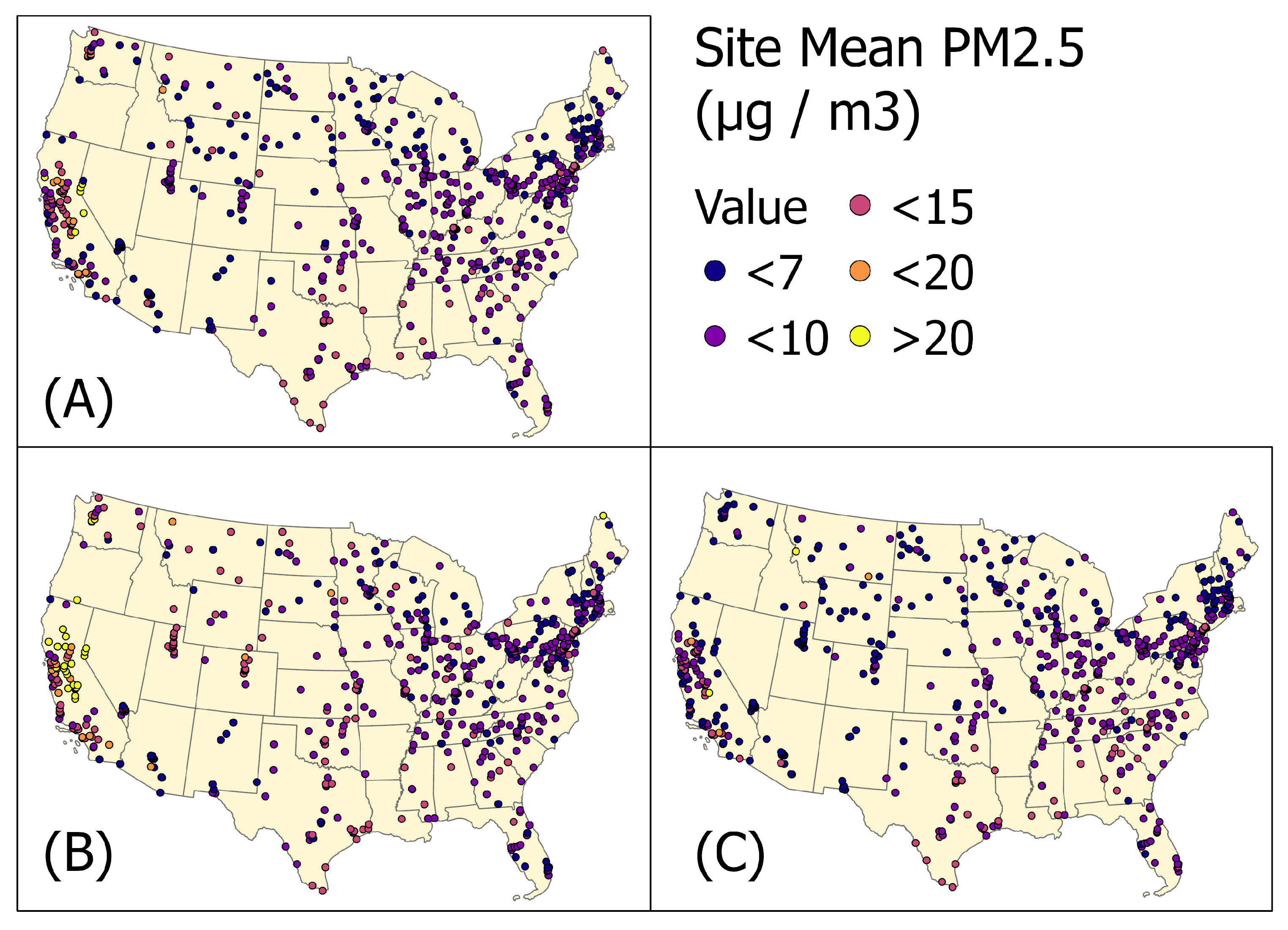
According to the results, sites within or near California tend to have higher MM values. Some of these can be attributed to population density and elevation, but some can be caused by fire events. PM data that are collected during California fire events between May 2017 and December 2020 have been separated from others to investigate the effect of fires on MM values. Figure 12A shows the measured mean PM concentrations for each site, including observations with and without fire events. In California, there are the highest site values, as well as the largest number of high value sites. Then, the observations during the period of fire events (Table 6) are separated and plotted in Figure 12B. Sites in California have a significant amount of high PM sites, as shown in the map. Figure 12C shows the mean site values during the period without fire events. As shown in the map, after excluding the observations during the California fire periods, mean site values have dropped significantly compared to those in Figure 12A.
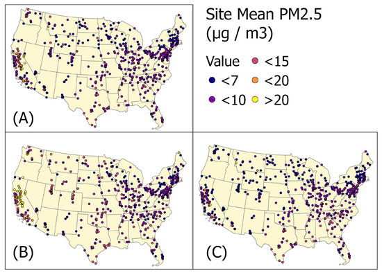
Figure 12.
The site measured mean PM values in fire and non-fire cases during July 2017 to December 2020. (A) is the measured mean values for all time; (B) is the measured mean values during fire events; and (C) is the measured mean values for the period without fire events.
The measured PM of each site with and without the California fires are summarized in Table 7, respectively. During fire periods, the site mean PM values are significantly higher than the value during non-fire periods. This agrees with the map in Figure 12.
Table 7.
The mean, median, and standard deviation (g/m) of the measured PM values, which are calculated during the period of fire only, non-fire, and all time. These metrics are summarized in CA and Nationwide, respectively.
3.5. PM Reconstruction and Fire Events Visualization
The study’s primary innovation is the use of the AOD product from the GOES-16 geostationary satellite, which allows the reconstruction of PM at a high temporal and spatial resolution during the daytime. Although the AOD products from polar orbit satellites, such as MODIS and VIIRS, also have high spatial resolution, their coarse temporal resolution makes them only ideal for modeling, but not for PM estimation in a high temporal manner. The temporal and spatial resolutions for the common instruments are summarized in Table 8.
Table 8.
AOD product platforms and instruments are summarized. Geos represents Geostationary orbit.
In this section, the established machine learning model is used to reconstruct the daytime hourly PM concentrations on 10 km by 10 km grids between 2017 and 2020. Due to large spatial coverage gaps in AOD data, the reconstructed PM surfaces prior to 2018 have been removed. Raw outputs cover the daytime period of the US at hourly intervals. However, the area covered varies significantly by time of day. Therefore, a daily and monthly average is derived from the hourly estimations. The air quality has been impacted by several fires that top the California fire history ranking in the years between 2017 and 2020 (see Table 6). Depending on the fire emissions and atmosphere condition, fire can inject a long distance into the air and migrate with wind. A large area could be polluted, and chronic diseases’ risks would increase [48,49,50]. Four of these fires occurred between July and October of 2020. Therefore, PM surfaces during this time range are constructed at hourly intervals to track the air pollution caused by fire, which serve as a valuable data source for studies related to fire pollution and human health. The hourly PM reconstruction surfaces are then averaged daily and monthly to capture the PM concentrations dynamically as the fire propagates.
Map visual interpretation can be affected by the color bar range selection. According to the WTO guide, the PM concentration above 25 g/m in 24 h mean could cause a high risk of health effect [51]. Thus, the 25 g/m is used as the upper bound for visualization, which also turns out to be effective to separate fire related high PM concentration zones from others.
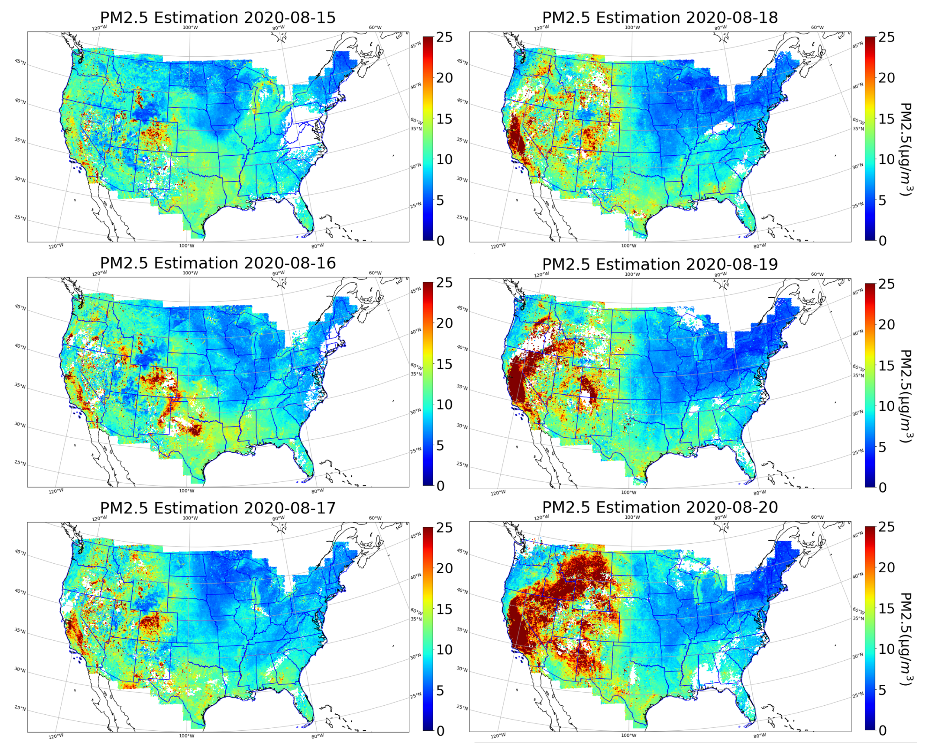
The Santa Clara Unit (SCU) Lightning Complex fire is the third largest fire in California history, which is ignited by dry lightning. It started on 16 August and was contained in early October. Figure 13 includes the reconstructed PM estimation surfaces on the several days before and after the start of the fire. As in the figure, the PM estimation surface on the 15th does not have obvious high pollution zones before the fire starts. The estimated surfaces on 16 January and 17 January, at the time of the lightning strikes, show some high PM concentration spots in California. Starting from the 18th, the high PM concentration zones are expanding and migrating to the states in the northeast direction on the 19th and 20th. On 19 August, a high concentration zone was captured in Colorado, which corresponds with the fact that Deter-Winters and Shamrock fires occurred on the same day in Colorado.
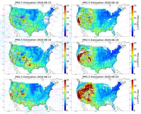
Figure 13.
The 10 km × 10 km daily averaged PM reconstruction surfaces from 15th to 20th of August 2020. Red colors depict the area with PM concentration above the 25 g/m threshold.
Figure 14 shows a set of monthly averaged PM estimation surfaces covering the SCU Lightning Complex. The SCU Lightning Complex fire started in August, and the estimated surface in August indicates a high concentration of PM in California, and extends to the western states. Deter-Winters and Shamrock, two smaller Colorado fire events, are also captured as small red patches. As the SCU Complex fire spreads in September, the polluted area reaches the maximum, including Washington, Montana, Wyoming, Arizona, Utah, Colorado, among others. In addition, in September, two additional fire events named Middle Fork and East Troublesome occurred in Colorado and resulted in high PM concentrations on the map. Having contained the SCU Lightning Complex fire in October, the fire’s impact (yellow on map) on the high PM area has been dramatically reduced. In November, the fire’s influence on air quality is almost gone and most states are back to their normal PM levels.
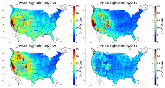
Figure 14.
The 10 km × 10 km monthly averaged PM reconstruction surfaces in August, September, October, and November in 2020.
4. Discussion
In this study, the hourly PM concentrations from in situ monitoring observations as well as meteorological variables from ECMWF analyses, remotely sensed GOES-16 AOD, and ancillary data from May 2017 to December 2020 are utilized for machine learning model training. The extra tree is employed due to its satisfactory performance in previous studies and its high computational efficiency. Comparing the four models with different predictor variables using the 10-fold cross validation, AOD and the variables from ancillary data were found to be able to improve the model performance significantly. Among all the variables, the AOD, temperature, dewpoint, wind magnitude, and boundary layer height have the most contributions to the model prediction, and the ancillary data as well as solar angles also contribute to the model performance. The finalized model has an overall performance of 3.0 g/m, 5.8 g/m, and 0.58 as of MAE, RMSE, and R on the testing dataset. During the validation process, the monitoring sites in the west-coast and north-west have higher MAE values than the other monitoring sites. The MAE and RMSE tend to be higher in winter than in other seasons. Analyzed by the time of day, the model performs best from 8:00 p.m. to 11:00 p.m. UTC (afternoon in north America). As a result of evaluating based on ancillary data, it appears that the measured mean PM concentration values of each monitoring site are positively related to the population density and negatively related to the elevation. Some of the exceptions with unusual high or low PM values can be explained by the fire events in high elevation area, as well as the special meteorological conditions in near sea locations. The lowest site mean PM values are associated with water, forest, and wetland landcover types, whereas developed, cultivated crop, shrub, and grass are associated with the highest PM concentrations. After investigating the spatial distribution of shrubland and grassland, the unusual high PM concentrations are related to a series of wildfires that happened in California between 2017 and 2020. Furthermore, the model MAE, RMSE, and R scores are positively correlated with the MM values of each site, which challenges the expectation that high R is always correlated with low MAE and RMSE. The results are consistent with many previous studies, which have shown that studies in high PM areas (such as China) tend to achieve higher model R scores than those in low PM areas (such as US).
The established machine learning model allows reconstruction of PM estimation surfaces at the hourly, daily, and monthly levels. These estimated surfaces are important data sources for PM monitoring, especially in tracking the PM changes in a high temporal manner. The reconstructed PM estimation surfaces during the California fire event match the timeline of the SCU Lightning Complex fire propagation process. There are several monitoring sites showing unusually high levels of PM, which appear to have been affected by the fire, including the high elevation sites in Figure 10a and the shrub/grass landcover sites in Figure 11b.
5. Conclusions
Many factors influence PM concentrations, including, but not limited to, meteorological conditions, democratic features, topography environments, and geological circumstances. The relationship between these factors and PM concentrations varies significantly in time and space. Therefore, the inclusion of ancillary data describing these factors over a period as long as possible is essential for developing a robust PM and representative model. GOES-16’s AOD product is another important data source that can enhance model performance. Its geostationary characteristics also allow the reconstruction of PM estimation surfaces in a highly dynamic manner, which is very beneficial for tracking air pollution events, such as wildfires. The comprehensive spatial coverage and the high temporal resolution of meteorological variables from ECMWF and AOD make the reconstruction of historical PM surfaces possible. These reconstructed PM surfaces become an important data source for those air pollution related epidemiological studies, such as asthma and acute respiratory distress. Compared to traditional PM monitoring sites, these reconstructed PM surfaces are continuous in space with a high frequency in time.
Author Contributions
Conceptualization, X.Y. and D.J.L.; methodology, X.Y. and D.J.L.; software, X.Y. and C.S.S.; validation, X.Y.; formal analysis, X.Y.; investigation, X.Y.; resources, X.Y., C.S.S. and D.J.L.; data curation, X.Y.; writing—original draft preparation, X.Y.; writing—review and editing, D.J.L.; visualization, X.Y. and C.S.S.; supervision, D.J.L.; project administration, X.Y. and D.J.L.; funding acquisition, D.J.L. and C.S.S. All authors have read and agreed to the published version of the manuscript.
Funding
This research was funded by National Science Foundation CNS Division Of Computer and Network Systems grant 1541227, and EPA Grant Number 83996501. The APC was funded by Christopher S. Simmons.
Institutional Review Board Statement
Not applicable.
Informed Consent Statement
Not applicable.
Data Availability Statement
The Python code for data preparation and modeling of this paper is available at URL: https://github.com/xiaoheyu (accessed on 22 November 2021). The links and APIs for data retrievals are available at URL: https://github.com/xiaoheyu/PM25-DataSource (accessed on 22 November 2021).
Acknowledgments
Christopher Simmons is gratefully acknowledged for his computational support. The authors acknowledge the Texas Research and Education Cyberinfrastructure Services (TRECIS) Center, NSF Award #2019135, and the University of Texas at Dallas for providing HPC, visualization, database, or grid resources and support that have contributed to the research results reported within this paper. URL: https://trecis.cyberinfrastructure.org/ (accessed on 28 October 2021). The authors acknowledge the Texas Advanced Computing Center (TACC) at the University of Texas at Austin for providing HPC, visualization, database, or grid resources that have contributed to the research results reported within this paper. URL: http://www.tacc.utexas.edu (accessed on 28 October 2021). This research received support from USAMRMC Award Number W81XWH-18-1-0400. National Science Foundation CNS Division Of Computer and Network Systems grant 1541227, and EPA Grant Number 83996501.
Conflicts of Interest
The authors declare no conflict of interest.
References
- Boucher, O. Atmospheric aerosols. In Atmospheric Aerosols; Springer: Berlin, Germany, 2015; pp. 9–24. [Google Scholar]
- Dubovik, O.; Holben, B.; Eck, T.F.; Smirnov, A.; Kaufman, Y.J.; King, M.D.; Tanré, D.; Slutsker, I. Variability of absorption and optical properties of key aerosol types observed in worldwide locations. J. Atmos. Sci. 2002, 59, 590–608. [Google Scholar] [CrossRef]
- Ramanathan, V.; Crutzen, P.; Kiehl, J.; Rosenfeld, D. Aerosols, climate, and the hydrological cycle. Science 2001, 294, 2119–2124. [Google Scholar] [CrossRef] [Green Version]
- Sun, Y.; Zhuang, G.; Tang, A.; Wang, Y.; An, Z. Chemical characteristics of PM2.5 and PM10 in haze-fog episodes in Beijing. Environ. Sci. Technol. 2006, 40, 3148–3155. [Google Scholar] [CrossRef] [PubMed]
- Zhang, R.; Tian, P.; Ji, Y.; Lin, Y.; Peng, J.; Pan, B.; Wang, Y.; Wang, G.; Li, G.; Wang, W.; et al. Overview of Persistent Haze Events in China. In Air Pollution in Eastern Asia: An Integrated Perspective; Springer: Berlin, Germany, 2017; pp. 3–25. [Google Scholar]
- Pope, C.A., III; Burnett, R.T.; Thun, M.J.; Calle, E.E.; Krewski, D.; Ito, K.; Thurston, G.D. Lung cancer, cardiopulmonary mortality, and long-term exposure to fine particulate air pollution. JAMA 2002, 287, 1132–1141. [Google Scholar] [CrossRef] [Green Version]
- Pope, C.A., III; Dockery, D.W. Health effects of fine particulate air pollution: Lines that connect. J. Air Waste Manag. Assoc. 2006, 56, 709–742. [Google Scholar] [CrossRef]
- Hua, J.; Yin, Y.; Peng, L.; Du, L.; Geng, F.; Zhu, L. Acute effects of black carbon and PM2.5 on children asthma admissions: A time-series study in a Chinese city. Sci. Total Environ. 2014, 481, 433–438. [Google Scholar] [CrossRef]
- Lim, S.S.; Vos, T.; Flaxman, A.D.; Danaei, G.; Shibuya, K.; Adair-Rohani, H.; AlMazroa, M.A.; Amann, M.; Anderson, H.R.; Andrews, K.G.; et al. A comparative risk assessment of burden of disease and injury attributable to 67 risk factors and risk factor clusters in 21 regions, 1990–2010: A systematic analysis for the Global Burden of Disease Study 2010. Lancet 2012, 380, 2224–2260. [Google Scholar] [CrossRef] [Green Version]
- Yu, W.; Liu, S.; Jiang, J.; Chen, G.; Luo, H.; Fu, Y.; Xie, L.; Li, B.; Li, N.; Chen, S.; et al. Burden of ischemic heart disease and stroke attributable to exposure to atmospheric PM2.5 in Hubei province, China. Atmos. Environ. 2020, 221, 117079. [Google Scholar] [CrossRef]
- Bartell, S.M.; Longhurst, J.; Tjoa, T.; Sioutas, C.; Delfino, R.J. Particulate air pollution, ambulatory heart rate variability, and cardiac arrhythmia in retirement community residents with coronary artery disease. Environ. Health Perspect. 2013, 121, 1135–1141. [Google Scholar] [CrossRef]
- Lary, M.A.; Allsopp, L.; Lary, D.J.; Sterling, D.A. Using machine learning to examine the relationship between asthma and absenteeism. Environ. Monit. Assess. 2019, 191, 332. [Google Scholar] [CrossRef]
- Clark, N.M.; Brown, R.; Joseph, C.L.; Anderson, E.W.; Liu, M.; Valerio, M.A. Effects of a comprehensive school-based asthma program on symptoms, parent management, grades, and absenteeism. Chest 2004, 125, 1674–1679. [Google Scholar] [CrossRef] [PubMed]
- Tsakiris, A.; Iordanidou, M.; Paraskakis, E.; Tsalkidis, A.; Rigas, A.; Zimeras, S.; Katsardis, C.; Chatzimichael, A. The presence of asthma, the use of inhaled steroids, and parental education level affect school performance in children. BioMed Res. Int. 2013, 2013, 762805. [Google Scholar] [CrossRef] [Green Version]
- EPA. Air Quality System (AQS) API. 2020. Available online: https://aqs.epa.gov/aqsweb/documents/data_api.html (accessed on 22 November 2021).
- Lary, D.J.; Alavi, A.H.; Gandomi, A.H.; Walker, A.L. Machine learning in geosciences and remote sensing. Geosci. Front. 2016, 7, 3–10. [Google Scholar] [CrossRef] [Green Version]
- Lary, D.J.; Zewdie, G.K.; Liu, X.; Wu, D.; Levetin, E.; Allee, R.J.; Malakar, N.; Walker, A.; Mussa, H.; Mannino, A.; et al. Machine Learning Applications for Earth Observation. In Earth Observation Open Science and Innovation; ISSI Scientific Report Series; Springer: Berlin, Germany, 2018; Volume 15, pp. 165–218. [Google Scholar]
- Zewdie, G.K.; Lary, D.J.; Liu, X.; Wu, D.; Levetin, E. Estimating the daily pollen concentration in the atmosphere using machine learning and NEXRAD weather radar data. Environ. Monit. Assess. 2019, 191, 418. [Google Scholar] [CrossRef] [PubMed]
- Wijeratne, L.O.; Kiv, D.R.; Aker, A.R.; Talebi, S.; Lary, D.J. Using Machine Learning for the Calibration of Airborne Particulate Sensors. Sensors 2020, 20, 99. [Google Scholar] [CrossRef] [PubMed] [Green Version]
- Lary, D.J.; Faruque, F.S.; Malakar, N.; Moore, A.; Roscoe, B.; Adams, Z.L.; Eggelston, Y. Estimating the global abundance of ground level presence of particulate matter (PM2.5). Geospat. Health 2014, 8, 611–630. [Google Scholar] [CrossRef]
- Lary, D.; Lary, T.; Sattler, B. Using Machine Learning to Estimate Global PM2.5 for Environmental Health Studies. Environ. Health Insights 2015, 1, 41–52. [Google Scholar] [CrossRef]
- Zang, Z.; Li, D.; Guo, Y.; Shi, W.; Yan, X. Superior PM2.5 Estimation by Integrating Aerosol Fine Mode Data from the Himawari-8 Satellite in Deep and Classical Machine Learning Models. Remote Sens. 2021, 13, 2779. [Google Scholar] [CrossRef]
- Liu, J.; Weng, F.; Li, Z.; Cribb, M.C. Hourly PM2.5 estimates from a geostationary satellite based on an ensemble learning algorithm and their spatiotemporal patterns over central east China. Remote Sens. 2019, 11, 2120. [Google Scholar] [CrossRef] [Green Version]
- Engel-Cox, J.A.; Hoff, R.M.; Haymet, A. Recommendations on the use of satellite remote-sensing data for urban air quality. J. Air Waste Manag. Assoc. 2004, 54, 1360–1371. [Google Scholar] [CrossRef]
- Hoff, R.M.; Christopher, S.A. Remote sensing of particulate pollution from space: Have we reached the promised land? J. Air Waste Manag. Assoc. 2009, 59, 645–675. [Google Scholar] [CrossRef] [PubMed]
- Song, W.; Jia, H.; Huang, J.; Zhang, Y. A satellite-based geographically weighted regression model for regional PM2.5 estimation over the Pearl River Delta region in China. Remote Sens. Environ. 2014, 154, 1–7. [Google Scholar] [CrossRef]
- Zheng, C.; Zhao, C.; Zhu, Y.; Wang, Y.; Shi, X.; Wu, X.; Chen, T.; Wu, F.; Qiu, Y. Analysis of influential factors for the relationship between PM2.5 and AOD in Beijing. Atmos. Chem. Phys. 2017, 17, 13473–13489. [Google Scholar] [CrossRef] [Green Version]
- Zhang, H.; Hoff, R.M.; Engel-Cox, J.A. The relation between Moderate Resolution Imaging Spectroradiometer (MODIS) aerosol optical depth and PM2.5 over the United States: A geographical comparison by US Environmental Protection Agency regions. J. Air Waste Manag. Assoc. 2009, 59, 1358–1369. [Google Scholar] [CrossRef] [Green Version]
- Yang, Q.; Yuan, Q.; Yue, L.; Li, T.; Shen, H.; Zhang, L. The relationships between PM2.5 and aerosol optical depth (AOD) in mainland China: About and behind the spatio-temporal variations. Environ. Pollut. 2019, 248, 526–535. [Google Scholar] [CrossRef]
- Drury, E.; Jacob, D.J.; Spurr, R.J.; Wang, J.; Shinozuka, Y.; Anderson, B.E.; Clarke, A.D.; Dibb, J.; McNaughton, C.; Weber, R. Synthesis of satellite (MODIS), aircraft (ICARTT), and surface (IMPROVE, EPA-AQS, AERONET) aerosol observations over eastern North America to improve MODIS aerosol retrievals and constrain surface aerosol concentrations and sources. J. Geophys. Res. Atmos. 2010, 115, D14204. [Google Scholar] [CrossRef] [Green Version]
- Just, A.C.; De Carli, M.M.; Shtein, A.; Dorman, M.; Lyapustin, A.; Kloog, I. Correcting measurement error in satellite aerosol optical depth with machine learning for modeling PM2.5 in the Northeastern USA. Remote Sens. 2018, 10, 803. [Google Scholar] [CrossRef] [Green Version]
- Li, L. A robust deep learning approach for spatiotemporal estimation of satellite AOD and PM2.5. Remote Sens. 2020, 12, 264. [Google Scholar] [CrossRef] [Green Version]
- Li, T.; Shen, H.; Yuan, Q.; Zhang, X.; Zhang, L. Estimating ground-level PM2.5 by fusing satellite and station observations: A geo-intelligent deep learning approach. Geophys. Res. Lett. 2017, 44, 11–985. [Google Scholar] [CrossRef] [Green Version]
- Jung, C.R.; Chen, W.T.; Nakayama, S.F. A National-Scale 1-km Resolution PM2.5 Estimation Model over Japan Using MAIAC AOD and a Two-Stage Random Forest Model. Remote Sens. 2021, 13, 3657. [Google Scholar] [CrossRef]
- Schneider, R.; Vicedo-Cabrera, A.M.; Sera, F.; Masselot, P.; Stafoggia, M.; de Hoogh, K.; Kloog, I.; Reis, S.; Vieno, M.; Gasparrini, A. A satellite-based spatio-temporal machine learning model to reconstruct daily PM2.5 concentrations across Great Britain. Remote Sens. 2020, 12, 3803. [Google Scholar] [CrossRef]
- Tang, Y.; Deng, R.; Li, J.; Liang, Y.; Xiong, L.; Liu, Y.; Zhang, R.; Hua, Z. Estimation of Ultrahigh Resolution PM2.5 Mass Concentrations Based on Mie Scattering Theory by Using Landsat8 OLI Images over Pearl River Delta. Remote Sens. 2021, 13, 2463. [Google Scholar] [CrossRef]
- Geng, G.; Zhang, Q.; Martin, R.V.; van Donkelaar, A.; Huo, H.; Che, H.; Lin, J.; He, K. Estimating long-term PM2.5 concentrations in China using satellite-based aerosol optical depth and a chemical transport model. Remote Sens. Environ. 2015, 166, 262–270. [Google Scholar] [CrossRef]
- Beckerman, B.S.; Jerrett, M.; Serre, M.; Martin, R.V.; Lee, S.J.; Van Donkelaar, A.; Ross, Z.; Su, J.; Burnett, R.T. A hybrid approach to estimating national scale spatiotemporal variability of PM2.5 in the contiguous United States. Environ. Sci. Technol. 2013, 47, 7233–7241. [Google Scholar] [CrossRef] [PubMed] [Green Version]
- Wu, D.; Lary, D.J.; Zewdie, G.K.; Liu, X. Using machine learning to understand the temporal morphology of the PM2.5 annual cycle in East Asia. Environ. Monit. Assess. 2019, 191, 272. [Google Scholar] [CrossRef] [PubMed]
- Liu, X.; Wu, D.; Zewdie, G.K.; Wijerante, L.; Timms, C.I.; Riley, A.; Levetin, E.; Lary, D.J. Using machine learning to estimate atmospheric Ambrosia pollen concentrations in Tulsa, OK. Environ. Health Insights 2017, 11, 1178630217699399. [Google Scholar] [CrossRef] [Green Version]
- Breiman, L. Random forests. Mach. Learn. 2001, 45, 5–32. [Google Scholar] [CrossRef] [Green Version]
- Bin, C.; Song, Z.; Pan, F.; Huang, Y. Obtaining vertical distribution of PM2.5 from CALIOP data and machine learning algorithms. Sci. Total Environ. 2021, 805, 150338. [Google Scholar]
- Geurts, P.; Ernst, D.; Wehenkel, L. Extremely randomized trees. Mach. Learn. 2006, 63, 3–42. [Google Scholar] [CrossRef] [Green Version]
- Han, S.; Sun, B. Impact of population density on PM2.5 concentrations: A case study in Shanghai, China. Sustainability 2019, 11, 1968. [Google Scholar] [CrossRef] [Green Version]
- Alvarez, H.B.; Echeverria, R.S.; Alvarez, P.S.; Krupa, S. Air quality standards for particulate matter (PM) at high altitude cities. Environ. Pollut. 2013, 173, 255–256. [Google Scholar] [CrossRef] [PubMed]
- Yang, W.; Jiang, X. Evaluating the influence of land use and land cover change on fine particulate matter. Sci. Rep. 2021, 11, 17612. [Google Scholar] [CrossRef] [PubMed]
- Gopalakrishnan, V.; Hirabayashi, S.; Ziv, G.; Bakshi, B.R. Air quality and human health impacts of grasslands and shrublands in the United States. Atmos. Environ. 2018, 182, 193–199. [Google Scholar] [CrossRef] [Green Version]
- Langmann, B.; Duncan, B.; Textor, C.; Trentmann, J.; Van Der Werf, G.R. Vegetation fire emissions and their impact on air pollution and climate. Atmos. Environ. 2009, 43, 107–116. [Google Scholar] [CrossRef]
- Hayasaka, H.; Noguchi, I.; Putra, E.I.; Yulianti, N.; Vadrevu, K. Peat-fire-related air pollution in Central Kalimantan, Indonesia. Environ. Pollut. 2014, 195, 257–266. [Google Scholar] [CrossRef]
- Marlier, M.E.; DeFries, R.S.; Voulgarakis, A.; Kinney, P.L.; Randerson, J.T.; Shindell, D.T.; Chen, Y.; Faluvegi, G. El Niño and health risks from landscape fire emissions in southeast Asia. Nat. Clim. Chang. 2013, 3, 131–136. [Google Scholar] [CrossRef] [Green Version]
- World Health Organization. Air Quality Guidelines: Global Update 2005: Particulate Matter, Ozone, Nitrogen Dioxide, and Sulfur Dioxide; World Health Organization: Geneva, Switzerland, 2006. [Google Scholar]


Publisher’s Note: MDPI stays neutral with regard to jurisdictional claims in published maps and institutional affiliations. |
© 2021 by the authors. Licensee MDPI, Basel, Switzerland. This article is an open access article distributed under the terms and conditions of the Creative Commons Attribution (CC BY) license (https://creativecommons.org/licenses/by/4.0/).