Using Electrical Resistivity Tomography to Monitor the Evolution of Landslides’ Safety Factors under Rainfall: A Feasibility Study Based on Numerical Simulation

Abstract

Although electrical resistivity tomography (ERT) may gather the internal resistivity information from a landslide area in a large-scale, low-cost, and non-invasive manner compared to point-based sensor monitoring technology, the indirect resistivity information obtained cannot directly evaluate the landslide’s current mechanical status, such as stress, strength, etc. Based on ERT monitoring data, a framework for quantitatively and directly evaluating the evolution of the factor of safety (FOS) of landslides during rainfall is proposed. The framework first inverts ERT observation data using the inexact Gauss–Newton method based on multiple constraints to obtain a more realistic resistivity distribution, then calculates the saturation distribution using Archie’s equation, and finally calculates the FOS of landslides using the finite element strength reduction method. Twelve sets of numerical experiments were designed and carried out based on the synthetic data of a theoretical model. The experimental results show that the proposed framework is valid and reliable under various arrays, apparent resistivity noise, and uncertainty in the water-electric correlation curve, with the Dipole-Dipole array outperforming the others in terms of accuracy, sensitivity, and anti-noise capability. The proposed framework is significant in improving ERT monitoring and early warning capabilities for rainfall-induced landslides.

1. Introduction

With the hilly landforms and abundant rainfall in southern China [1,2], a large number of landslides occur every year during the rainy season, resulting in numerous fatalities and significant economic losses [3]. Rainfall infiltration not only causes the weight of the soil to grow and the driving shear force to increase, but also causes the landslide soil mechanics to change and the resistant shear force to diminish due to interaction with water within the landslide body displacement; failure can even occur once the driving shear force exceeds the resistant shear force [4]. Monitoring the spatial and temporal evolution of water content inside landslides under rainfall conditions and analyzing their effects on geotechnical behavior are important for early warning of landslides. The water inside landslides is currently monitored primarily using point-based sensors such as water level meters and seepage pressure meters [5,6,7], which can continuously and accurately obtain hydrological parameters such as pore water pressure and substrate matrix suction at the sensor location, but there are two drawbacks: First, geotechnical parameters, particularly hydrological parameters, are spatially variable [8,9,10], and point-based sensors often only reflect information about the sensor’s immediate surroundings, with limited ability to sense information further away. Second, such sensors frequently require drilling holes in the landslide body, which can be difficult and costly to implement. In some cases, the “destructive” activities can even cause movements or failures of landslides.

Numerous studies have shown that the electrical conductivity of the soil is closely related to the water content of the soil [11,12,13,14,15]. Rainfall can change the water content of landslides in both space and time, and because water content and resistivity are correlated, it will also change the resistivity of landslides. Based on this idea, electrical resistivity tomography (ERT) with resistivity as the primary parameter was used to characterize and study the spatiotemporal distribution of water content inside a landslide [16,17,18]. The ERT images the distribution of resistivity parameters in the subsurface by injecting current on the surface or in the boreholes and then collecting the potential distribution. The correlation between resistivity and water content allows the technique to be used to indirectly reflect the distribution of subsurface water content [19,20]. In comparison to point-based sensor monitoring, ERT can acquire internal resistivity information about landslides in a greater region in a non-invasive manner. The benefits of ERT are the simplicity of field operation and the low cost of data acquisition.

An increasing number of research works in recent years have achieved many very valuable and representative results in characterizing and monitoring information such as internal resistivity and water content associated with resistivity of landslides based on ERT [21,22,23]. Geng et al. [24], Liu et al. [25], Hojat et al. [26], and Lyu et al. [27] established physical models and completed experiments in the laboratory to monitor the geoelectric field response during rainfall infiltration. The results of these experiments verified the correlation of electrical parameters such as self-potential and primary field potential with the spatial and temporal distribution of moisture. Zeng et al. [28], Uhlemann et al. [29], Boyle et al. [30], Whiteley et al. [19], Denchik et al. [31], and Boyd et al. [32] installed ERT devices on actual landslides and combined drilling, mapping, and other data to investigate the internal water transport of landslides under rainfall conditions and its impact on landslide failure. Manoli et al. [33], Carey et al. [34], and Hojat et al. [26] used numerical simulation approaches to compute and assess the geoelectric field response characteristics of the soil during rainfall infiltration. Through indoor experiments, actual case studies, and numerical simulations, these works demonstrate how ERT approaches can be utilized to quantify and monitor water transport within landslides, and hence qualitatively investigate landslide failure processes. However, because ERT data indirectly reflect information such as water content and stress state within a landslide and cannot intuitively correlate with landslide geotechnical behavior, it is worthwhile to investigate how to use ERT data for landslide activity evaluation and early warning. Crawford et al. [35,36,37] offered a comprehensive framework for establishing a relationship between ERT data and landslide shear strength, providing a highly significant investigation of the use of ERT data for landslide early warning. The factor of safety (FOS) of a landslide is a more straightforward parameter to evaluate the stability of a landslide than shear strength. It can provide a more straightforward early warning effect if ERT monitoring data can be used to dynamically depict the change in FOS of landslides under rainfall conditions.

In this paper, a framework for using ERT observation data to reflect the change in FOS of landslides during rainfall was proposed. In the proposed framework, synthetic data are first obtained by forward modeling of a specific landslide model. Then, the inexact Gauss–Newton inversion algorithm based on multiple constraints is applied to the synthetic data to analyze the spatial and temporal distribution of the resistivity. After that, the distribution of moisture can be obtained with the help of the relationship between resistivity and water content constructed by the water–electricity correlation curve (WECC). Finally, the FOS of the landslide can be calculated by using the strength reduction method (SRM) using COMSOL software. Twelve sets of numerical simulation experiments for a theoretical model with the proposed framework were completed, and the effects of the proposed framework on computed FOS under various arrays, apparent resistivity noise, and WECC uncertainty were investigated to verify the proposed framework’s performance and reliability.

2. Methodology

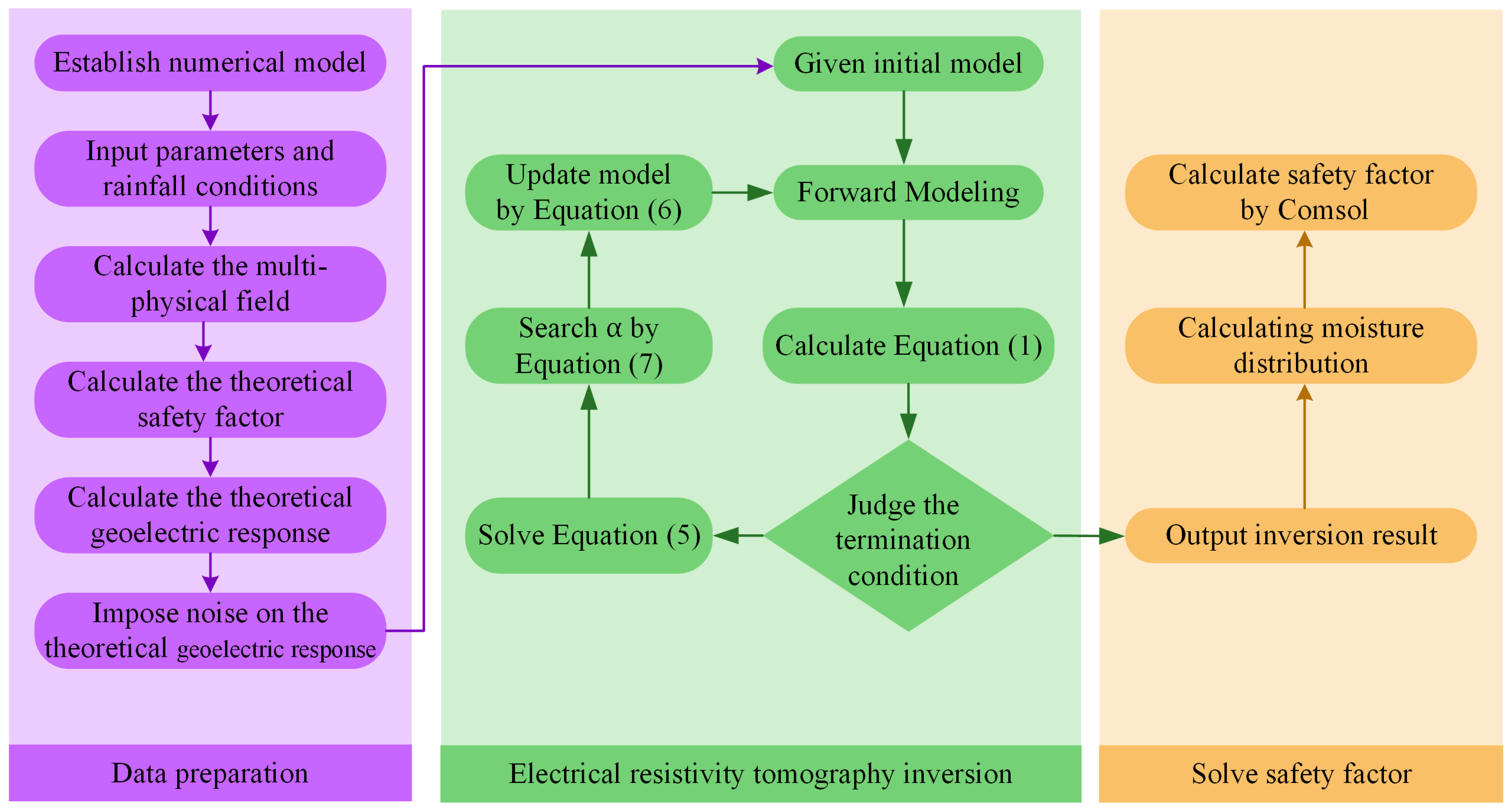
The proposed framework for calculating the FOS of landslides during rainfall using ERT observation data is shown in Figure 1. In the data preparation section, the synthetic data from the forward modeling of the theoretical model was chosen as the data source due to the lack of real measurement data and the need for a controlled and quantitative evaluation of the reliability of different scenarios. Firstly, a numerical model should be established and given the basic parameters and rainfall conditions, COMSOL software is used to calculate the spatial and temporal response of the seepage field, stress field, and the evolution of the theoretical FOS for this model under the specified rainfall conditions. The seepage fields are then transformed into resistivity distributions using various WECCs, and the apparent resistivity responses of various arrays are calculated and saved to be used as input data for the proposed framework. The proposed framework first calculates the resistivity distribution for synthetic data using the inexact Gauss–Newton inversion based on multiple constraints, then calculates the moisture distribution using the fitted WECC, and finally calculates the predicted FOS in COMSOL using SRM, which is compared and analyzed with the theoretical FOS calculated in the data preparation section to verify the feasibility, sensitivity, and anti-noise capability. The inversion is the most significant aspect of this framework. Multiple constraints, such as the prior model constraint, model smoothness constraint, and regularization constraint, are needed for the inversion process to increase the accuracy of the inversion due to the unique properties of landslides under rainfall conditions. The inversion process utilizes the inexact Gauss–Newton method [38] to determine the search direction, the Wolfe criterion [38] to determine the iteration step, and the Jacobian-free Krylov solution technique [39] to avoid the direct calculation of large, dense Jacobian matrices, all of which improve inversion efficiency.

2.1. Inexact Gauss–Newton Inversion Algorithm Based on Multiple Constraints

Geophysical inversion is a technique that uses observed data to infer the spatial distribution of subsurface physical parameters [40,41]. However, because the observed data are limited, the inverse problem is usually ill-posed, and the inversion results frequently have issues such as instability and non-uniqueness [40,41]. To minimize the ill-posed problem, Tikhonov et al. [42] proposed a regularized inversion method to stabilize the model iteration process by adding a regularized model constraint term to the inversion objective function. The regularization objective function used in this paper is:

$$\mathsf{\phi }={\mathsf{\phi }}_d+\lambda {\mathsf{\phi }}_m=\frac{1}{2}{\Vert D(A(m)-d_{obs})\Vert }^2+\frac{\lambda }{2}{\Vert W(m-m_{apr})\Vert }^2$$

(1)

where $\mathsf{\phi }$ denotes the inversion’s objective function, which is made up of two parts: the data item ${\mathsf{\phi }}_d=\frac{1}{2}{\Vert D(A(m)-d_{obs})\Vert }^2$ and the regularized model item $\lambda {\mathsf{\phi }}_m=\frac{\lambda }{2}{\Vert W(m-m_{apr})\Vert }^2$. $\lambda$ denotes the regularization parameter, $D$ denotes the observed data weight, $W$ denotes the model weight, $A$ denotes the forward modeling operator, $m_{apr}$ denotes the reference model given based on a priori information, $d_{obs}$ denotes the observed data, and $m$ denotes the model vector to be solved. where the regularization parameter $\lambda$ is set to 0.05 in the early stage and the following equation is used for adaptive dynamic computation in the later stage:

$${\lambda }^{(k)}=\frac{{\mathsf{\phi }}_d^{(k-1)}}{{\mathsf{\phi }}_d^{(k-1)}+{\mathsf{\phi }}_m^{(k-1)}}\mathbf{·}\frac{{\mathsf{\phi }}_d^{(k-1)}}{{\mathsf{\phi }}_d^{(k-2)}}$$

(2)

where k denotes the current number of iterations. When compared to approaches such as L-Curve [43], this calculation method may utilize the results of previous iterations and does not require a duplicated forward modeling step, which considerably reduces the computational burden and time consumption.

The data weight matrix $D$ is calculated using the following equation [38]:

$$D=\mathrm{diag}\left(\frac{1}{\left|d_{\mathrm{obs}}\right|\cdot SD\left(d_{\mathrm{obs}}\right)+\epsilon }\right)$$

(3)

where $SD\left(d_{\mathrm{obs}}\right)$ denotes the observed data’s standard deviation and $\epsilon$ denotes the smallest possible data value to keep the denominator term from converging to zero, usually 0.0125.

Model weights $W$ can place smooth constraints on the inversion process and ensure the inversion model’s spatial continuity [39].

$$W=\{\begin{array}{c}\begin{array}{cc}-\frac{1}{r_{ij}}/{\displaystyle \sum _{j=1}^{k_i}\frac{1}{r_{ij}}}& i \mathrm{and} j \mathrm{are} \mathrm{close} \mathrm{to} \mathrm{each} \mathrm{other}\end{array}\\ \begin{array}{cc}1\begin{array}{ccc}& & \end{array}& i=j\end{array}\\ \begin{array}{cc}0\begin{array}{ccc}& & \end{array}& else\end{array}\end{array}$$

(4)

where $r_{ij}$ denotes the distance between the centers of two nearby mesh cells, and Equation (4) shows that the weight $W$ is higher when the distance $r_{ij}$ between two cells is smaller. Using the model weight $W$ to constrain the inverse model ensures that the inverse results $m$ are spatially smooth.

The prior model $m_{apr}$ is used to constrain the inversion process to improve its accuracy even more. The information gained from drilling, exploration, and geoengineering testing in the study area is used to build the prior model. The prior model constraint can ensure that the inverted solution does not stray unduly from the true situation.

To solve the minimum value of Equation (1), we take the derivative of Equation (1) and set the derivative to 0, and then use the Gauss–Newton method to solve for the model modification. The calculation formula is as follows:

$$\underset{H}{\underset{\_}{\underset{\_}{\left(J^T{D}^{T}DJ+\lambda W^{T}W\right)}}}\Delta m=-\underset{g}{\underset{\_}{\underset{\_}{\left[J^T{D}^{T}D\left(A(m)-d_{obs}\right)+\lambda W^{T}W\left(m-m_{ref}\right)\right]}}}$$

(5)

where $J=\partial d_{obs}/\partial m$ denotes the Jacobian matrix, $g$ denotes the gradient of the objective function, and $H$ denotes the approximate Hessian matrix of the objective function. The Jacobian matrix $J$ denotes a super-large dense matrix, and its storage and computation should be avoided as much as possible in the inversion process. In this paper, the Jacobian-free Krylov technique is used to avoid the storage and solution of the Jacobian matrix by calculating the product of the Jacobian matrix and a certain vector x. The specific calculation procedure is referred to in Li et al. [39].

The inversion efficiency can be improved by solving Equation (5) quickly and efficiently. The traditional Gauss–Newton method needs to solve the Hessian matrix $H$. However, for very large ill-conditioned matrix calculation problems, this method is both time-consuming and unstable, so this paper uses the inexact Gauss–Newton method to solve it. This approach uses the Jacobian-free Krylov technique to compute the Jacobian matrix and a specific vector’s product, and then calculates the $g$ with more accuracy to make sure the solution direction is accurate. After that, within a finite number of iterations, we calculate the $\Delta m$ using the preconditioned conjugate gradient method [38,39]. Once the inexact $\Delta m$ is obtained, the model can be updated iteratively using the following equation:

$$m_{\mathrm{k}+1}=m_{\mathrm{k}}+\alpha \Delta m$$

(6)

where $\alpha$ denotes the search step and its specific value needs to satisfy Wolfe’s criterion:

$$\mathrm{\Phi }\left(m_{k+1}\right)=\mathrm{\Phi }\left(m_k+\alpha \Delta m\right)\ge \mathrm{\Phi }\left(m_k\right)+c\alpha \nabla {\mathrm{\Phi }}^T\left(m_k\right)\Delta m$$

(7)

where $c$ denotes a very small constant, which is set to 0.0001 in this paper. During the calculation, the initial value of $\alpha$ is set to 1. If inequality (7) does not hold, we change $\alpha$ to half of the previous value until inequality (7) holds. The updated new model can be obtained by using the updated $\alpha$ calculation Equation (6) at this time.

The model is iterated and updated continually using the method described above until the termination condition is fulfilled, at which point the inverse model $m$ is produced. To increase the stability of the inversion process and decrease the inversion solution’s multi-solvability, the entire inversion process makes use of spatial smoothness constraints, prior model constraints, and adaptive regularization constraints. The Jacobian-free Krylov technology is used to avoid the storage and solution of the super-large and dense Jacobian matrix $J$, and the inexact Gauss–Newton is adopted to solve the equation system, thereby increasing the calculation speed and reducing the calculation time. The resistivity change in the landslide at each moment of the rainfall process can be determined by inverting the geoelectric field response. The moisture distribution is then computed using the resistivity distribution, and the FOS evolution is estimated using SRM.

2.2. Water–Electricity Correlation Curve (WECC)

The foundation for using ERT monitoring data to reflect the spatial and temporal evolution of water content within landslides is the correlation between soil resistivity and water content. The relationship for porous media with nonconductive solid grains is provided by Archie (Archie, Mamaroneck, NY, USA, 1942):

$$\rho =a{\rho }_w{\phi }^{-m}{S}_{}^{-n}$$

(8)

where $\rho$ denotes the resistivity of the geotechnical body; $\phi$ denotes the porosity; $m$ denotes the cementation index; ${\rho }_w$ denotes the resistivity of pore water, $S$ denotes the saturation, and $n$ denotes the saturation index. For the same geotechnical body, its pore structure and the physical characteristics of pore water do not change during the seepage process, only taking into account the change in its saturation. The Archie equation can be simplified as follows [26,34]:

$$\rho =K{S}^{-n}$$

(9)

To determine the relationship between saturation and resistivity, the parameters K and n can be determined by fitting the measured data. The relationship between resistivity and saturation for landslides under rainy conditions is made simpler by Equation (9). Since uncertainty must exist in reality, varying levels of noise are added to the synthetic data individually to investigate how they affect the calculated FOS.

2.3. FOS Calculation via SRM

Once the moisture distribution is obtained by inversion, the stress field of the landslide can be further calculated by the finite element method (FEM), and then the FOS of the landslide can be calculated by SRM. The stress balance equation considering the unsaturated moisture distribution is as follows:

$$\frac{\partial {\sigma }_{ij}}{\partial X_{ij}}+f_j=0\hspace{1em}(i,j=1,2,3)$$

(10)

where ${\sigma }_{ij}$ denotes the total stress tensor and $f_j$ denotes the force applied. According to the effective stress principle, the total stress is the sum of the effective stress and the stress generated by water:

$${\sigma }_{ij}={\sigma }_{ij}^{\prime }+{\delta }_{ij}{\alpha }_{eq}p$$

(11)

where ${\sigma }_{ij}^{\prime }$ denotes the effective stress tensor, ${\delta }_{ij}$ denotes the Kronecker symbol, ${\alpha }_{eq}$ denotes the equivalent pore water coefficient, and $p$ denotes the pore water pressure. In the unsaturated scenario, the relationship between saturation and pressure head can be solved according to the Van Genuchten model [44] given below:

$$S={\left(1+{\left|\frac{\alpha p}{\rho g}\right|}^n\right)}^{-m}\to p=\frac{\rho g}{\alpha }{\left(S^m-1\right)}^{-n}$$

(12)

In the saturated scenario, the pore water pressure $p$ and the pressure head $H_p$ have the following relationship.

$$p=\rho g{H}_p$$

(13)

Soil is a relatively complex elastoplastic material, which needs to be judged by the plastic potential to determine whether yielding occurs. In this paper, the Mohr–Coulomb (M–C) criterion is used to determine the plastic potential function as:

$$F=\sqrt{J_2}\left(\cos \mathrm{\Theta }-\sqrt{\frac{1}{3}}\sin \mathrm{\Theta }\sin \phi \right)-\frac{1}{3}{I}_1\sin \phi -C\cos \phi$$

(14)

With

$$\mathrm{\Theta }=\frac{1}{3}{\sin }^{-1}\left(-\frac{3\sqrt{3}}{2}\frac{J_3}{J_2^{3/2}}\right)$$

(15)

where $\mathrm{\Theta }\in \left[-\pi /6,\pi /6\right]$ denotes lode angle, $I_1$ denotes the first stress invariant, and $J_2$ and $J_3$ denote the second and third strain invariants, respectively. $C$ denotes cohesion, and $\phi$ denotes internal friction. In the SRM method, the two parameters $C$ and $\phi$ are continuously reduced according to Equation (16) until the convergence conditions are not met; the reduction coefficient at this time is the FOS.

$$C=\frac{c}{FOS},\hspace{1em}\phi =\arctan \left(\frac{\tan {\phi }_u}{FOS}\right)$$

(16)

2.4. Effectiveness Evaluation Index of the Proposed Method

RSME and MAPE were used to quantitatively evaluate the accuracy of the proposed model. The calculation formula is as follows:

$$RMSE=\sqrt{\frac{1}{m}{\displaystyle \sum _{i=1}^m{(y_i-\widehat{y_i})}^2}}$$

(17)

$$MAPE=\frac{100\%}{m}{\displaystyle \sum _{i=1}^m\left|\frac{y_i-\widehat{y_i}}{y_i}\right|}$$

(18)

where $y_i$ denotes the true value and $\widehat{y_i}$ denotes the value calculated by the method proposed in this paper.

3. Numerical Examples and Results

3.1. The Model and Experimental Parameters Setup

According to Figure 2, which depicts a two-dimensional homogeneous highway cut slope with a height of 10 m, the groundwater level is 6 m on the left side and 7 m on the right side, with both sides of the boundary fixed horizontal displacement. Rainfall conditions are imposed on the upper side of the slope body without any displacement constraints. The bottom of the slope is the undrained boundary, and the displacement is fixed in both directions.

Table 1. Geotechnical parameters of experimental model.

Parameters	Symbols	Units	Values (Natural/Saturated)
Young’s modulus	$E$	MPa	26.0 MPa
Poisson ratio	$\nu$	-	0.29
Unit weight of soil	$\gamma$	kN/m3	18.82/19.11
Saturated volumetric moisture content	${\theta }_s$	-	0.271
Residual volumetric moisture content	${\theta }_r$	-	0.042
Cohesion	c	kPa	34.2/18.7
Internal frictional angle	$\phi$	°	21.7/16.0
Saturated permeability coefficient	$K_s$	m/h	0.08
Fitting parameters of VG model	$\alpha$	m−1	0.352
	$n$	-	1.917

lists the values for the model’s basic geotechnical parameters. The values of the geotechnical parameters were taken concerning the indoor test results of Carey et al. [34] and Lv [45] in order to reflect the actual scenario as much as possible. In order to reflect the changes in various parameters with time in some areas inside the slope, two monitoring points (A and B) are added at the locations shown in Figure 2 inside the slope. Electrodes are placed in the af, fe, and ed segments in Figure 2, and whether the current electrodes are used to supply or collect potential differences is controlled according to the experimental requirements. Three scenarios of multiple arrays, multiple apparent resistivity noises, and multiple WECC uncertainties must be taken into account in order to completely confirm the viability of the proposed framework.

Table 2. Details of experimental design.

Experiment Number	Rainfall Intensity (mm/d)	Rainfall Duration (days)	Arrays	Resistivity Response Noise	WECC Uncertainty
1	50	4	Pole-Pole	0%	0%
2	50	4	Pole-Dipole	0%	0%
3	50	4	Wenner	0%	0%
4	50	4	Dipole-Dipole	0%	0%
5	50	4	Pole-Pole	3%	0%
6	50	4	Pole-Dipole	3%	0%
7	50	4	Wenner	3%	0%
8	50	4	Dipole-Dipole	3%	0%
9	50	4	Wenner	0%	3%
10	50	4	Dipole-Dipole	0%	3%
11	50	4	Wenner	3%	3%
12	50	4	Dipole-Dipole	3%	3%

displays details of the experimental design.

3.2. Simulation Results of the Seepage Field Caused by Rainfall

The rainfall condition in the experimental design shown in Table 2 is a continuous 50 mm of rain per day for 4 days, which is consistent with most rainfall-triggered landslide failure cases [45,46]. The foundation of the FOS calculation framework proposed in this paper is to assess the distribution of water content of landslides at various moments during rainfall using inversion. It is necessary to gather the theoretical spatial and temporal distribution of water content by forward modeling in order to more accurately compare the impact of inversion in following experiments.

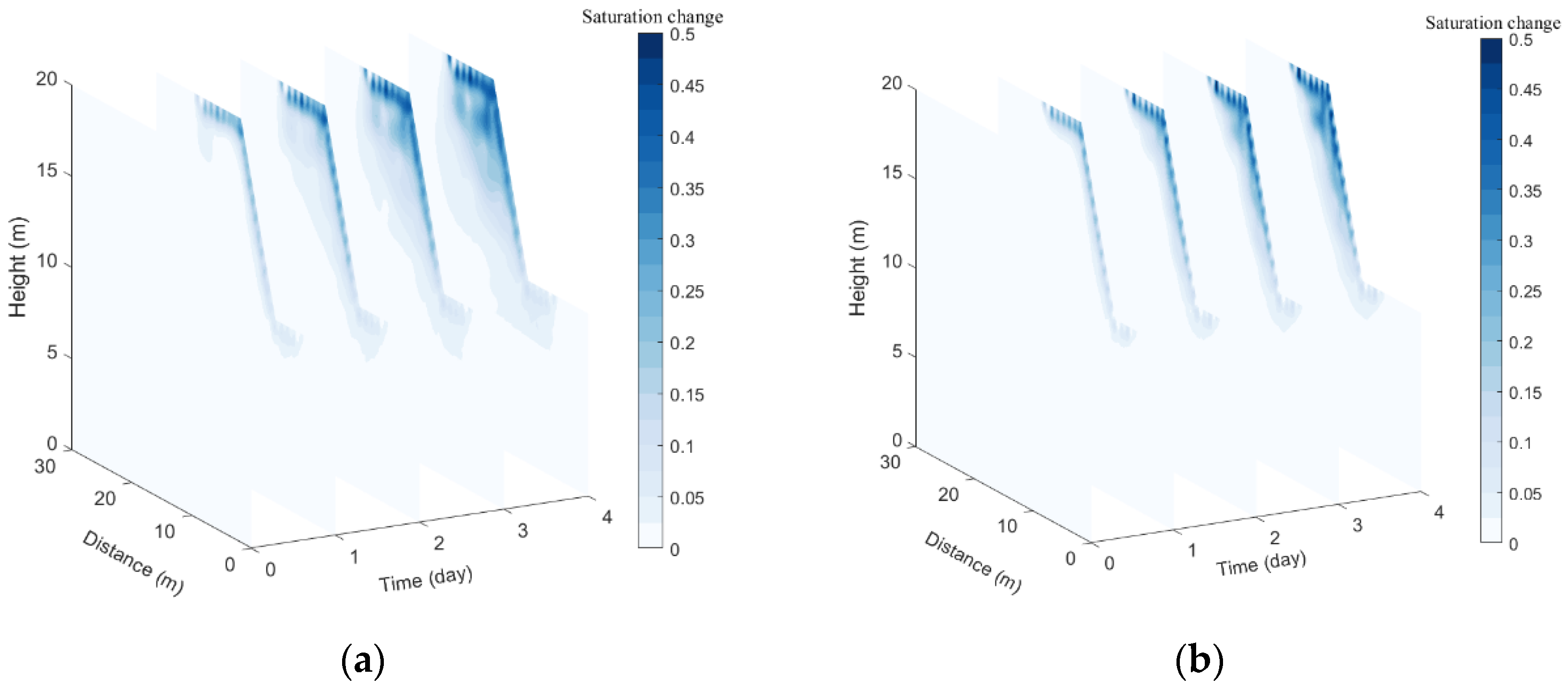
Figure 3a depicts the saturation distribution obtained under the aforementioned rainfall conditions. It should be noted that each cross section represents the saturation distribution at a separate time. In order to more clearly show the change in saturation distribution inside the landslide during the rainfall process, the saturation distribution at the initial moment is taken as the benchmark, and the saturation distribution at other moments is subtracted from it to obtain the change in saturation distribution at different moments, as shown in Figure 3b. According to Figure 3a,b, the slope body’s surface zone first experiences a rise in water content with the continuous infiltration of rainfall, and the zone with the increased water content then gradually extends to the lower zone. The matrix suction begins to decrease after the surface zone’s water content rises. The infiltration capacity of soil also decreases significantly, and the speed of water transport downward becomes slower and slower until it eventually tends to stabilize.

3.3. The Effect of the Arrays

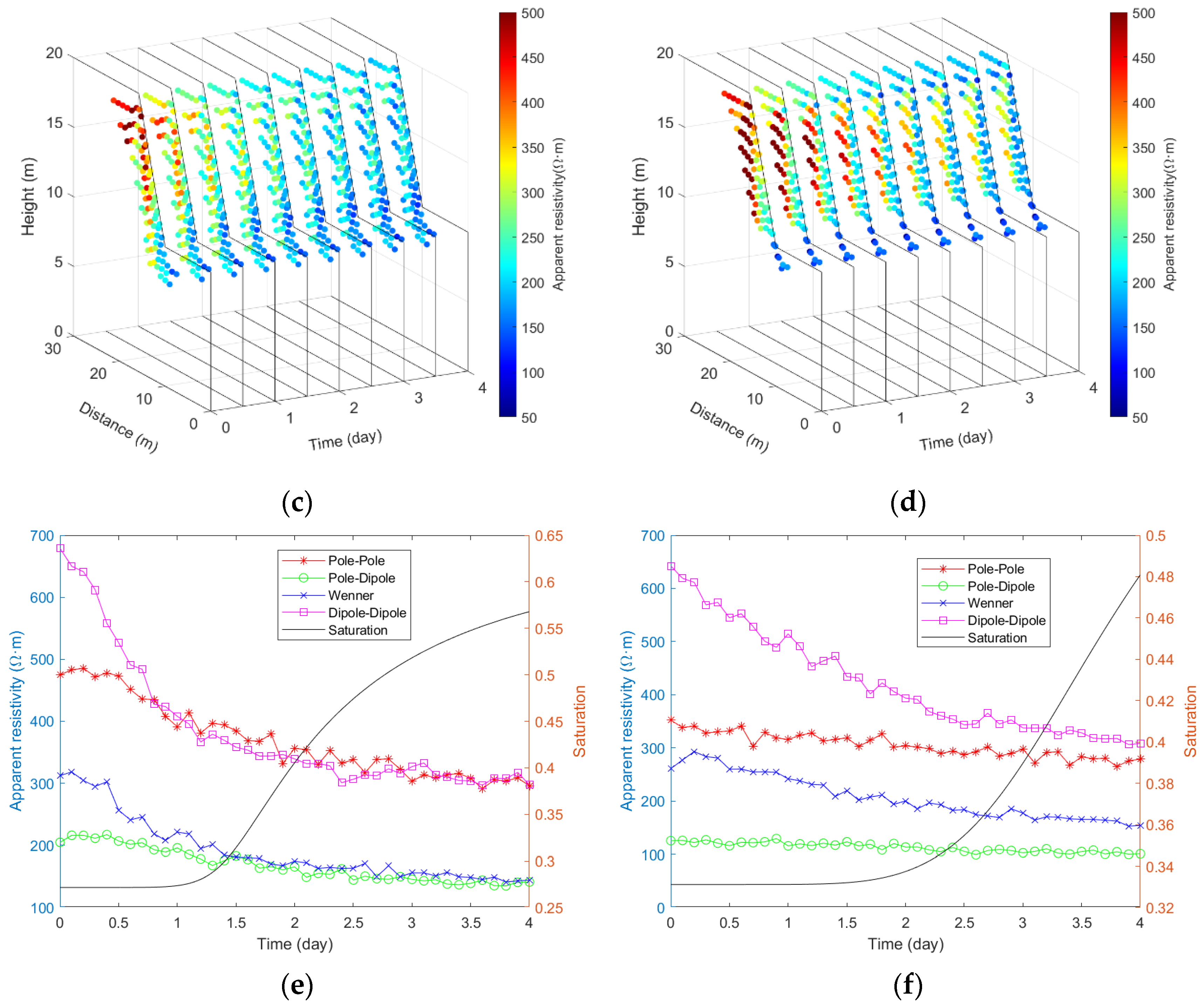
Different arrays must first be selected when using ERT. There are four types of arrays that are frequently used: Pole-Pole, Pole-Dipole, Wenner, and Dipole-Dipole [34,47]. Each type of array has unique properties. In experiments 1, 2, 3, and 4, the noise of the apparent resistivity responses and the uncertainty of WECC are adjusted to zero, and only the influence of the array is taken into account in order to compare and validate the detection effect of various arrays under rainfall conditions. The apparent resistivity responses obtained from forward modeling of various arrays during rainfall are shown in Figure 4, where subplots (a)–(d) show the apparent resistivity distributions from four arrays, Pole-Pole, Pole-Dipole, Wenner, and Dipole-Dipole, respectively, at different moments, and subplots (e) and (f) show the evolution of the apparent resistivity with saturation at two monitoring points, A and B, respectively.

Figure 4 shows that the apparent resistivity response recorded by each of the four arrays drops to varying degrees in response to the rise in saturation in the early stages of rainfall. As time goes on, the apparent resistivity drops less and tends to plateau, indicating the slowing down of the rate of change in water content in the landslide in the later period of rainfall. According to the apparent resistivity, which decreases in the order of Dipole-Dipole, Wenner, Pole-Pole, and Pole-Dipole, the Dipole-Dipole array is the most sensitive to saturation, followed by the Wenner array, and the Pole-Dipole array is the least sensitive.

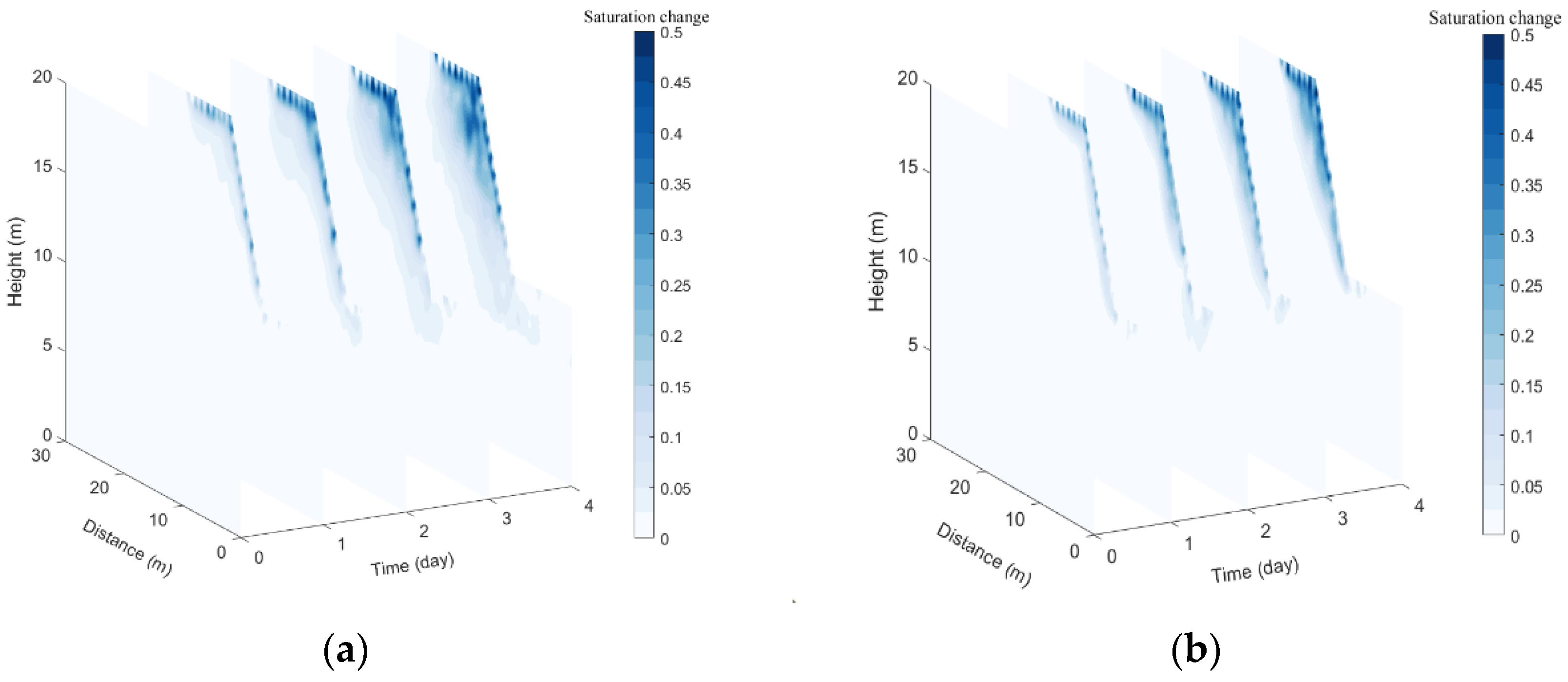
The inexact Gauss–Newton inversion based on multiple constraints is applied to the apparent resistivity response data obtained using these four arrays, and then the saturation distribution can be calculated using WECC. The variation in the saturation distribution of different arrays at different moments by inversion with respect to the initial saturation distribution is shown in Figure 5. Finally, the saturation results of the inversion are imported into COMSOL to calculate the FOS at different moments, as shown in

Table 3. The FOS obtained by the proposed framework in the noiseless scenario of multiple arrays.

		Theoretical Values	Pole-Pole	Pole-Dipole	Wenner	Dipole-Dipole
Time (day)	0	1.519	1.500	1.270	1.516	1.500
	1	1.494	1.490	1.390	1.485	1.499
	2	1.480	1.475	1.400	1.474	1.488
	3	1.463	1.455	1.060	1.443	1.468
	4	1.444	1.425	1.340	1.424	1.456
RMSE		-	0.013	0.224	0.014	0.011
MAPE		-	0.720	12.681	0.778	0.664

.

As shown by comparing the results of Figure 5 with Figure 3b, the inversion results of the four arrays can accurately reflect the water infiltration process in the ERT detection area, but the individual arrays have different features. Because the potential near the point source is singular, the saturation of the inversions of the four arrays increases there much more than it does elsewhere. The Pole-Pole array’s inversions reveal artifacts in the deeper regions, and these artifacts worsen as the infiltration process progresses. Combining the two indicators of RMSE and MAPE and the FOS calculated by the four arrays in Table 3, it can be found that the accuracy of the FOS calculated by the inversion of the three arrays is Dipole-Dipole, Pole-Pole, Wenner, and Pole-Dipole in descending order. The Pole-Dipole array, which has the lowest sensitivity, has a very large difference between calculated and theoretical values, whereas the Dipole-Dipole, Pole-Pole, and Wenner arrays have very small differences. This shows that the Dipole-Dipole, Pole-Pole, and Wenner arrays can theoretically be used to track the evolution of the FOS of landslides under rainfall conditions.

3.4. The Effect of the Apparent Resistivity Response Noise

Affected by the environment and the precision of the acquisition equipment, the apparent resistivity response of the field acquisition must contain noise, which requires the array used for the acquisition to have a certain degree of anti-noise capability. In Experiments 5, 6, 7, and 8, we applied a 3% Gaussian noise to the synthetic data obtained from forward modeling using different arrays in Experiments 1, 2, 3, and 4. The apparent resistivity responses obtained with various arrays in the presence of noise are shown in Figure 6, where subplots (a)–(d) show the apparent resistivity distributions from four arrays, Pole-Pole, Pole-Dipole, Wenner, and Dipole-Dipole, respectively, at different moments, and subplots (e) and (f) show the evolution of the apparent resistivity with saturation at two monitoring points, A and B, respectively. It can be seen from Figure 6e,f that the apparent resistivity response of various arrays in the presence of noise essentially has the same characteristics as in the absence of noise. It remains that Dipole-Dipole has the strongest sensitivity to water content, followed by Wenner, and Pole-Pole and Pole-Dipole have the weakest. The decrease in apparent resistivity response of the Pole-Pole and Pole-Dipole arrays is likely to be masked by noise in the presence of noise, which is particularly severe at monitoring site B (see Figure 6f). This also reflects the fact that as detection depth grows, lower resolution results, as the detection performance of both arrays becomes progressively less noise-resistant.

The acquired noise-containing apparent resistivity response data are calculated using the inexact Gauss–Newton algorithm for inversion based on multiple constraints and WECC for water-electric conversion to obtain the spatiotemporal evolution of the observed saturation of these four arrays, as shown in Figure 7a–d. From Figure 7a–d, it can be found that the spatiotemporal response pattern of saturation of the four arrays with noise is basically the same as that without noise, but the artifacts of the Wenner array also appear in the inner region, and the Pole-Pole and Pole-Dipole arrays show more serious artifacts at the foot of the slope (at point f in Figure 2), which may have a greater impact on the stability of the landslide.

Table 4. The FOS obtained by the proposed framework in the 3% Gaussian noise scenario of multiple arrays.

		Theoretical Values	Pole-Pole	Pole-Dipole	Wenner	Dipole-Dipole
Time (day)	0	1.519	1.535	1.420	1.494	1.493
	1	1.494	1.395	1.120	1.456	1.480
	2	1.480	1.055	1.220	1.410	1.507
	3	1.463	1.415	1.273	1.405	1.484
	4	1.444	1.360	1.330	1.380	1.451
RMSE		-	0.200	0.230	0.053	0.021
MAPE		-	9.084	13.976	3.440	1.296

displays the FOS calculated in the noise-containing environment using various arrays. It can be shown that noise has some effect on the calculations of all four arrays, with the Pole-Pole and Pole-Dipole arrays experiencing the worst impact. As a result, it is already difficult to depict the changing trend of FOS during rainfall infiltration. The Wenner and Dipole-dipole arrays can still indicate the change in FOS during rainfall infiltration, although they are also somewhat influenced by the noise-containing environment. This indicates that these two arrays have some noise resistance, with the Dipole-Dipole array having the best anti-noise capability.

3.5. The Effect of WECC Uncertainty

Although Archie’s formula can effectively fit the relationship between resistivity and water content, this smooth-fitting model ignores the relationship’s uncertainty, so it is still necessary to verify the impact of this uncertainty on the calculated FOS. When comparing the results of Experiments 1 through 8, it can be seen that the Wenner array and Dipole-Dipole array perform substantially better than the Pole-Pole array and Pole-Dipole array. For this reason, only the Wenner array and Dipole-Dipole array were utilized in Experiments 9 and 10. The resistivity calculated using Archie’s formula was added with 3% Gaussian noise to simulate WECC uncertainty during the data preparation phase of these two experiments after obtaining the saturation distribution at various times via COMSOL calculations. Finally, forward modeling was carried out to determine the apparent resistivity responses, which are depicted in Figure 8a–d, where Subplots (a) and (b) show the apparent resistivity values of the Wenner array and Dipole-Dipole array at different moments, respectively, and subplots (c) and (d) show the apparent resistivity changes at the two monitoring points A and B, respectively.

From Figure 8a–d, it can be found that the apparent resistivity responses obtained from both arrays after increasing the uncertainty of WECC by 3% still decreased with the increase in saturation, and the decrease in the apparent resistivity response of the Dipole-Dipole array was significantly larger than that of the Wenner array, which is consistent with the results of experiments 3, 4, 7, and 8, indicating that the Dipole-Dipole array is more sensitive to saturation than the Wenner array.

The inexact Gauss–Newton method based on multiple constraints is utilized for the inversion of the apparent resistivity response in Figure 8, and the Archie formula is then used to determine the saturation’s spatial and temporal distribution. Figure 9 displays the results. Finally, the FOS was calculated by SRM using COMSOL software, and the results are shown in

Table 5. The FOS obtained by the proposed framework in the 3% WECC uncertainty noise scenario of multiple arrays.

		Theoretical Values	Wenner	Dipole-Dipole
Time (day)	0	1.519	1.505	1.495
	1	1.494	1.475	1.490
	2	1.480	1.460	1.485
	3	1.463	1.430	1.465
	4	1.444	1.405	1.455
RMSE		-	0.026	0.012
MAPE		-	1.677	0.627

. According to Figure 9a,b and Table 5, the saturation distributions calculated for both arrays with the 3% increase in uncertainty in WECC are essentially the same as the distributions when no noise is added, and the FOS values calculated for both are also less different from the theoretical FOS. The FOS calculated with the Dipole-Dipole array is closer to the theoretical FOS than the Wenner array based on the two indicators of RMSE and MAPE, showing that the FOS calculated with the Dipole-Dipole array is more applicable.

3.6. The Effects of Multiple Conditions

The effects of the apparent resistivity response noise and the uncertainty of the WECC were taken into account in Experiments 11 and 12, and the synthesized data are shown in Figure 10a–d, where subplots (a) and (b) show the apparent resistivity values of the Wenner array and Dipole-Dipole array at different moments, respectively, and subplots (c) and (d) show the apparent resistivity changes at the two monitoring points A and B, respectively. It can be found that the characteristics of the apparent resistivity response are basically consistent with those observed in multiple previous experiments. The spatiotemporal distribution of saturation and the FOS calculated using the proposed framework are shown in Figure 11a,b and

Table 6. The FOS obtained by the proposed framework under the combination of multiple conditions.

		Theoretical Values	Wenner	Dipole-Dipole
Time (day)	0	1.519	1.510	1.505
	1	1.494	1.485	1.490
	2	1.480	1.450	1.465
	3	1.463	1.420	1.445
	4	1.444	1.390	1.395
RMSE		-	0.034	0.025
MAPE		-	1.957	1.342

, respectively. It can be found that although the FOS in the complex environment where the two scenarios work together is less accurate than the previous experimental results, it can also reflect the decreasing trend in the FOS of the landslide during the rainfall process, and the Dipole-Dipole array is still more adequate than the Wenner array.

4. Discussion

With the application of ERT, information on the spatial and temporal distribution of water content inside a landslide can be gathered in a non-invasive manner and on a broad scale. At the same time, the coverage of the ERT is larger than point-based sensor monitoring. However, as ERT measured resistivity values cannot be directly related to physical and mechanical material properties, they cannot be used to determine the landslide’s current stability state. In this paper, we attempted to use the technical route of inversion of ERT observation data→conversion of resistivity to water content data using WECC→FEM-based SRM to quantitatively calculate the evolution of FOS of landslides under rainfall conditions, and we performed several experiments with synthetic data to validate the performance and reliability of the proposed framework.

The experiments presented in this study show that, under theoretical conditions, the apparent resistivity responses obtained by utilizing the four ERT arrays show a quick and then steady reduction with continuous rainfall infiltration. The inexact Gauss–Newton algorithm based on multiple constraints was adopted for inversion in the proposed framework, and the spatiotemporal response of the inverted saturation may generally mirror the spatiotemporal evolution of true saturation. The FOS determined by the proposed framework could adequately reflect the evolution of the overall safety status of the landslide during rainfall, proving the performance and dependability of the proposed framework. However, the results of the conducted experiments show that the proposed framework has some influence on the accuracy and reliability of computation outcomes in complicated situations such as multiple arrays, apparent resistivity noise, and WECC uncertainty.

According to the results of Experiments 1–4, the apparent resistivity responses obtained from all four arrays showed a decreasing trend with continuous rainfall infiltration, and the decreasing magnitudes were, in descending order, Dipole-Dipole, Wenner, Pole-Pole, and Pole-Dipole. This means that the Dipole-Dipole array is the most sensitive to the change in saturation, followed by the Wenner array, then the Pole-Pole array, while the Pole-Dipole array was the least sensitive. This feature was also reflected in the subsequent experiments. This characteristic results from the fact that the resolution of each array varies, with the Dipole-Dipole array having the highest resolution among these four arrays. According to the computed results of saturation evolution and FOS derived by inversion, the Dipole-Dipole array has the best applicability, the Wenner and Pole-Pole arrays have the second-best applicability, and the Pole-Dipole array has the poorest applicability.

According to Experiments 5–8, the Dipole-Dipole array has the best anti-noise capability against apparent resistivity noise, while the Pole-Dipole array has the poorest. Combined with the analysis of the apparent resistivity response of the different arrays, the Dipole-Dipole array had the largest apparent resistivity decrease and the strongest sensitivity, and the presence of noise had little effect on this decreasing trend, whereas the Pole-Dipole array had the smallest decrease and the weakest sensitivity, and the presence of noise could easily drown out the apparent resistivity decrease.

Experiments 9 and 10 showed that when the Gaussian noise of WECC was increased by 3%, the FOS calculated by the proposed framework remained close to the theoretical value. Additionally, since the Dipole-Dipole array was most sensitive to saturation, the calculated FOS was also the closest to the theoretical value. These two experiments demonstrate the effectiveness of the proposed framework in considering the WECC uncertainty.

When the apparent resistivity response noise and the uncertainty of WECC were considered in Experiments 11 and 12, the FOS calculated by the method proposed in this paper remained relatively close to the theoretical value, indicating that it is theoretically feasible to use the ERT technique to calculate the landslide FOS and then carry out the landslide safety evaluation using the method proposed in this paper. All experimental results demonstrate that the Dipole-Dipole array exceeded other arrays in terms of accuracy, sensitivity, and noise resistance, whereas the Pole-Dipole array was less effective in all instances and is not recommended.

This paper used synthetic data for forward modeling. On the one hand, we needed to compare the calculation results of the proposed framework in different scenarios, and on the other hand, we currently lack the conditions to carry out actual landslide tests. In the future, ERT equipment that can be used for long-term, automatic monitoring can be deployed on actual landslide sites, and the sampling frequency and array can be designed according to specific needs so as to obtain ERT measurement data in near real time. The time series data from ERT monitoring can use the proposed framework to evaluate the FOS evolution of landslides and combine it with point-based monitoring data for analysis and judgment, thereby improving the accuracy and reliability of early warnings. At the same time, in practical application, it also will be necessary to solve problems such as the complexity of the internal structure of the landslide, the spatial variability of geotechnical parameters, and temperature interference. These challenges require continued research work in the future.

The framework proposed in this paper established the relationship between ERT observation data and landslide FOS, and it can use indirect ERT observation data to evaluate the evolution of a landslide’s safety status during the rainfall process. However, it should be mentioned that the computational complexity of the framework suggested in this research is extremely formidable, which is why two-dimensional experimental examples were adopted rather than three-dimensional experimental cases. The inversion process consumes a significant amount of computing time, and further research is required to increase computing speed and decrease computing time.

5. Conclusions

In this paper, a framework for calculating the FOS of landslides during rainfall using apparent resistivity response data from ERT monitoring was proposed. However, ERT data cannot be used directly for stability evaluation in landslide monitoring. The proposed framework first utilizes the inexact Gauss–Newton method inversion based on multiple constraints to acquire the resistivity distribution, then WECC to obtain the spatial and temporal distribution of saturation, and finally FEM-based SRM to calculate FOS. To evaluate the accuracy and reliability of the proposed framework, 12 sets of experiments were developed and carried out using synthetic data from the theoretical numerical model, then discussed and analyzed, yielding the following conclusions.

The numerical simulation results show that ERT monitoring data can reflect the spatial and temporal evolution of water content inside the landslide during rainfall, which can then be integrated with the values for physical and mechanical material properties in order to perform a quantitative safety evaluation of the landslide.

The quantitative computational approach described in this paper for calculating the FOS evolution of landslides by analyzing the apparent resistivity response of landslides during rainfall is reasonable and feasible.

The Dipole-Dipole array outperformed other ERT arrays (Wenner, Pole-Pole and Pole-Dipole) in terms of accuracy, sensitivity, and noise immunity. The Pole-Dipole array was least successful in all respects and is not recommended.

The noise of apparent resistivity response and the uncertainty of WECC had effects on the proposed framework’s calculation results. In practice, it is important not only to denoise the observation data but also to perform repeated calculations for the uncertainty of the relationship between the resistivity and the saturation, in order to increase the reliability of the calculation results.

Due to the need to validate the performance and reliability of the proposed method as well as the limitations of experimental conditions, in this study, synthetic data from the theoretical model were used. Subsequent studies are needed to obtain actual observation data from actual landslides to put the proposed theoretical framework into practical use. In the future, the work on actual landslides will still need to solve the problems of complex internal structure, spatial variation of geotechnical parameters, temperature interference, etc.

References

- Bai, D.; Tang, J.; Lu, G.; Zhu, Z.; Liu, T.; Fang, J. The design and application of landslide monitoring and early warning system based on microservice architecture. Geomat. Nat. Hazards Risk 2020, 11, 928–948. [Google Scholar] [CrossRef]
- Xia, C.; Lu, G.; Bai, D.; Zhu, Z.; Luo, S.; Zhang, G. Sensitivity Analyses of the Seepage and Stability of Layered Rock Slope Based on the Anisotropy of Hydraulic Conductivity: A Case Study in the Pulang Region of Southwestern China. Water 2020, 12, 2314. [Google Scholar] [CrossRef]
- Bai, D.; Lu, G.; Zhu, Z.; Zhu, X.; Tao, C.; Fang, J. A Hybrid Early Warning Method for the Landslide Acceleration Process Based on Automated Monitoring Data. Appl. Sci. 2022, 12, 6478. [Google Scholar] [CrossRef]
- Liu, Q.; Lu, G.; Dong, J. Prediction of landslide displacement with step-like curve using variational mode decomposition and periodic neural network. Bull. Eng. Geol. Environ. 2021, 80, 3783–3799. [Google Scholar] [CrossRef]
- Lee, K.; Suk, J.; Kim, H.; Jeong, S. Modeling of rainfall-induced landslides using a full-scale flume test. Landslides 2021, 18, 1153–1162. [Google Scholar] [CrossRef]
- Sheikh, R.; Nakata, Y.; Shitano, M.; Kaneko, M. Rainfall-induced unstable slope monitoring and early warning through tilt sensors. Soils Found. 2021, 61, 1033–1053. [Google Scholar] [CrossRef]
- Ahmed, F.S.; Bryson, L.S.; Crawford, M.M. Prediction of seasonal variation of in-situ hydrologic behavior using an analytical transient infiltration model. Eng. Geol. 2021, 294, 106383. [Google Scholar] [CrossRef]
- Chen, X.; Li, D.; Tang, X.; Liu, Y. A three-dimensional large-deformation random finite-element study of landslide runout considering spatially varying soil. Landslides 2021, 18, 3149–3162. [Google Scholar] [CrossRef]
- Tufano, R.; Formetta, G.; Calcaterra, D.; De Vita, P. Hydrological control of soil thickness spatial variability on the initiation of rainfall-induced shallow landslides using a three-dimensional model. Landslides 2021, 18, 3367–3380. [Google Scholar] [CrossRef]
- Gong, W.; Zhao, C.; Juang, C.H.; Zhang, Y.; Tang, H.; Lu, Y. Coupled characterization of stratigraphic and geo-properties uncertainties–A conditional random field approach. Eng. Geol. 2021, 294, 106348. [Google Scholar] [CrossRef]
- Archie, G.E. The Electrical Resistivity Log as an Aid in Determining Some Reservoir Characteristics. Trans. AIME 1942, 146, 54–62. [Google Scholar] [CrossRef]
- Mao, Y.; Romero, E.; Gens, A. Exploring ice content on partially saturated frozen soils using dielectric permittivity and bulk electrical conductivity measurements. E3S Web Conf. 2016, 9, 07005. [Google Scholar] [CrossRef]
- Merritt, A.J.; Chambers, J.E.; Wilkinson, P.B.; West, L.J.; Murphy, W.; Gunn, D.; Uhlemann, S. Measurement and modelling of moisture—electrical resistivity relationship of fine-grained unsaturated soils and electrical anisotropy. J. Appl. Geophys. 2016, 124, 155–165. [Google Scholar] [CrossRef] [Green Version]
- Cho, Y.; Dolan, S.S.; Saxena, N.; Das, V. Estimation of Water Saturation in Shale Formation Using In Situ Multifrequency Dielectric Permittivity. Geofluids 2022, 2022, e9491979. [Google Scholar] [CrossRef]
- Moreno, Z. Fine-scale heterogeneous structure impact on the scale-dependency of the effective hydro-electrical relations of unsaturated soils. Adv. Water Resour. 2022, 162, 104156. [Google Scholar] [CrossRef]
- Falae, P.O.; Kanungo, D.P.; Chauhan, P.K.S.; Dash, R.K. Electrical resistivity tomography (ERT) based subsurface characterisation of Pakhi Landslide, Garhwal Himalayas, India. Environ. Earth Sci. 2019, 78, 430. [Google Scholar] [CrossRef]
- Friedel, S.; Thielen, A.; Springman, S.M. Investigation of a slope endangered by rainfall-induced landslides using 3D resistivity tomography and geotechnical testing. J. Appl. Geophys. 2006, 60, 100–114. [Google Scholar] [CrossRef]
- Beff, L.; Günther, T.; Vandoorne, B.; Couvreur, V.; Javaux, M. Three-dimensional monitoring of soil water content in a maize field using Electrical Resistivity Tomography. Hydrol. Earth Syst. Sci. 2013, 17, 595–609. [Google Scholar] [CrossRef] [Green Version]
- Whiteley, J.S.; Chambers, J.E.; Uhlemann, S.; Wilkinson, P.B.; Kendall, J.M. Geophysical Monitoring of Moisture-Induced Landslides: A Review. Rev. Geophys. 2019, 57, 106–145. [Google Scholar] [CrossRef] [Green Version]
- Lapenna, V.; Perrone, A. Time-Lapse Electrical Resistivity Tomography (TL-ERT) for Landslide Monitoring: Recent Advances and Future Directions. Appl. Sci. 2022, 12, 1425. [Google Scholar] [CrossRef]
- Perrone, A.; Lapenna, V.; Piscitelli, S. Electrical resistivity tomography technique for landslide investigation: A review. Earth-Sci. Rev. 2014, 135, 65–82. [Google Scholar] [CrossRef]
- Drahor, M.G.; Göktürkler, G.; Berge, M.A.; Kurtulmuş, T. Application of electrical resistivity tomography technique for investigation of landslides: A case from Turkey. Environ. Geol. 2006, 50, 147–155. [Google Scholar] [CrossRef]
- Podolszki, L.; Kosović, I.; Novosel, T.; Kurečić, T. Multi-Level Sensing Technologies in Landslide Research—Hrvatska Kostajnica Case Study, Croatia. Sensors 2022, 22, 177. [Google Scholar] [CrossRef]
- Geng, J.; Sun, Q.; Zhang, Y.; Yan, C.; Zhang, W. Electric-field response based experimental investigation of unsaturated soil slope seepage. J. Appl. Geophys. 2017, 138, 154–160. [Google Scholar] [CrossRef]
- Liu, Y.; Lü, C.; Sun, Q. Geoelectric Field Response to Seepage in Sand and Clay Formations. J. Hydrol. Eng. 2019, 24, 04019037. [Google Scholar] [CrossRef]
- Hojat, A.; Arosio, D.; Ivanov, V.I.; Longoni, L.; Papini, M.; Scaioni, M.; Tresoldi, G.; Zanzi, L. Geoelectrical characterization and monitoring of slopes on a rainfall-triggered landslide simulator. J. Appl. Geophys. 2019, 170, 103844. [Google Scholar] [CrossRef]
- Lyu, C.; Sun, Q.; Zhang, W. Real-Time Geoelectric Monitoring of Seepage into Sand and Clay Layer. Ground Water Monit. Remediat. 2019, 39, 80–88. [Google Scholar] [CrossRef]
- Zeng, R.Q.; Meng, X.M.; Zhang, F.Y.; Wang, S.Y.; Cui, Z.J.; Zhang, M.S.; Zhang, Y.; Chen, G. Characterizing hydrological processes on loess slopes using electrical resistivity tomography–A case study of the Heifangtai Terrace, Northwest China. J. Hydrol. 2016, 541, 742–753. [Google Scholar] [CrossRef]
- Uhlemann, S.; Chambers, J.; Wilkinson, P.; Maurer, H.; Merritt, A.; Meldrum, P.; Kuras, O.; Gunn, D.; Smith, A.; Dijkstra, T. Four-Dimensional Imaging of Moisture Dynamics during Landslide Reactivation: Imaging of Landslide Moisture Dynamics. J. Geophys. Res. Earth Surf. 2016, 122, 398–418. [Google Scholar] [CrossRef] [Green Version]
- Boyle, A.; Wilkinson, P.B.; Chambers, J.E.; Meldrum, P.I.; Uhlemann, S.; Adler, A. Jointly reconstructing ground motion and resistivity for ERT-based slope stability monitoring. Geophys. J. Int. 2017, 212, 1167–1182. [Google Scholar] [CrossRef]
- Denchik, N.; Gautier, S.; Dupuy, M.; Batiot-Guilhe, C.; Lopez, M.; Léonardi, V.; Geeraert, M.; Henry, G.; Neyens, D.; Coudray, P.; et al. In-situ geophysical and hydro-geochemical monitoring to infer landslide dynamics (Pégairolles-de-l’Escalette landslide, France). Eng. Geol. 2019, 254, 102–112. [Google Scholar] [CrossRef]
- Boyd, J.; Chambers, J.; Wilkinson, P.; Peppa, M.; Watlet, A.; Kirkham, M.; Jones, L.; Swift, R.; Meldrum, P.; Uhlemann, S.; et al. A linked geomorphological and geophysical modelling methodology applied to an active landslide. Landslides 2021, 18, 2689–2704. [Google Scholar] [CrossRef]
- Manoli, G.; Rossi, M.; Pasetto, D.; Deiana, R.; Ferraris, S.; Cassiani, G.; Putti, M. An iterative particle filter approach for coupled hydro-geophysical inversion of a controlled infiltration experiment. J. Comput. Phys. 2015, 283, 37–51. [Google Scholar] [CrossRef]
- Carey, A.M.; Paige, G.B.; Carr, B.J.; Dogan, M. Forward modeling to investigate inversion artifacts resulting from time-lapse electrical resistivity tomography during rainfall simulations. J. Appl. Geophys. 2017, 145, 39–49. [Google Scholar] [CrossRef]
- Crawford, M.M.; Bryson, L.S. Assessment of active landslides using field electrical measurements. Eng. Geol. 2018, 233, 146–159. [Google Scholar] [CrossRef]
- Crawford, M.M.; Bryson, L.S.; Woolery, E.W.; Wang, Z. Using 2-D electrical resistivity imaging for joint geophysical and geotechnical characterization of shallow landslides. J. Appl. Geophys. 2018, 157, 37–46. [Google Scholar] [CrossRef]
- Crawford, M.M.; Bryson, L.S.; Woolery, E.W.; Wang, Z. Long-term landslide monitoring using soil-water relationships and electrical data to estimate suction stress. Eng. Geol. 2019, 251, 146–157. [Google Scholar] [CrossRef]
- Pidlisecky, A.; Haber, E.; Knight, R. RESINVM3D: A 3D resistivity inversion package. Geophysics 2007, 72, H1–H10. [Google Scholar] [CrossRef]
- Li, C.-W.; Xiong, B.; Qiang, J.-K.; Lü, Y.-Z. Multiple linear system techniques for 3D finite element method modeling of direct current resistivity. J. Cent. South Univ. 2012, 19, 424–432. [Google Scholar] [CrossRef]
- Liu, W.; Wang, H.; Xi, Z.; Zhang, R.; Huang, X. Physics-Driven Deep Learning Inversion with Application to Magnetotelluric. Remote Sens. 2022, 14, 3218. [Google Scholar] [CrossRef]
- Vu, M.T.; Jardani, A. Convolutional neural networks with SegNet architecture applied to three-dimensional tomography of subsurface electrical resistivity: CNN-3D-ERT. Geophys. J. Int. 2021, 225, 1319–1331. [Google Scholar] [CrossRef]
- Tikhonov, A.N.; Goncharsky, A.; Stepanov, V.V.; Yagola, A.G. Numerical Methods for the Solution of Ill-Posed Problems; Springer Science & Business Media: Berlin/Heidelberg, Germany, 1995; ISBN 978-0-7923-3583-2. [Google Scholar]
- Engl, H.W.; Grever, W. Using the L--curve for determining optimal regularization parameters. Numer. Math. 1994, 69, 25–31. [Google Scholar] [CrossRef]
- Van Genuchten, M.T. A Closed-form Equation for Predicting the Hydraulic Conductivity of Unsaturated Soils. Soil Sci. Soc. Am. J. 1980, 44, 892–898. [Google Scholar] [CrossRef] [Green Version]
- Lv, Y. Study on Stability of Unsaturated Soil Slope under Rainfall Condition Based on Xingye District. Master’s Thesis, Guilin University of Technology, Guilin, China, 2020. [Google Scholar]
- Qian, W.; Li, J.; Shan, X. Application of synoptic-scale anomalous winds predicted by medium-range weather forecast models on the regional heavy rainfall in China in 2010. Sci. China Earth Sci. 2013, 56, 1059–1070. [Google Scholar] [CrossRef]
- Zakaria, M.T.; Muztaza, N.M.; Zabidi, H.; Salleh, A.N.; Mahmud, N.; Rosli, F.N. Integrated analysis of geophysical approaches for slope failure characterisation. Environ. Earth Sci. 2022, 81, 299. [Google Scholar] [CrossRef]
Figure 1.
The proposed framework for calculating the evolution of landslides’ safety factors during rainfall.
Figure 2.
Slope geometry and boundary conditions setup for the used model (unit: m).
Figure 3.
Saturation distribution and saturation variation from numerical simulation: (a) Saturation distribution; (b) Saturation variation.
Figure 4.
Apparent resistivity response of various arrays during rainfall: (a) Pole-Pole array; (b) Pole-Dipole array; (c) Wenner array; (d) Dipole-Dipole array. (e) The evolution of apparent resistivity and saturation at point A with time. (f) The evolution of apparent resistivity and saturation at point B with time.
Figure 5.
The spatial and temporal evolution of moisture obtained by inversion of various arrays without noise: (a) Pole-Pole array; (b) Pole-Dipole array; (c) Wenner array; (d) Dipole-Dipole array.
Figure 6.
Apparent resistivity response with 3% Gaussian noise of various arrays during rainfall: (a) Pole-Pole array; (b) Pole-Dipole array; (c) Wenner array; (d) Dipole-Dipole array. (e) The evolution of apparent resistivity and saturation at point A with time. (f) The evolution of apparent resistivity and saturation at point B with time.
Figure 7.
The spatial and temporal evolution of saturation obtained by inversion under the condition of 3% Gaussian noise of various arrays: (a) Pole-Pole array; (b) Pole-Dipole array; (c) Wenner array; (d) Dipole-Dipole array.
Figure 8.
Apparent resistivity response of WECC for Wenner and Dipole-Dipole arrays with 3% uncertainty. (a) Wenner array, (b) Dipole-Dipole array. (c) Apparent resistivity and saturation at point A with time. (d) Apparent resistivity and saturation at point B with time.
Figure 9.
The spatial and temporal evolution of saturation obtained by inversion with 3% uncertainty in WECC: (a) Wenner array; (b) Dipole-Dipole array.
Figure 10.
Apparent resistivity response of WECC for Wenner and Dipole-Dipole arrays with the combination of multiple conditions: (a) Wenner array; (b) Dipole-Dipole array. (c) Apparent resistivity and saturation at point A with time. (d) Apparent resistivity and saturation at point B with time.
Figure 11.
The spatial and temporal evolution of saturation obtained by inversion under the combination of multiple conditions: (a) Wenner array; (b) Dipole-Dipole array.